Eternal inflation and energy conditions in de Sitter spacetime

Abstract

Eternal inflation is shown to require violations of the Null Energy Condition (NEC) on superhorizon scales. With light scalar fields as the matter sources in a de Sitter background, there can be no classical or semiclassical violations of the NEC. However, quantum fluctuations of the energy-momentum tensor, described by an expectation value of four field operators, do lead to large-scale NEC violations. The backreaction of such quantum fluctuations on the inflating spacetime is generally deduced at a heuristic level and leads to the eternal inflation scenario. A rigorous treatment of the backreaction will necessarily include fluctuations of the metric, and several new effects are expected to come into play.

I Eternal inflation scenario

Inflation is based on the dynamics of a scalar field in an expanding universe. For example, as shown in Fig. 1, the homogeneous mode of a massive, non-interacting, scalar field, $\phi$, could be high up on the potential, $V(\phi)$, at some initial epoch. Assuming that the dynamics is dominated by the homogeneous mode, the large potential energy of the field would cause exponential expansion (inflation) as long as the rate at which the field rolls down the potential is slow. As the field rolls, the potential energy diminishes, and the Hubble expansion slows down.

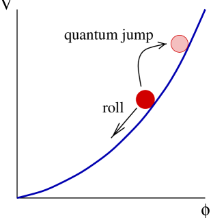
Figure 1: Illustration of the inflationary and eternal inflationary scenarios.

Eternal inflation modifies this picture of inflation by acknowledging that the field is really undergoing quantum dynamics. This means that there are uncertainties associated with the location of the field. Occasionally the field need not roll down the potential; instead it can jump up the potential. After this jump, the field is higher up, the potential energy is greater, and if the kinetic energy is not too large, the Hubble expansion speeds up. This is the basic idea of eternal inflation Ste83 ; Vil83 ; Lin86a ; Lin86b ; Lin86c ; Lin87 ; GonLin87 ; GonLinMuk87 .

Developing the scenario further, we can expect the same sort of behavior from scalar field modes that are smooth on large scales but not completely homogeneous. Then there will be regions in which the field will jump up. Such regions will form bubbles of faster inflation in a background of slower inflation. Indeed, even as the field in some regions rolls down to the minimum value of the potential, there will always be bubbling regions, and inflation will be eternal. The universe as we see it will only develop in regions that manage to roll down all the way and thermalize.

II Why bother with eternal inflation?

The eternal inflation scenario is attractive from a number of viewpoints. To the particle physicist or string theorist who is interested in cosmology, eternal inflation is simply a consequence of having a scalar field in a de Sitter background. If this simple combination results in eternal inflation, then it is very compelling and of fundamental importance. To the cosmologist, eternal inflation relieves certain concerns about the initial conditions that are essential for inflation Pir86 ; KunBra89 ; KunBra90 ; GolPir90 ; Gol91 ; VacTro98 ; TroVac99 ; Vac99 ; BerGor01 ; LueStaVac03 . No matter how the universe started out, once it undergoes even a bit of inflation, eternal inflation sets in. So the initial conditions become irrelevant Gut00 . To the general physicist, eternal inflation leads to a radically new picture of the universe, one which is bubbling forever, where new universes are constantly forming. This is the “multiverse” picture. Finally, to the observer, under certain circumstances and with certain assumptions, eternal inflation predicts a distribution of cosmological and other parameters that can be measured GarVil03 ; TegVil03 .

III The null energy condition

In a Friedman-Robertson-Walker universe, the equation governing the Hubble expansion, $H$, is:

$${\dot{H}}=-4\pi G(\rho+p)+\frac{k}{a^{2}}$$ (1)

where all the symbols have their usual meanings. In an inflating spacetime, the curvature term can be ignored and so we drop the last term. Then

$${\dot{H}}>0\Rightarrow\rho+p<0$$ (2)

We can write the latter condition in terms of the energy-momentum tensor $T_{\mu\nu}$ contracted with any null vector, $N^{\mu}$:

$$N^{\mu}N^{\nu}T_{\mu\nu}<0$$ (3)

In other words, the null energy condition (NEC) – $N^{\mu}N^{\nu}T_{\mu\nu}\geq 0$ – has to be violated if eternal inflation (${\dot{H}}>0$) is to happen BorVil97 .

The conclusion that one needs NEC violations to get eternal inflation can also be deduced from a spacetime diagram relevant to eternal inflation (see Fig. 2).

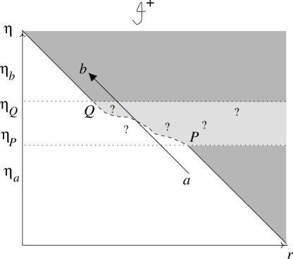
Figure 2: Spacetime diagram for eternal inflation. $\eta$ is the conformal time and $r$ is the comoving radial coordinate. Angular coordinates have been suppressed. At early times the solid line shows the radius of the minimal antitrapped sphere (MAS) in de Sitter space. The dashed portion of the line and question marks between the points $P$ and $Q$ represents the unknown position of the MAS during an upward jump. After the jump, the inverse horizon decreases but the spacetime is again de Sitter. So the MAS is again described by the solid line but the intercept on the $r=0$ axis is smaller (since $H^{-1}$ is smaller). A bundle of null geodesics traveling from point $a$ to $b$ goes from being converging at $a$ to diverging at $b$, in violation of the NEC.

IV Source of NEC violations?

We have seen that eternal inflation needs NEC violations. Now we try and determine if there exists a source for such violations. We will work within the context of a scalar field theory that is minimally coupled to gravity. The action is:

$$S=\int d^{4}x\sqrt{-g}\biggl{[}-\frac{1}{16\pi G}R+\frac{1}{2}(\partial_{\mu}\phi)^{2}-\frac{m^{2}}{2}\phi^{2}\biggr{]}$$ (4)

The scalar field, $\phi$, has energy-momentum tensor

$$T_{\mu\nu}=\nabla_{\mu}\phi\nabla_{\nu}\phi-\frac{1}{2}g_{\mu\nu}\left(\nabla^{\mu}\phi\nabla_{\mu}\phi-m^{2}\phi^{2}\right)\ .$$ (5)

IV.1 Classical field

If $N^{\mu}$ is any null vector ($g_{\mu\nu}N^{\mu}N^{\nu}=0$) then

$$N^{\mu}N^{\nu}T_{\mu\nu}=(N^{\mu}\partial_{\mu}\phi)^{2}\geq 0$$ (6)

and hence a classical scalar field cannot violate the NEC.

So, not surprisingly, to get eternal inflation, we must consider quantum field theory.

IV.2 Semiclassical gravity

In quantum field theory, the energy-momentum tensor becomes an operator. In semiclassical gravity, however, the metric is still classical. To relate the classical metric, to the quantum energy-momentum tensor, we use the semiclassical version of Einstein’s equation:

$$G_{\mu\nu}=8\pi G\langle s|T_{\mu\nu}|s\rangle$$ (7)

There are a few points about this equation that need to be explained. First, it is essential to specify the state, $|s\rangle$, of the quantum fields. In our case, we will take it to be the Bunch-Davies vacuum, as is normally done in inflationary calculations BraHil86 ; Albetal94 , and denote this state as $|0\rangle$ (It is well-known that with a non-vacuum choice of the state, the NEC can be violated EpsGlaJaf65 ; MorTho88 ; Kuo97 though the violations must still satisfy certain inequalities For93 ; ForRom95 .) Second, the expectation value of the energy-momentum tensor is going to be infinite. Hence we need to carry out a suitable renormalization procedure. For example, we will have to introduce a bare cosmological constant term that can be used to cancel out the infinite vacuum energy. The gravitational coupling constant will also be normalized. Once all these necessary renormalization procedures are carried out, we may write:

$$G_{\mu\nu}=8\pi G_{N}\langle 0|T_{\mu\nu}^{ren}|0\rangle$$ (8)

So the NEC is

$$N^{\mu}N^{\nu}\langle 0|T_{\mu\nu}^{ren}|0\rangle\geq 0$$ (9)

and we would like to check if this condition is violated.

The left-hand side of Eq. (8) is a tensor, hence the right-hand side had better be a second rank tensor too. Since the only tensor available to us in de Sitter spacetime is the metric, we immediately have:

$$\langle 0|T_{\mu\nu}^{ren}|0\rangle=Ag_{\mu\nu}$$ (10)

where $A$ is a constant. But then:

$$N^{\mu}N^{\nu}\langle 0|T_{\mu\nu}^{ren}|0\rangle=Ag_{\mu\nu}N^{\mu}N^{\nu}=0$$ (11)

and the NEC is not violated by a scalar field in de Sitter spacetime within the realm of semiclassical gravity.

IV.3 Fluctuations of the energy momentum tensor

Fluctuations of the renormalized energy-momentum tensor may show NEC violations even though the expectation value does not. Indeed, Eq. (11) shows that the expectation value of $N^{\mu}N^{\nu}T_{\mu\nu}^{ren}$ vanishes and hence any fluctuations in it will violate the NEC. To calculate the magnitude of the fluctuations, we need to consider:

$$\langle 0|N^{\mu}N^{\nu}T_{\mu\nu}^{ren}(x)N^{\lambda}N^{\sigma}T_{\lambda\sigma}^{ren}(x)|0\rangle$$

However, since the operators are evaluated at the same spacetime point, the fluctuations will be infinite.

This infinity is not a crisis since, after all, we are interested in NEC violations not at a single spacetime point but in an entire spacetime region. Hence we should consider fluctuations of a “smeared” operator, which we can define as:

$$T_{W}\equiv\int d^{4}y\sqrt{-g}\,W(y;x)N^{\mu}N^{\nu}T_{\mu\nu}^{ren}(y)$$ (12)

where $W(y;x)$ is a window function of our choosing, centered at $x$. Note that the smearing is both in space and time.

The NEC is violated if

$$\sigma^{2}\equiv\langle T_{W}^{2}\rangle-\langle T_{W}\rangle^{2}~{}>~{}\langle T_{W}\rangle^{2}\equiv\mu^{2}$$ (13)

Even without doing any calculation, we can see that NEC violating fluctuations must occur. From Eq. (11) we know that $\langle T_{W}\rangle=0$. The smearing in Eq. (12) ensures that the operators in $\langle T_{W}^{2}\rangle$ are multiplied at distinct spacetime points. The spacetime smearing ensures that $\langle T_{W}^{2}\rangle$ is finite. (To see this explicitly one needs to consider the integrals in more detail.) Also, we can expect $\langle T_{W}^{2}\rangle$ to be non-zero because there are no symmetries that force it to vanish. In fact, since the operator $T_{W}$ is non-trivial, even if $\langle T_{W}^{2}\rangle$ were to vanish for some choice of window function, expectation values of yet higher powers of $T_{W}$, e.g. $\langle T_{W}^{n}\rangle$ for $n>2$, could be considered. A non-vanishing result for any $n$ would indicate NEC violating fluctuations.

In the case when the smearing scales are chosen to be given by the horizon size $H^{-1}$, there is only one dimensionful quantity in the problem and dimensional arguments can be used. Hence, in this case,

$$\langle T_{W}^{2}\rangle=\alpha H^{8}$$ (14)

where $\alpha\neq 0$ is a finite number. This result is already interesting. Since the expectation of $T_{W}$ vanishes, it says that there are both negative and positive fluctuations in $T_{W}$. Assuming that either sign is equally likely, this implies that the NEC is violated with 50% probability. The actual magnitude of the NEC violating fluctuation will depend on the parameter $\alpha$, which will also depend on the smearing function. On spatial and temporal scales given by the horizon, the magnitude of NEC violation is $\sqrt{\alpha}H^{4}$.

A few new issues arise when we try to do better than the dimensional estimate. First, for convenience, we choose the window function to be Gaussian in conformal time and space.

$$W\left(\eta,{\mathbf{r}}\right)=\frac{1}{\sqrt{-g}}\frac{a_{0}^{4}}{R^{3}\tau}W_{\eta}\left(\frac{\left|\eta-\eta_{0}\right|}{a_{0}^{-1}\tau}\right)W_{r}\left(\frac{\left|{\mathbf{r}}-{\mathbf{r}}_{0}\right|}{a_{0}^{-1}R}\right)$$ (15)

Here

$$a_{0}\equiv a\left(\eta_{0}\right),\quad\tau\equiv H^{-1}\tanh(HT)$$ (16)

and we have introduced the reference point $(\eta_{0},{\mathbf{r}}_{0})$ with $\eta_{0}\neq 0$, since $\eta=0$ is a singular point of the conformal coordinate system. (In our coordinates $\sqrt{-g}=\left(H\eta\right)^{-4}=a^{4}$.) The normalization of the window and of the null vector

$$N^{\mu}=a_{0}\left(H\eta\right)^{2}\left[1,{\mathbf{n}}\right].$$ (17)

is chosen to make the final result independent of $\eta_{0}$. The time-dependent normalization of the null vector $N^{\mu}$ is such that $N^{\mu}$ is affinely parametrized. For simplicity, the three vector ${\mathbf{n}}$ will be chosen to be the unit radial vector.

The parameter $\tau$ is defined so that averaging in conformal time $\eta$ with the window $a_{0}\tau^{-1}W_{\eta}\left(a_{0}\tau^{-1}|\eta-\eta_{0}|\right)$ corresponds to a window with proper time duration $T$ where the relation between conformal time, $\eta$, and proper time, $t$, is:

$$\eta=-H^{-1}e^{-Ht}=-\left(Ha\left(t\right)\right)^{-1}$$ (18)

Note that $H\tau<1$ always holds. Likewise, the spatial window in Eq. (15) is such that in the neighborhood of $\eta=\eta_{0}$ the proper length corresponding to the spatial averaging is $R$.

In addition, we generalize the calculation to be more applicable to inflationary cosmology where the de Sitter background changes due to a slowly rolling scalar field. Then the scalar field is given by:

$$\phi=\phi_{0}+\delta\phi$$ (19)

where $\phi_{0}$ denotes the coherent state representing the rolling field and $\delta\phi$ denotes quantum fluctuations. Since the field value is now changing with time, $\mu\equiv\langle T_{W}\rangle\neq 0$ and is given by the kinetic energy in $\phi_{0}$:

$$\mu=\frac{1}{2}{\dot{\phi}}_{0}^{2}\ .$$ (20)

The calculation of $\sigma^{2}$ is now straightforward albeit tedious, requiring clever estimation of certain integrals. The final result will be given only for $R=T=(\varepsilon H)^{-1}$.

$$\sigma^{2}\sim\frac{H^{4}\dot{\phi}_{0}^{2}\max\left(c_{1}^{2}\varepsilon^{2},c_{1}^{\prime 2}\varepsilon^{4}\right)}{\left(2\pi\right)^{2}}+\frac{c_{2}^{2}H^{8}\varepsilon^{8}}{\left(2\pi\right)^{4}}$$ (21)

where $c_{1}$, $c_{1}^{\prime}$ and $c_{2}$ are constants. We have evaluated these constants numerically for the Gaussian window function and find them to be of order unity. The last term in Eq. (21) is new. It arises due to the expectation value of four creation and annihilation operators ($\langle aaa^{\dagger}a^{\dagger}\rangle$) and cannot be derived by simply considering root-mean-square fluctuations of the scalar field $\phi$. We can also compare the magnitude of the fluctuations to the square of the mean, as needed in Eq. (13):

$$\frac{\sigma^{2}}{\mu^{2}}\sim\frac{H^{4}\max\left(c_{1}^{2}\varepsilon^{2},c_{1}^{{}^{\prime}2}\varepsilon^{4}\right)}{\left(2\pi\dot{\phi}_{0}\right)^{2}}+\frac{c_{2}^{2}H^{8}\varepsilon^{8}}{\left(2\pi\dot{\phi}_{0}\right)^{4}}.$$ (22)

In the special case of an exactly de Sitter background (${\dot{\phi}}=0$), Eq. (21) gives:

$$\sigma^{2}\sim\frac{c_{2}^{2}H^{8}\varepsilon^{8}}{\left(2\pi\right)^{4}}$$ (23)

Since $\mu=0$ in this case, the very fact that $\sigma$ is non-vanishing implies that the NEC is violated.

It is fair to say that the detailed evaluation of $\sigma^{2}$ is not very crucial for us since here are only interested in knowing whether NEC violations exist. This was evident from Eq. (14) itself. Yet the detailed calculation is relevant when asking more quantitative questions. (What is the typical magnitude of an upward jump that is coherent on some given scale?) One subtlety in the detailed evaluation is that it is easier to do the calculation when the window function is chosen to be a Gaussian in conformal time, but much harder if it is Gaussian in proper time.

V Backreaction

Recall that our derivation in Sec. III for the necessity of NEC violations in eternal inflation was based on the classical Einstein equations. The derivation could also be extended using the semiclassical equations provided we think of $\rho$ and $p$ in Sec. III as being expectation values. However, what we have shown above is that NEC violations only occur in the fluctuations of the energy-momentum tensor in de Sitter spacetime. Such fluctuations do not couple to the metric by the classical or semiclassical Einstein equations. Then, what equations should we use to couple the metric and the energy-momentum quantum operator? Is there a smeared version of the Einstein or other equation? In other words, we need some prescription to determine the backreaction of the quantum fluctuations on the metric.

There are potentially two new effects that can arise when calculating the backreaction. First, we will need to let the metric fluctuate as well. Without such metric fluctuations, the semiclassical Einstein equations will hold and they imply that the Hubble expansion rate cannot grow as required in eternal inflation. Once the metric is allowed to fluctuate, there will be interactions with the scalar field fluctuations that will affect the NEC violating rate. (This is similar to gravitational corrections occurring in instanton amplitudes.) There will also be independent quantum fluctuations of the metric. For example, it is conceivable that even if one were to take a de Sitter background without any scalar field, the metric would fluctuate, and there would be regions that would expand slightly faster and others slightly slower. If so, one could presumably argue for an eternally inflating multiverse even without a scalar field. This would be quite interesting. The second new effect is that the fluctuation amplitude falls off with length scale. So if there is an upward jump in some local region, one might expect that the field outside this region will jump down to compensate. This effect might lead to interesting correlations of fluctuations. Another way to state this new effect is that whatever the scalar field energy-momentum tensor fluctuations may be, the semiclassical Einstein equations must still hold although in some average sense. Hence there can be no “overall” eternal inflation and local increases in the expansion rate must be accompanied by other local decreases in the expansion rate.

The current treatment of the backreaction in the literature assumes that if there is an NEC violating fluctuation, it simply resets the value of the scalar field on the potential and the metric itself does not participate in the fluctuation. After the fluctuation is over, we can revert to a classical description of the evolution with the reset value of the scalar field. Then eternal inflation follows as described in Sec. I.

VI Conclusions

The search for NEC violations in de Sitter spacetime was motivated by the classical Einstein equations. Within the realm of classical gravity and its semiclassical extension, no NEC violations were found. However, fluctuations of the energy-momentum tensor of a scalar field in de Sitter spacetime were found to violate the NEC. Hence one must look to the gravitational backreaction of energy-momentum tensor fluctuations to derive a convincing model of eternal inflation. In addition, one must also consider the quantum fluctuations of the metric itself.

In the literature, backreaction calculations have been attempted that fall into two categories. First is the backreaction of classical fluctuations BriHar64 ; Isa68 ; HuxPazZha93 ; MukFelBra92 . In these calculations, the classical Einstein equations always hold but corrections to a background metric (e.g. inflationary background) are evaluated in a perturbative manner. We have already seen that classical physics cannot give the required NEC violation and hence this approach cannot help with eternal inflation. The second category of backreaction calculations TsaWoo96 ; TsaWoo97 (summarized in Woo01 ) considers the effects of quantum fluctuations on the spacetime, and seems to be more suited to addressing eternal inflation. Presently the pioneers of this approach find that the metric fluctuations themselves – in a de Sitter spacetime with only a cosmological constant and without any scalar field – have a very strong effect on the de Sitter background and can switch off the inflation or even lead to a period of deflation. They understand this result physically in terms of the mutual gravitational attraction of gravitons produced by the inflating background. With this physical picture, since these are quantum effects and hence probabilistic, there will be local fluctuations in the number of gravitons and hence in the local Hubble expansion rate. One would have thought that the result of the calculation should then lead to eternal inflation even in the absence of a scalar field!

The eternal inflation scenario is seductive for a variety of reasons. At the moment, however, it rests on heuristic arguments. More rigorous calculations are needed to make it quantitative and convincing.

- (1) A. Guth, T. Vachaspati and S. Winitzki, unpublished.
- (2) P.J. Steinhardt, in “The Very Early Universe”, eds. G.W. Gibbons, S.T.C. Siklos and S.W. Hawking, Cambridge University Press (1983).
- (3) A. Vilenkin, Phys. Rev. D27, 2848 (1983).
- (4) A.D. Linde, Phys. Lett. B175, 395 (1986).
- (5) A.D. Linde, Mod. Phys. Lett. 1A, 81 (1986).
- (6) A.D. Linde, in Proceedings of the Nobel Symposium on Elementary Particle Physics, Physica Scripta 34 (1986).
- (7) A.D. Linde, in 300 Years of Gravitation, eds. S. W. Hawking and W. Israel (Cambridge University Press, 1987).
- (8) A.S. Goncharov and A.D. Linde, Zh. Eksp. Teor. Fiz. 92, 1137 (1987).
- (9) A. S. Goncharov, A. D. Linde and V. F. Mukhanov, Int. J. Mod. Phys. A2, 561 (1987).
- (10) T. Piran, Phys. Lett. B181, 238 (1986).
- (11) J.H. Kung and R. Brandenberger, Phys. Rev. D40, 2532 (1989).
- (12) J.H. Kung and R. Brandenberger, Phys. Rev. D42, 1008 (1990).
- (13) D.S. Goldwirth and T. Piran, Phys. Rev. Lett. 64, 2852 (1990).
- (14) D.S. Goldwirth, Phys. Rev. D43, 3204 (1991).
- (15) T. Vachaspati and M. Trodden, Phys. Rev. D61, 023502 (1999).
- (16) M. Trodden and T. Vachaspati, Mod. Phys. Lett. A14, 1661-1665 (1999).
- (17) T. Vachaspati, in proceedings of COSMO-98, ed. D. O. Caldwell (American Institute of Physics, New York, 1999).
- (18) A. Berera and C. Gordon, Phys. Rev. D63, 063505 (2001).
- (19) A. Lue, G.D. Starkman and T. Vachaspati, astro-ph/ 0303268 (2003).
- (20) A. Guth, Phys. Rept. 333, 555-574 (2000).
- (21) J. Garriga and A. Vilenkin, Phys. Rev. D67, 043503 (2003).
- (22) M. Tegmark and A. Vilenkin, astro-ph/0304536 (2003).
- (23) A. Borde and A. Vilenkin, Phys. Rev. D56, 717 (1997).
- (24) H. Epstein, V. Glaser and A. Jaffe, Nuovo Cim. 36, 1016 (1965).
- (25) M.S. Morris and K.S. Thorne, Am. J. Phys. 56, 395 (1988).
- (26) B. L. Hu, J. P. Paz, and Y. Zhang, in The Origin of Structure in the Universe, ed. by E. Gunzig and P. Nardone (Kluwer, Dordrecht 1993).
- (27) L. P. Grishchuk and Yu. V. Sidorov, Phys. Rev. D42, 3413 (1990).
- (28) R. Brandenberger and C. Hill, Phys. Lett. B179, 30 (1986).
- (29) A. Albrecht, P. Ferreira, M. Joyce and T. Prokopec, Phys. Rev. D50, 4807 (1994).
- (30) L.H. Ford, Phys. Rev. D48, 776 (1993);
- (31) L.H. Ford and T. Roman, Phys. Rev. D51, 4277 (1995).
- (32) C.-I. Kuo, Nuovo Cim. 112B, 629 (1997).
- (33) A. Vilenkin and L.H. Ford, Phys. Rev. D26, 1231 (1982).
- (34) D. Brill and J. Hartle, Phys. Rev. 135, 1B 271 (1964).
- (35) R. Isaacson, Phys. Rev. 166, 1263 (1968); 1272 (1968).
- (36) B.L. Hu, J.P. Paz, and Y. Zhang, in The Origin of Structure in the Universe, ed. by E. Gunzig and P. Nardone (Kluwer, Dordrecht 1993).
- (37) V.F. Mukhanov, H.A. Feldman and R.H. Brandenberger, Phys. Rept. 215, 203 (1992).
- (38) N.C. Tsamis and R.P. Woodard, Nucl. Phys. B474, 235 (1996).
- (39) N.C. Tsamis and R.P. Woodard, Ann. Phys. 267, 145 (1998).
- (40) R.P. Woodard, talk presented at COSMO-01, Rovaniemi, Finland; astro-ph/0111462 (2001).