Long Period Variables in NGC 5128: I. Catalogue

The first variable star catalogue in a giant elliptical galaxy NGC 5128 (Centaurus A) is presented. Using multi-epoch observations with ISAAC at the VLT we have detected 1504 red variables in two halo fields covering $10.46$ arcmin square. For the variables with at least 10 good measurements, periods and amplitudes were determined using Fourier analysis and non-linear sine-curve fitting algorithms. The final catalogue contains 1146 long period variables with well established light curve parameters. Periods, amplitudes, $J_{\rm s}HK_{\rm s}$ photometry as well as individual $K_{\rm s}$-band magnitudes are provided for all the variables. The distribution of amplitudes ranges from 0.3 to a few magnitudes in the $K_{\rm s}$-band, with a median value around 0.7 mag. The amplitudes, mean magnitudes and periods indicate that the majority of variables belong to the class of long period variables with semiregular and Mira variables. Exhaustive simulations were performed in order to assess the completeness of our catalogue and the accuracy of the derived periods.

1 Introduction

In a stellar population older than few hundred Myr the near-IR light is dominated by red giants. Of these, first ascent giants are the brightest among the metal-poor stars older than 1-2 Gyr. In composite stellar populations, like those found in galaxies, the first ascent giants are mixed with asymptotic giant branch (AGB) stars. The red giants fainter than the tip of the first ascent giant branch are usually referred to as red giant branch (RGB) stars. In the following RGB is used to denote the first ascent giants, although it should be kept in mind that it is not possible to separate RGB and AGB stars that are fainter than the RGB tip.

In intermediate-age populations ($\sim 1-5$ Gyr old) numerous bright asymptotic giant branch (AGB) stars are located above the tip of the RGB. However, among old populations like Galactic globular clusters with ${\rm[Fe/H]}\ga-1.0$ dex and in the Galactic bulge, bright stars have also been detected above the tip of the RGB (Frogel & Elias frogel&elias88 (1988), Guarnieri et al. guarnieri+97 (1997)), implying the presence of bright AGB stars in metal-rich and old populations. Essentially all of the bright giants above the RGB tip in globular clusters seem to be long period variables (LPVs; Frogel & Elias frogel&elias88 (1988), Frogel & Whitelock frogel&whitelock98 (1998)). The frequency of LPVs in old metal-rich globular clusters of the MW and in the Bulge has been studied by Frogel & Whitelock (frogel&whitelock98 (1998)). Old populations of lower metallicity are known not to have AGB stars brighter than the RGB tip. The presence or absence of these bright giants located above the tip of the first ascent giant branch has important implications for the magnitude of the surface brightness fluctuations specifically in the near-IR (e.g. Mei et al. mei+01 (2001), Liu et al. liu+02 (2002)), a method used to determine distances to galaxies that are too distant to have their stellar content resolved, but that still present fluctuations due to the underlying light of giant stars (Tonry & Schneider tonry&schneider88 (1988)).

The properties of LPVs have been reviewed by Habing (habing96 (1996)). They are thermally pulsing asymptotic giant branch (TP-AGB) stars with main sequence masses between 1 and 6 M_⊙. They present variability with periods of 80 days or longer, and often the longest period variables show variable or multiple periods. Two main classes of LPVs are Mira variables (Miras) and semiregular variables (SRs). SRs usually have smaller amplitudes as well as shorter periods and more irregular light curves than Miras. SRs are sometimes subdivided into subclasses (SRa, SRb) depending on the regularity and multiplicity of their periods and shape of their light curves. The separation between Miras and SRs is not always clear (e.g. Kerschbaum & Hron kerschbaum&hron92 (1992, 1994)). The classical definition requires that Miras have $V$-band amplitudes larger than 2.5 mag and regular periods in the range of 80–1000 days (GCVS Kholopov gcvs (1985)). Mean $K$-band amplitudes of Miras are $\sim 0.6$ mag (e.g. Feast et al. feast+82 (1982), Wood et al. wood+83 (1983)).

In the gE NGC 5128 Soria et al. (soria+96 (1996)), based on $VI$ HST CMD, and Marleau et al. (marleau+00 (2000)), based on $JH$ NICMOS data, suggested a presence of up to 10% bright AGB stars belonging to an intermediate-age population. Harris et al. (harris+99 (1999, 2000)) on the contrary did not find bright AGB stars in their $VI$ CMDs of two halo fields in NGC 5128. However, $V$ and $I$ bands are not very sensitive indicators of these cool giants and thus some of them might have been confused with the RGB tip or foreground stars and few stellar blends or stars with larger photometric errors.

Our group has obtained VLT images with FORS1 and ISAAC in the halo of NGC 5128 in order to study the bright giants in the halo of the galaxy (Rejkuba et al. rejkuba+01 (2001)). We have observed two halo fields in the $V$ and $K_{\rm s}$-bands finding a large number of bright AGB stars, extending up to bolometric magnitude of –5. Field 1 coincides with the prominent north-eastern diffuse stellar shell (Malin et al. malin+83 (1983), Rejkuba et al. rejkuba+01 (2001)). Crossing it in diagonal there is a chain of young stars (Mould et al. mould+00 (2000), Fassett & Graham fg00 (2000), Rejkuba et al. rejkuba+02 (2002)). Field 2 is located away from the known stellar shells and dust bands, $\sim 9\arcmin$ south from the galactic nucleus. It coincides with the field observed with HST in $V$ and $I$-bands with WFPC2 by Soria et al. (soria+96 (1996)) and in $J$ and $H$-bands with NICMOS by Marleau et al. (marleau+00 (2000)). Part of the VLT ISAAC $K_{\rm s}$-band data analyzed here were already described in Rejkuba et al. (rejkuba+01 (2001)). Already with the first few epochs of $K_{\rm s}$-band imaging it was obvious that variable stars were present among the bright red giants. The preliminary results of the multi-epoch imaging in $K_{\rm s}$-band were presented by Rejkuba (rejkubaPhd (2002)).

We present here the full near-IR data-set containing multi-epoch $K_{\rm s}$-band imaging and single-epoch data in the $J_{\rm s}$- and $H$-bands obtained over the period of 3 years with ISAAC at the VLT. In this paper the data reduction, the photometry, and the catalogue of the variable stars are presented. In the following papers these data are used to investigate the variability characteristics of the population of stars found above the RGB tip, and to derive the distance to NGC 5128 using the Mira period-luminosity relation in the $K$-band. Multicolor information will further be used to investigate the chemical composition of these variables, and to put constraints to their ages. In the next section we briefly present the data and the reduction procedures. Section 3 contains the photometry. The technique used to detect the variable stars is described next. The light curves and periods of the long period variables are derived in Sect. 5. A detailed description of the completeness simulations is given only in the electronic version of the article where also the complete catalogue of all the variable stars can be found. Sect. 6 presents the main results of the our simulations, while the last section summarizes the results.

2 The data

2.1 The observations

We have obtained a total of 20 epochs of $K_{\rm s}$-band photometry in Field 1 and 24 epochs in Field 2 between April 1999 and July 2002. Most of our data were obtained using the ISAAC near-IR imaging spectrometer at the ESO Paranal UT1 Antu 8.2m telescope. These data were obtained in Service Mode. One Field 2 epoch comes from data obtained in Visitor Mode at the ESO La Silla NTT 3.5m telescope equipped with SOFI near-IR imaging spectrometer.

The instrument setup for the observations was the following: all but 2 epochs for each field were observed with the short wavelength arm of ISAAC, which is equipped with a $1024\times 1024$ pixel Hawaii Rockwell array with a pixel scale of $0\aas@@fstack{\prime\prime}148$. The last two epochs of the $K_{\rm s}$-band series for both fields were observed with the long wavelength arm of ISAAC with a $1024\times 1024$ InSb Aladdin array from Santa Barbara Research Center. The pixel size of the Aladdin array with $0\aas@@fstack{\prime\prime}1478$ is almost identical to that of Hawaii detector.

Table 1: Near-IR multi-epoch photometry observing log. On the left Field 1 observations, and on the right Field 2 observations are described. MJD is JD–2400000, Exp is the exposure time in minutes and X is the mean Airmass during the observing sequence.

MJD	Exp	X	Seeing	filter	MJD	Exp	X	Seeing	filter
	min		$\arcsec$	epoch		min		$\arcsec$	epoch
51277.1	60	1.15	0.41	1Ks01	51277.2	60	1.05	0.37	2Ks01
51306.1	60	1.05	0.40	1Ks02	51306.1	60	1.10	0.38	2Ks02
51327.1	60	1.14	0.52	1Ks03	51328.0	60	1.06	0.44	2Ks03
51650.1	65	1.09	0.36	1Ks04	51594.4	45	1.04	0.55	2Ks041
51675.2	65	1.22	0.43	1Ks05	51650.3	65	1.09	0.40	2Ks05
51702.9	65	1.13	0.61	1Ks06	51677.2	51	1.22	0.52	2Ks06
51734.0	65	1.15	0.31	1Ks07	51684.2	20	1.22	0.44	2Ks07
52037.1	60	1.05	0.64	1Ks08	51703.0	41	1.13	0.58	2Ks08
52060.1	60	1.08	0.46	1Ks09	51705.0	30	1.13	0.41	2Ks09
52096.0	60	1.05	0.33	1Ks10	51734.1	65	1.15	0.40	2Ks10
52299.3	56	1.44	0.55	1Ks11	52037.2	60	1.10	0.59	2Ks11
52309.3	56	1.27	0.49	1Ks12	52060.1	60	1.06	0.50	2Ks12
52322.2	56	1.38	0.47	1Ks13	52096.1	60	1.12	0.38	2Ks13
52348.3	56	1.06	0.47	1Ks14	52300.3	56	1.30	0.55	2Ks14
52360.1	56	1.17	0.41	1Ks15	52315.3	56	1.10	0.46	2Ks15
52379.2	56	1.06	0.50	1Ks16	52332.3	56	1.13	0.36	2Ks16
52403.2	56	1.27	0.38	1Ks17	52348.3	54	1.10	0.37	2Ks17
52422.0	56	1.10	0.43	1Ks18	52360.2	56	1.06	0.36	2Ks18
52444.0	56	1.11	0.53	1Ks192	52379.1	56	1.08	0.50	2Ks19
52474.0	56	1.07	0.49	1Ks202	52398.1	35	1.06	0.38	2Ks20
52385.1	70	1.08	0.38	1Js	52405.0	56	1.30	0.58	2Ks21
52411.1	56	1.09	0.47	1H	52422.1	56	1.06	0.49	2Ks22
					52444.0	56	1.06	0.62	2Ks232
					52474.0	56	1.16	0.59	2Ks242
					52385.2	70	1.06	0.48	2Js
					52369.3	56	1.17	0.50	2H
$(1)$	Observed with SOFI@NTT
$(2)$	Observed with LW arm of ISAAC@VLT

During the service observations of 3 epochs of Field 2, the integration was interrupted before the end of the sequence due to changing weather conditions. Additional observations for these epochs were taken a few days after the original sequences. Thus we reduced them as separate epochs, yielding 24 data points for Field 2, including the epoch observed with SOFI at NTT, and 20 epochs for Field 1. Additional $J_{\rm s}$- and $H$-band single epoch observations were obtained in April and May 2002 with ISAAC, also in service mode. $J_{\rm s}$ and $H$-band observations were secured with a short wavelength arm of ISAAC. The $J_{\rm s}$ filter was preferred over the $J$ filter, due to the presence of red leaks in the $K$-band of the latter. From here on “$J$-band” is used to denote observations taken with $J_{\rm s}$ filter and “$K$-band” for $K_{\rm s}$ observations. The observation taken with $K_{\rm s}$ filter with SOFI at NTT is described in Rejkuba (rejkuba01 (2001)).

The summary of the observations is given in Table 1, where on the left we describe the Field 1 observations and on the right the Field 2 observations. For each field, the first column is the Julian date of the observation in the form $\mathrm{MJD}=\mathrm{JD}-2400000$, in the second column the exposure time in minutes is given, the next is airmass, then seeing in arcseconds, and in the last field the filter and the sequential number of the $K$-band epoch are presented.

2.2 Data reduction

Data reduction followed the procedure described in Rejkuba et al. (rejkuba+01 (2001)). We first correct for the electronic ghost using the ESO supplied routine in the ECLIPSE package. Then we subtract the dark and divide with the sky flats provided from the service observing standard calibrations. The DIMSUM package (Stanford et al. dimsum (1995)) in IRAF was used to subtract the sky in a double sky-subtraction run, the second time masking the objects detected in the registered and combined frames after the first sky subtraction. The double sky subtraction procedure is particularly important for these crowded images. We noticed that in a single sky subtraction pass, bright regions were often over-subtracted producing dark halos around the bright stars. Finally the sky-subtracted images were aligned with IMALIGN and all the images taken in a single jittered sequence were combined with IMCOMBINE task in IRAF.

3 The photometry

The PSF fitting photometry was done for each single epoch image individually. First we used DAOPHOT II and ALLSTAR (Stetson stetson87 (1987)) to create a PSF for each frame and to define the coordinate transformations between the frames. The complete star list was created from the median combined image that had only the best seeing epochs (i.e. those with FWHM stellar profiles measured $<3$ pix). These included epochs 1Ks01, 1Ks02, 1Ks04, 1Ks05, 1Ks07, 1Ks10, 1Ks15, 1Ks17, 1Ks18 and 1Js for Field 1, and epochs 2Ks01, 2Ks02, 2Ks05, 2Ks09, 2Ks10, 2Ks13, 2Ks16, 2Ks17 and 2Ks18 for Field 2. The total exposure time of these median combined images are 9.4 and 8.4 hours. We found that better results were obtained in this way instead of combining all the images. PSF fitting photometry using this star list and coordinate transformations was performed simultaneously on all images of a single field with the ALLFRAME programme (Stetson stetson94 (1994)). The final photometric catalogue contains 13111 stars in Field 1 and 16435 stars in Field 2, that have been detected on at least 3 $K$-band frames and in $J$- and $H$-band images. The areas covered with at least three pointings in $K$-band are $2\aas@@fstack{\prime}28\times 2\aas@@fstack{\prime}30$ and $2\aas@@fstack{\prime}25\times 2\aas@@fstack{\prime}31$, and the total exposure times in $K$-band are 19.67 and 21.17 hours, for Fields 1 and 2, respectively. These are the deepest near-IR images obtained so far in an external galaxy halo.

3.1 The photometric calibration

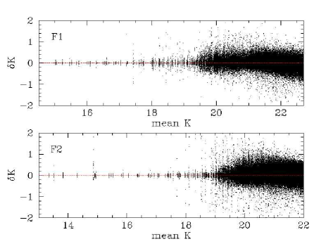
Figure 1: Photometric accuracy for the $K$-band data. Plotted are differences of individual epoch measurements with respect to their mean magnitudes. Only individual measurements with ALLFRAME $\sigma$ error smaller than 0.2 are plotted. At the bright end the limiting accuracy of $\pm 0.05$ mag can be seen. The variables are located where an excessive scatter with respect to the mean is present with both positive and negative excursions.

Not all the epochs were observed in photometric conditions. The $K$-band photometry was brought to the system of one of the photometric nights that had excellent seeing: epochs 1Ks07 and 2Ks10 for Fields 1 and 2, respectively, both observed on July 8, 2000. The zero point of $24.257\pm 0.042$ for that night has been derived from the observations of Persson et al. (persson+98 (1998)) standards supplied by ESO service observing (Rejkuba et al. rejkuba+01 (2001)). $J$- and $H$-band photometric zero points were derived using the observations of Persson standard stars obtained during the same night as the NGC 5128 observations in the corresponding filter (see Table 1) and their values are $24.737\pm 0.039$ and $24.626\pm 0.033$. For all three filters extinction coefficients measured by ESO observatory staff and reported on ISAAC web pages were assumed (0.06 for $K_{\rm s}$ and $J_{\rm s}$-band and 0.05 for $H$-band).

The quality of the photometry can be assessed from Figure 1 where we plot differences of individual epoch measurements vs. mean magnitudes. The mean magnitudes were calculated weighting the individual measurements with their photometric errors calculated by ALLFRAME:

$$\overline{K}=\frac{\sum\limits_{i=1}^{n}\frac{K_{i}}{\sigma^{2}_{i}}}{\sum\limits_{i=1}^{n}\frac{1}{\sigma^{2}_{i}}}$$ (1)

Only the stars with individual ALLFRAME $\sigma$ uncertainty measurements smaller than 0.2 mag are plotted. The limiting accuracy of our photometry at the bright end is $\pm 0.05$ mag, getting worse at faintest magnitudes. The region around K=20 has more scattered measurements than the mean. This is where most variable stars are found. The mean magnitude calculated with the above equation will, however, be overestimated (too bright) for variable stars with large amplitudes because brighter phases will typically get higher weights.

4 Search for variable stars

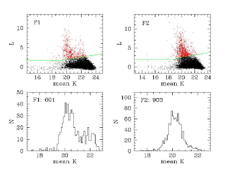
Figure 2: Variability index L vs. magnitude is plotted in the upper two panels for fields 1 (left) and 2 (right). Variable stars have higher index L values than non-variables and are found above the solid line. In the lower panels the magnitude distribution of variable stars is shown. The number of variables with at least 6 data points is also given.

Variable stars were identified using a procedure similar to the one described by Welch & Stetson (welch&stetson93 (1993)) and Stetson (stetson96 (1996)). First, we selected all the stars with mean of all photometric errors given by ALLFRAME, as measured on each individual epoch frame, smaller than 0.2 mag. We then required for each star to be detected on more than 5 frames and constructed variability indexes J, K and L, following the prescriptions by Stetson (stetson96 (1996); equations 1–3).

In particular the index J is used for single observations assuming $P_{i}=\delta^{2}_{i}-1$, where $\delta_{i}$ is a normalized residual of the measurement from the mean magnitude. The mean magnitude is calculated using a weighting with inverse square of the measurement error (weight $w_{i}$) according to equation 1.

The index J is a robust measure of the external repeatability relative to the internal precision. For single epoch observations containing only random noise its value tends to zero. For a physical variable it is a positive number. The index K is a robust measure of the kurtosis of the magnitude histogram and its value is fixed by the shape of the light curve, with K=0.9 for a pure sinusoid and K=0.798 for a Gaussian magnitude distribution, a limit approached when random measurement errors dominate over physical variation. Including the information about the variability and the shape of the light curve, Stetson defined the final variability index L as:

$$L=\left(\frac{JK}{0.798}\right)\left(\frac{\sum w_{i}}{w_{all}}\right)$$ (2)

The second term in this expression assigns an additional weight to stars with the highest number of measurements.

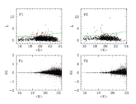
Figure 3: Variability index L vs. magnitude for simulated non-variable stars, i.e. those with light curve constant in time, is plotted in the upper two panels for fields 1 (left) and 2 (right). This diagram is used to decide the detection limit for the variable stars. In the lower panels scatter of the individual magnitude measurements around the mean magnitude is shown.

Figure 2 is a plot of the variability index L for all the stars in Field 1 and 2 in the left and right panels, respectively. The stars above the solid line (upper panels), plotted with slightly larger symbols, were searched for periodic variations. The limits that separate variable from non-variable sources were determined in the following way: in completeness simulations stars with constant magnitude light curves were added to the frames and their photometry and variability indexes were measured in identical way as for the programme stars. A similar plot of the variability index $vs.$ magnitude was used to decide on the separation line between the variable and non-variable stars (Figure 3). With the adopted variable star detection limits (solid lines in the upper panels) less than 2% of sources from these simulations are found above the lines. Note however, that at least some of these may have their light curves contaminated by a neighbouring variable star. Simulations necessary to evaluate the completeness of the variable star search are described below.

With such selection criteria 601 stars in Field 1 and 903 stars in Field 2 are found to be variable. Of these 536 and 878 had at least 10 measurements with individual errors smaller than 0.5 mag, and light curves were constructed for them.

5 Light curves and periods of LPVs

Fourier analysis of the $K$-band light curves was used to search for the periodic signal in the data in the range of $30<P<1700$ days. Only individual measurements with ALLFRAME uncertainty smaller than 0.5 mag were used. First, an initial guess of the period was obtained using a routine that calculates spectral power as a function of angular frequency ($\omega=2\pi f$; Lomb lomb (1976)):

$$P_{N}(\omega) = \frac{[\sum_{j}(K_{j}-\overline{K})\cos\omega(t_{j}-\tau)]^{2}}{2\sigma^{2}\sum_{j}\cos^{2}\omega(t_{j}-\tau)}$$ (3)

$$+ \frac{[\sum_{j}(K_{j}-\overline{K})\sin\omega(t_{j}-\tau)]^{2}}{2\sigma^{2}\sum_{j}\sin^{2}\omega(t_{j}-\tau)}$$

where $K_{j}$ and $\overline{K}$ are the individual and mean magnitudes, $\sigma$ is the variance, $t_{j}$ is the Julian Date (JD) of the measurement, and $\tau$ is defined as:

$$\tan(2\omega\tau)=\frac{\sum_{j}\sin 2\omega t_{j}}{\sum_{j}\cos 2\omega t_{j}}$$ (4)

The period obtained from the frequency with largest power corresponds to the most probable sinusoidal component. It was further improved with a non-linear least-square fitting of the function

$$K(t)=A\cos\left(2\pi\frac{(t-t_{0})}{P}\right)+B\sin\left(2\pi\frac{(t-t_{0})}{P}\right)+K_{0}$$ (5)

From this, the best fitting period (P), amplitude ($2\times\sqrt{A^{2}+B^{2}}$), mean magnitude ($K_{0}$), and phase ($t_{0}$) were obtained.

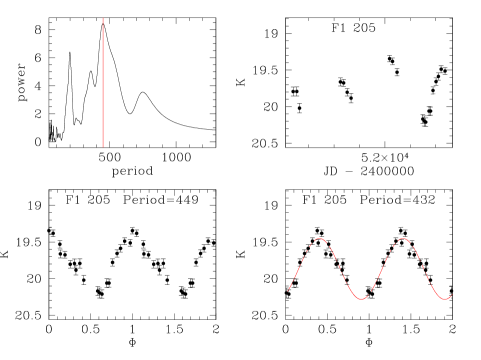
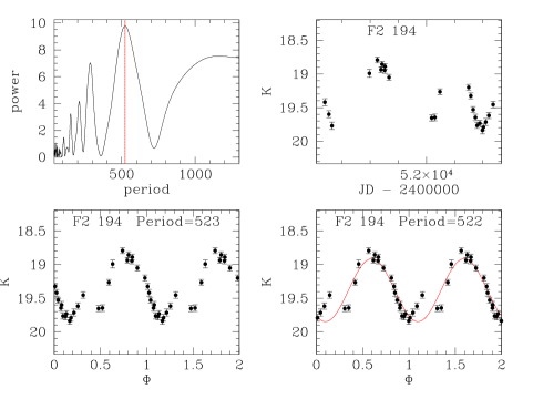
Figure 4: From left to right, top: periodogram and the original light curve in time domain; bottom: the light curve folded with the period obtained from the highest power frequency from the periodogram and the same light curve folded by the best period obtained from sine curve fitting. Each point in the phased light curves is plotted twice to emphasize the periodicity. Over the last light curve the fitting function is over-plotted. In the left panels the four diagrams are plotted for star #205 in Field 1 and in the right panels for star #194 in Field 2.

In optical passbands Miras often have asymmetric light curves, usually steeply rising to the maximum and with a shallower decline. In near-IR the variations are more regular and nearly sinusoidal (e.g. Whitelock et al. whitelock+00 (2000)). Hence a sine-wave gives a reasonable approximation to most of the LPVs.

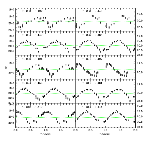
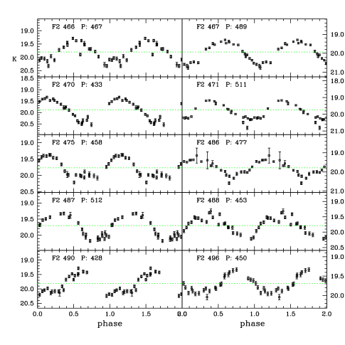
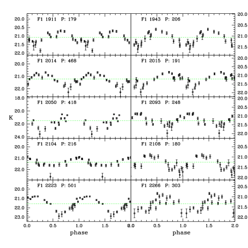
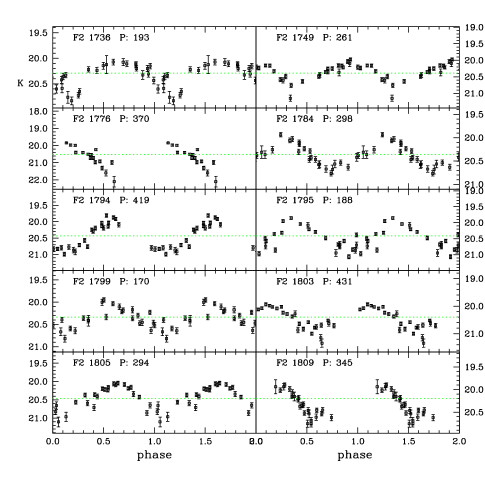
Figure 5: A sample of phased light curves for variables in both fields and with a range of mean magnitudes. Each point is plotted twice to emphasize the variability.

Table 2: Data for a sample of variables with light curves plotted in Fig. 5. The columns from left to right list: star ID, x and y position with respect to the reference epoch, the best fitting period, semi-amplitude, reduced $\chi^{2}$ of the sine-curve fit, significance of the period from Fourier analysis, single epoch $J$ and $H$-band magnitudes, and mean $K$-band magnitude from the sine-curve fit.

ID	x	y	N	P	A	$\chi^{2}$	signif	J	H	$<K>$
F1 286	279.230	67.260	20	197	0.247	9.20	0.550	20.96	20.24	19.87
F1 288	14.460	549.217	11	446	0.408	1.70	0.690	21.87	20.99	20.07
F1 294	124.558	330.030	20	449	0.387	5.20	0.160	21.07	20.23	19.95
F1 295	445.246	622.988	20	466	0.527	2.20	0.060	21.44	20.60	20.00
F1 296	395.486	18.707	19	194	0.217	2.50	0.260	20.78	20.11	19.84
F1 301	364.732	570.560	20	427	0.283	1.30	0.080	20.86	20.35	19.84
F1 304	169.875	226.678	20	458	0.483	1.50	0.050	21.13	20.32	20.05
F1 311	51.930	187.867	20	461	0.508	3.40	0.090	22.02	20.78	20.10
F1 312	326.187	501.922	20	510	0.436	2.20	0.160	21.16	20.43	20.07
F1 314	108.418	332.330	20	444	0.521	1.40	0.050	21.13	20.46	20.10
F1 1911	865.938	292.732	19	179	0.315	5.10	0.690	22.26	21.61	21.08
F1 1943	652.101	471.075	20	206	0.366	2.10	0.310	21.61	21.31	21.06
F1 2014	862.100	33.721	19	468	0.496	2.80	0.300	22.99	21.74	21.21
F1 2015	644.197	327.874	20	191	0.320	4.40	0.550	21.73	21.19	21.21
F1 2050	54.552	767.989	15	418	0.821	26.00	0.960	23.04	99.99	21.48
F1 2093	719.435	768.779	20	248	0.359	2.60	0.410	21.98	21.44	21.26
F1 2104	728.300	354.414	19	216	0.376	2.90	0.680	24.61	23.22	21.35
F1 2108	722.411	633.752	20	180	0.053	12.90	0.380	22.59	22.11	21.25
F1 2223	760.724	516.453	20	501	0.823	3.10	0.070	26.77	23.39	21.57
F1 2266	324.743	541.049	20	303	0.311	6.50	0.760	21.98	21.52	21.34
F2 466	497.668	115.838	24	467	0.381	7.50	0.060	21.03	20.99	19.80
F2 467	219.420	287.679	24	489	0.615	3.20	0.010	22.27	21.54	19.93
F2 470	413.810	765.776	24	433	0.514	2.50	0.010	20.82	20.00	19.88
F2 471	654.271	480.820	24	511	0.583	3.70	0.060	22.51	21.36	19.74
F2 475	388.723	379.739	24	458	0.327	4.70	0.040	20.66	20.03	19.76
F2 486	12.504	328.661	23	477	0.448	3.60	0.030	20.64	20.08	19.78
F2 487	215.930	745.931	24	512	0.432	2.90	0.040	21.57	20.91	19.70
F2 488	409.287	716.276	24	453	0.235	9.10	0.070	20.75	20.23	19.78
F2 490	597.413	11.477	24	428	0.377	5.70	0.030	21.41	20.70	19.81
F2 496	442.349	576.357	24	450	0.169	6.40	0.030	21.31	20.46	19.69
F2 1736	40.346	627.771	24	193	0.247	5.20	0.240	22.44	21.37	20.29
F2 1749	832.748	178.959	24	261	0.319	3.70	0.210	21.06	20.52	20.39
F2 1776	337.907	-7.156	16	370	0.607	11.10	0.660	24.63	22.32	20.51
F2 1784	711.917	559.903	24	298	0.330	2.00	0.030	21.84	21.10	20.36
F2 1794	491.605	75.748	23	419	0.488	4.00	0.020	22.75	21.87	20.43
F2 1795	405.954	409.103	24	188	0.394	10.60	0.410	21.90	20.98	20.41
F2 1799	575.492	194.880	24	170	0.231	5.80	0.240	22.02	21.10	20.33
F2 1803	786.644	606.898	24	431	0.405	5.30	0.080	21.38	20.70	20.40
F2 1805	359.442	396.001	24	294	0.356	4.30	0.090	21.24	20.57	20.46
F2 1809	849.471	740.460	24	345	0.386	3.30	0.060	21.56	20.96	20.19

Our code that determines the best fitting period was tested on a subsample of data on Mira variables published by Whitelock et al. (whitelock+00 (2000)). Their data are similar to ours, with 10–15 data points per star and photometric errors of the order of 0.05 mag in K. In 8 out of 10 cases we obtain the same period as Whitelock et al. In two cases our periods were significantly different (in one case we derived 74 days period with respect to the published value of 185 days and in the second case our period is 422 days where Whitelock et al. got 327 days), but the light curves folded with these periods looked as good or even smoother than the published light curves. In some cases is possible to obtain more than one acceptable period when there are less than $\sim 15$ data points. It is not clear however, if these stars really pulsate with two different periods or the insufficient data allow to derive such different periods due to aliases in the sampling of the data.

In Figure 4 we show two examples of a periodogram, the original light curve in time domain and the light curves folded with the period obtained from the highest power frequency from the periodogram and by a sine curve fitting. In a few cases there are evidences for the presence of the second period or a luminosity modulation in the data (e.g. star F2 #194 in Figure 4), but we have determined only the main period, because for most of the variables the data were not good enough for a more detailed analysis. Most of the times when a good period could be derived, the two periods were similar, but sometimes they differed by up to 20-30 days and both light curves were of acceptable quality. This illustrates that the accuracy of the derived periods and amplitudes varies considerably from one star to the next, depending on the number of observations, their individual errors and the stability of the light curve over the sampling interval.

It is interesting to note that some LPVs in the LMC with periods in excess of $\sim 420$ days, which appear to be rather bright for their periods when compared to other LPVs in the K-band or M_bol vs. $\log{\mathrm{P}}$ diagram, show a pronounced hump on the rising branch. These stars are tentatively identified as being in the Hot Bottom Burning stage of evolution on account of, for example, the strong Li apparent in some of their spectra (Glass & Lloyd Evans glass&evans (2003)). Star F2 #194 shows such a hump and it is lying 0.28 mag above the mean period-luminosity relation (Rejkuba 2003, in preparation). Reviewing the light curves of all the variables with $P>420$ days that are at least 0.3 mag brighter than the mean K-band magnitude at a given period, we found that approximately 1/3 ($\sim 15$ stars) present a similar hump. For some of the other 2/3 stars the light curve coverage is not sufficiently good to exclude the presence of a hump.

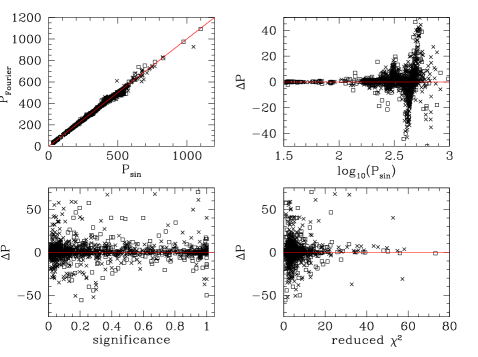
Figure 6: Comparison of periods derived through Fourier analysis (P_Fourier) and sine-curve fitting (P_sin) for variables in Field 1 (open squares) and Field 2 (crosses) and the dependence of the differences between the two methods on quality of the fit parameters: significance measures strength of the periodicity signal in Fourier analysis and reduced $\chi^{2}$ is a direct indicator of the quality of the sine-curve fit.

The comparison of the periods obtained through Fourier analysis and by a sine-curve fitting is shown in Figure 6. Variables in Field 1 are shown with open squares and those in Field 2 with crosses. The upper left panel is a direct comparison of the periods determined with the two methods, while the other panels show how the difference depends on period (upper right), on significance of the period obtained from Fourier analysis (lower left) and on reduced $\chi^{2}$ of the sine-curve fit. There is no significant difference between the two fields. The larger differences are more probable for variables with low $\chi^{2}$ of the sine-curve fit. This is an expected result due to the fact that not all the variables have strictly sinusoidal light curves. On the contrary, there is no strong dependence on the significance parameter which measures the strength of the peak in the periodogram (e.g. Figure 4). Significance is a smaller number for stronger (more significant) period. We have visually inspected all the variables folded with both periods and in cases where one of the two gave clearly much smoother light curve that period was retained, otherwise the final period is a mean of the two. A more quantitative accuracy of the periods, as well as the completeness of the detection of variables with a given period was derived using Monte Carlo simulations (see next section).

For 99 variable stars in Field 1 and 169 in Field 2 no acceptable periods could be obtained because of the non-sinusoidal variations, large errors combined with small amplitudes, periodicity outside our probed range ($30<P\la 1000$ day), presence of multiple periods, irregularity (cycle-to-cycle variations) in Miras or semiregulars, or absence of period (e.g. microlensing, background AGN or SN). More data are necessary to determine the nature of these variables. Among these are also LPVs that have periods longer than $\sim 1000$ days, for which our observations did not cover much more than 1 period and thus it was not possible to determine an accurate period.

The light curves for 437 variables in Field 1 and 709 in Field 2, for which we could determine periods, as well as the tables with the best fitting parameters for these stars, are presented only in the electronic version of the article. In Figure 5 we show a sample of light curves folded with the periods that are indicated in each panel. In the example there are bright and faint variables from both fields. Table 2 lists for these stars: ID number, x and y position with respect to the reference frame (1Ks07 and 2Ks10 for Field 1 and Field 2, respectively), number of epochs with magnitude measurements with $\sigma<0.5$, periods, semi-amplitudes ($\sqrt{A^{2}+B^{2}}$) as obtained from sine-curve fitting, reduced $\chi^{2}$ of the fits, significances, the $J$- and $H$-band magnitudes, and the $K$-band magnitudes from the sine-curve fit. Negative numbers for x and y positions mean that the star was out of the limits of the reference frame. The initial positions (x,y)=(1,1) correspond to $(\alpha,\delta)=(13^{h}26^{m}17\aas@@fstack{s}5,-42^{\circ}51\arcmin 03\aas@@fstack{\prime\prime}3)$ for Field 1 and to $(\alpha,\delta)=(13^{h}25^{m}18\aas@@fstack{s}0,-43^{\circ}09\arcmin 03\aas@@fstack{\prime\prime}0)$ for Field 2. This table is a subset of Tables 3 and 4 presented in the electronic version. Additionally, in the electronic version of the article we list all the raw $K$-band measurements for 1504 variables in both fields (Tables 7 and 8). Magnitude 99.99 and the error 9.99 denote that no measurement for that epoch was obtained. Here we give only first three lines of these tables.

Table 3: LPVs in Field 1. The columns from left to right list: star ID, x and y position with respect to the reference epoch, the best fitting period, semi-amplitude, reduced $\chi^{2}$ of the sine-curve fit, significance of the period from Fourier analysis, single epoch $J$ and $H$-band magnitudes and mean $K$-band magnitude. Magnitude 99.99 denotes that no measurement for that star was obtained.

F1 ID	x	y	N	P	A	$\chi^{2}$	signif	J	H	$<K>$
31	460.926	401.982	20	432.	0.513	21.10	0.650	19.00	18.16	17.37
53	107.785	832.967	19	448.	0.203	2.30	0.310	19.80	19.12	18.09
64	610.320	803.826	20	430.	0.202	18.50	1.000	18.92	18.57	18.36

Table 4: LPVs in Field2. The columns from left to right list: star ID, x and y position with respect to the reference epoch, the best fitting period, semi-amplitude, reduced $\chi^{2}$ of the sine-curve fit, significance of the period from Fourier analysis, single epoch $J$ and $H$-band magnitudes and mean $K$-band magnitude.Magnitude 99.99 denotes that no measurement for that star was obtained.

F2 ID	x	y	N	P	A	$\chi^{2}$	signif	J	H	$<K>$
35	115.155	-29.046	10	35.	0.978	226.70	0.940	18.65	18.42	18.48
49	41.708	172.990	10	988.	1.463	2.20	0.980	99.99	99.99	17.87
61	591.542	445.812	24	696.	0.180	1.70	0.300	19.56	18.77	18.41

Table 5: Additional variable stars in Field 1 for which periods could not be determined. The columns from left to right list: star ID, x and y position with respect to the reference epoch, single epoch $J$ and $H$-band magnitudes and mean $K$-band magnitude. Magnitude 99.99 denotes that no measurement for that star was obtained.

F1 ID	x	y	N	J	H	$<K>$
50	763.941	462.473	20	19.59	18.87	18.23
51	219.227	79.584	20	18.37	18.13	17.97
69	113.406	403.575	12	99.99	99.99	21.80

Table 6: Additional variable stars in Field 2 for which periods could not be determined. The columns from left to right list: star ID, x and y position with respect to the reference epoch, single epoch $J$ and $H$-band magnitudes and mean $K$-band magnitude. Magnitude 99.99 denotes that no measurement for that star was obtained.

F2 ID	x	y	N	J	H	$<K>$
5	110.132	451.042	17	99.99	18.79	15.51
25	111.583	-16.658	14	18.85	19.00	18.39
63	133.142	-27.505	9	19.02	18.60	18.96

Table 7: Individual measurements of the K-band magnitudes for all the red variable stars detected in Field 1. The columns from left to right list: star ID, x and y position with respect to the reference epoch, the reference epoch K-band magnitudes and errors and all the other individual K-band magnitudes and the errors of the measurements as given by ALLFRAME to which 0.04 mag calibration error have been added in quadrature. Magnitude 99.99 and the error 9.99 denote that no measurement for that star was obtained.

F1 ID	x	y	1Ks07 ($\sigma$)	1Ks01 ($\sigma$)	1Ks02 ($\sigma$)	1Ks03 ($\sigma$)	1Ks04 ($\sigma$)	1Ks05 ($\sigma$)	1Ks06 ($\sigma$)
			1Ks08 ($\sigma$)	1Ks09 ($\sigma$)	1Ks10 ($\sigma$)	1Ks11 ($\sigma$)	1Ks12 ($\sigma$)	1Ks13 ($\sigma$)	1Ks14 ($\sigma$)
			1Ks15 ($\sigma$)	1Ks16 ($\sigma$)	1Ks17 ($\sigma$)	1Ks18 ($\sigma$)	1Ks19 ($\sigma$)	1Ks20 ($\sigma$)
31	460.926	401.982	17.38 (0.09)	17.41 (0.08)	16.54 (0.08)	16.70 (0.06)	17.24 (0.09)	17.24 (0.06)	16.48 (0.07)
			17.37 (0.05)	17.50 (0.06)	17.54 (0.06)	17.49 (0.05)	17.26 (0.05)	17.85 (0.05)	18.04 (0.08)
			18.04 (0.08)	17.86 (0.09)	17.88 (0.09)	17.66 (0.05)	18.33 (0.11)	17.67 (0.07)
50	763.941	462.473	18.00 (0.08)	18.12 (0.05)	17.98 (0.05)	17.94 (0.04)	17.92 (0.07)	18.00 (0.05)	17.80 (0.05)
			17.85 (0.04)	18.04 (0.05)	18.03 (0.07)	18.09 (0.04)	17.99 (0.05)	18.08 (0.05)	18.19 (0.05)
			18.18 (0.05)	18.18 (0.04)	18.17 (0.06)	18.14 (0.05)	18.21 (0.04)	18.14 (0.05)
51	219.227	79.584	17.91 (0.04)	17.83 (0.04)	17.71 (0.06)	17.78 (0.05)	17.71 (0.05)	17.90 (0.04)	17.76 (0.05)
			18.12 (0.04)	18.06 (0.04)	18.07 (0.04)	18.23 (0.04)	18.18 (0.04)	18.24 (0.04)	18.29 (0.04)
			18.23 (0.05)	18.18 (0.04)	18.18 (0.05)	18.06 (0.04)	18.25 (0.05)	18.13 (0.04)

Table 8: Individual measurements of the K-band magnitudes for all the red variable stars detected in Field 2. The columns from left to right list: star ID, x and y position with respect to the reference epoch, the reference epoch K-band magnitudes and errors and all the other individual K-band magnitudes and the errors of the measurements as given by ALLFRAME to which 0.04 mag calibration error have been added in quadrature. Magnitude 99.99 and the error 9.99 denote that no measurement for that star was obtained.

F2 ID	x	y	2Ks10 ($\sigma$)	2Ks01 ($\sigma$)	2Ks02 ($\sigma$)	2Ks03 ($\sigma$)	2Ks05 ($\sigma$)	2Ks06 ($\sigma$)
			2Ks07 ($\sigma$)	2Ks08 ($\sigma$)	2Ks09 ($\sigma$)	2Ks11 ($\sigma$)	2Ks12 ($\sigma$)	2Ks13 ($\sigma$)
			2Ks14 ($\sigma$)	2Ks15 ($\sigma$)	2Ks16 ($\sigma$)	2Ks17 ($\sigma$)	2Ks18 ($\sigma$)	2Ks19 ($\sigma$)
			2Ks20 ($\sigma$)	2Ks21 ($\sigma$)	2Ks22 ($\sigma$)	2Ks23 ($\sigma$)	2Ks24 ($\sigma$)	2Ks04 ($\sigma$)
5	110.132	451.042	14.76 (0.04)	15.33 (0.14)	15.04 (0.15)	15.00 (0.12)	14.66 (0.05)	14.69 (0.04)
			14.68 (0.04)	14.68 (0.04)	14.69 (0.04)	15.37 (0.06)	15.41 (0.07)	15.50 (0.13)
			16.69 (0.13)	17.02 (0.16)	15.97 (0.28)	16.08 (0.18)	99.99 (9.99)	99.99 (9.99)
			99.99 (9.99)	99.99 (9.99)	99.99 (9.99)	99.99 (9.99)	99.99 (9.99)	14.73 (0.07)
25	111.583	-16.658	99.99 (9.99)	22.55 (0.25)	99.99 (9.99)	99.99 (9.99)	99.99 (9.99)	99.99 (9.99)
			99.99 (9.99)	99.99 (9.99)	99.99 (9.99)	17.57 (0.07)	18.26 (0.11)	16.74 (0.04)
			18.18 (0.21)	17.87 (0.11)	99.99 (9.99)	99.99 (9.99)	21.48 (0.34)	19.79 (0.24)
			20.17 (0.09)	21.46 (0.18)	18.18 (0.16)	19.47 (0.09)	19.93 (0.10)	19.98 (0.22)
35	115.155	-29.046	99.99 (9.99)	99.99 (9.99)	99.99 (9.99)	99.99 (9.99)	99.99 (9.99)	99.99 (9.99)
			99.99 (9.99)	99.99 (9.99)	99.99 (9.99)	17.02 (0.06)	99.99 (9.99)	16.71 (0.06)
			19.02 (0.27)	17.75 (0.18)	24.37 (6.32)	99.99 (9.99)	22.20 (0.49)	99.99 (9.99)
			20.37 (0.10)	21.65 (0.31)	18.49 (0.19)	99.99 (9.99)	21.58 (0.34)	19.99 (0.23)

It should be noted that while the large majority of the variables with the determined periods are long period variables with periods in excess of 100 days, there are 27 stars in Field 1 and 13 stars in Field 2 for which most probable periods were shorter than 51 days. However, the significance of these periods is in all cases is very low, with significance parameter $>0.8$ for all but two stars in Field 1 for which $\mathrm{signif}>0.65$. If the quoted periods are real, these stars could be Cepheids or some other kind of variables. Cepheids are expected to be found among younger populations in star forming regions like that present in our Field 1 (Rejkuba et al. rejkuba+01 (2001)). Unfortunately our sampling is not good enough to determine reliably the variability type from the light curve shape.

6 Completeness and contamination

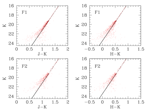
Figure 7: Completeness simulations: black dots distributed in a line that represents a mean RGB ridge line were added to all frames. Red dots scattered in the vicinity of that line are measured color-magnitude diagrams for these added stars. Stars simulated in the Field 1 crowding experiments are shown in the top panels and those in Field 2 are in the bottom panels.

The completeness of the photometric catalogue in the $J$, $H$ and $K$-bands was determined with crowding experiments. In ten different crowding experiments a set of stars with magnitudes uniformly distributed between $15.7<K<25.2$ was added to all the images after the appropriate re-scaling for the photometric zero point differences and shifting the stars so that they all fall at the same physical position in the sky coordinates. The $J-K$ and $H-K$ colors of the stars were chosen to follow a mean ridge line of the observed red giant branch (Figure 7). A realistic, observed, amount of Poissonian noise was added as well. The photometry was then re-calculated in the same way as described above.

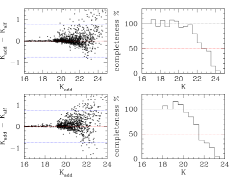
Figure 8: $K$-band photometric errors (left) and completeness (right): The simulations for Field 1 are in the upper and for Field 2 in the lower diagrams. Only stars that were measured at the same coordinates as the added stars and having $J$, $H$ and $K$-band magnitudes within $-0.75<\delta K<0.75$ (dotted lines on the left diagrams) are considered to be detected in the crowding experiments.

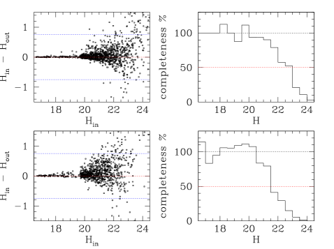
Figure 9: Same as Fig. 8 but for the $H$-band.

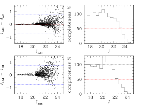
Figure 10: Same as Fig. 8 but for the $J$-band.

The results of these completeness experiments are shown in Figures 8, 9 and 10. Our photometry is complete more than 50% in the $K$ and $H$-bands for stars brighter than 22.5 and 21.5 mag for fields 1 and 2, respectively. These numbers for the $J$-band are 22.75 and 22.25 mag. Some bins have completeness larger than 100% due to false detections or migrations due to blends with original stars in the images. Note however, that we assume that the simulated star is detected only if its measured magnitude does not differ from the input value by more than 0.75 mag.

The left panels of Figures 8 to 10 show differences between input (added) and recovered (measured) magnitudes which is indicative of photometric errors at a given magnitude. From them it is evident that the stars fainter than 50% completeness have very large photometric errors. Apart from the completeness and photometric error estimations, these simulations were also used to determine criteria for the detection of variable stars. The results are summarized in Figure 3 and are described in Section 4.

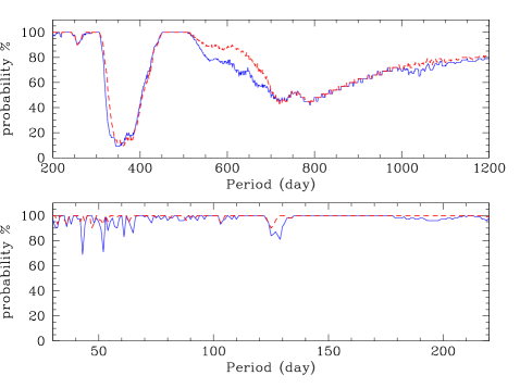
Figure 11: Probability of detecting a variable star as a function of period assuming an even distribution of measurements in phase (see text). The solid line is for Field 1 and the dashed line for observations of Field 2.

Further simulations of variable stars were used to gain information on the completeness and contamination in our LPV catalogue. Since the detection probability of a variable depends not only on the mean magnitude of the star, but also on period and amplitude, as well as on sampling distribution, different sets of simulations were carried out.

Dependence of the probability of the detection of a variable star with a given period on the actual distribution of the observations can be estimated with numerical simulations similar to those by Saha & Hoessel (saha&hoessel90 (1990)) and Bersier & Wood (bersier&wood02 (2002)). Given a period P and initial phase $\phi_{0}$ at the time $t_{0}$ of the first observation, the phase distribution can be calculated for our set of observations. Assuming that to detect a variable a uniform coverage in phase is required, with (1) at least two observations between phases 0 and 0.2, (2) at least two detections with phases between 0.2 and 0.5 and (3) at least two measurements with phases between 0.5 and 0.8, the resulting period detection probability is presented in Figure 11. Note that for a more realistic estimate this curve should be multiplied by the incompleteness corresponding to the mean magnitude of the variable. An additional factor in the period detection probability is the amplitude of the variable.

A better estimate of the detection probability for variables with given magnitudes, amplitudes and periods, can be obtained through simulations similar to the crowding experiments. In a series of such experiments we have added artificial variable stars with sinusoidal light curves with given periods, amplitudes and magnitudes. The magnitude range was chosen between $19.5<K<21.5$, similar to that of detected LPVs in NGC 5128 halo.

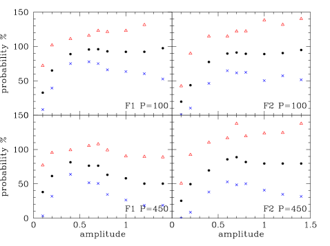
Figure 12: Probability of detecting a variable star as a function of amplitude for simulated variable stars with periods of P=100 day (top panels) and P=450 days (bottom panels). A simulated variable is considered to be detected only if $|\Delta mag|<0.75$ and $|\Delta P|\leq 25$. Simulations for Field 1 are on the left and those for Field 2 on the right. Different symbols are used for different magnitude bins: triangles for stars brighter than K=20.5, crosses for $K>20.5$ and filled dots for all the stars irrespective of their magnitude.

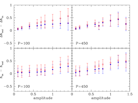
Figure 13: The difference between the detected and input amplitude (top panels) and the difference between the detected and input magnitudes (bottom panels) for simulated variables with periods of P=100 days (left) and P=450 days as a function of input amplitude. Simulations of Field 1 variables are shown with filled circles and those for Field 2 with open squares.

One series of completeness experiments tested our detection sensitivity to the amplitudes of variable stars. Variable stars with amplitudes between 0.1 and 1.4 mag for two fixed periods, 100 and 450 days were added to the original frames in 18 different crowding experiments for each field. In each single experiment all the variables had the same amplitude and period, but a range of magnitudes as mentioned above. In Figure 12 the percentage of detected variables, those with $-0.75\leq\Delta\mathrm{mag}\leq 0.75$ and $-25<\Delta\mathrm{P}<25$, as a function of amplitude is given for variables brighter than $K=20.5$ (triangles) and those with $K>20.5$ (crosses). Filled dots denote detection probability (or completeness) as a function of amplitude of variables for all the stars irrespective of their magnitudes. It is obvious from the fact that the bright stars have completeness higher than 100% that there is some migration of faint stars into the brighter magnitude bin.

This effect can also be seen in Figure 13 where we plot differences between detected and input magnitudes (bottom panels) and differences in detected and input amplitudes (top panels) as a function of input amplitude for all the variables. Simulations of Field 1 variables are plotted with filled dots and those of Field 2 with open squares. There is a systematic bias in the sense that we detect stars brighter than they are and with somewhat larger amplitudes. The magnitude of this bias is proportional to the amplitude of the variable. Partially this difference may be due to the way the mean output magnitude is calculated, but using different means still produces a slight bias. In order to have an estimate of bias independent of an a priori knowledge about the period and phase, because for some of the variables we could not determine periods and some stars in the field escaped detection as variable stars, we plot in Figure 13 differences in mean magnitudes as they get calculated by DAOMASTER task in DAOPHOT.

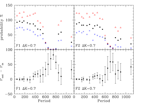
Figure 14: Probability of detecting a variable star as a function of period for simulated variable stars with amplitudes of $\Delta K=0.7$ mag for Field 1 (top left) and Field 2 (top right panel). Here a simulated variable is considered to be detected only if its detected magnitude did not differ from the measured value by more than 0.75 mag and if its measured period did not differ from the input one by more than $\pm 25$ days. Bottom panels show difference in measured and input periods for variables as a function of period.

From Fig. 12 it is obvious that most of the large amplitude variables ($\Delta K>0.3$) will be detected for stars with shorter periods. Our variable star catalogue is highly incomplete for stars with amplitudes of 0.2 mag or smaller, irrespective of period. The absolute value of which percentage of variables with a given amplitude will be detected for longer period LPVs depends strongly on our choice of detection criterion. If we consider that a variable star is detected only if its measured period does not deviate from the input one by $\pm 25$ days, detection probability at P=450 days is between 50 and 80%, but if we allow a larger uncertainty in period detection, our catalogue is more complete.

In order to see what is the completeness of our catalogue with respect to period of variable stars and how precise our period measurements are we performed a series of experiments in which we have added to our frames artificial variable stars with sinusoidal light curves with typical amplitudes for LPVs ($\Delta K=0.7$ mag) and magnitudes in the range between $19.5<K<21.5$, similar to that of detected LPVs in NGC 5128 halo. Periods were chosen at  50 day interval, ranging from 50 to 1100 days. In particular 365 day and 182 day period variable stars were also added. Photometry of all the added stars was performed in the same way as before and the light curve parameters calculated as explained above. The measured detection probability as a function of period is presented in Figure 14. Again we plot the detection probability for all the simulated stars with a given period with filled dots. Open triangles and crosses are used for bright ($K<20.5$) and faint ($K>20.5$) stars, respectively. In plotting the top panels of Fig. 14 we assumed a variable star to be detected only if (i) its mean magnitude did not differ from the input mean magnitude by more than 0.75 mag, (2) if it was detected in at least 10 frames, and (iii) if its measured period did not differ from the input period by more than $\pm 25$ days. Due to this last restriction there is an almost zero probability to detect variables with periods around 700-800 days. However, in our catalogue there are variables with these periods. In fact the bottom panels of Figure 14 show a dependence of the difference between measured and input periods as a function of input period. From this it is obvious that for the variables with periods in the range between 700 and 800 days we systematically overestimate their periods by as much as 50-100 days. In the top panels these variables are considered non-detections. Periods for variables with periods longer than 800 days can be determined more accurately. An additional potential systematic error could come from period aliasing. Our observations do not span time continuously. Rather, they are grouped in three to six month windows with inter-window gaps of 200 to 320 days. Thus, it is possible that stars with actual periods in the range 175 – 200 days were assigned periods of order of one year, because only alternate maxima fell within our observing windows.

7 Conclusions

We have presented the first catalogue of variable stars in a giant elliptical galaxy. 1504 red variables were detected in two halo fields of NGC 5128 (Centaurus A) covering 10.46 arcmin square. For 1146 variables with at least 10 good measurements we have determined periods, amplitudes and mean K-band magnitudes using Fourier analysis and non-linear sine-curve fitting algorithms. Periods, amplitudes and $JHK$ photometry are given for 1146 long period variables. Additionally, individual K-band measurements are given for all the red variables.

Our extensive completeness simulations show that periods determined for these long period variables are accurate to $\pm 25$ days except in the range of 700-800 days where the accuracy does not exceed $\pm 50$ to 100 days. Additionally there may be a few cases where an aliasing period may introduce a larger error due to less than optimal sampling.

Mean magnitudes of variable stars are measured to be brighter than simulated mean magnitudes by up to $\sim 0.3$ mag and this brightening depends on the amplitude of a variable stars. Typically for variables with amplitudes smaller than $\sim 1$ mag measured mean magnitudes are very similar to the input magnitudes. This brightening is partially due to the way the mean magnitude is calculated. For constant light curve stars in the same magnitude range as the variable stars ($19.5<K<21.5$) there is no bias, i.e. the difference between measured and input magnitude is consistent with zero.

Our variable star catalogue is close to 90% complete for short period long amplitude variables. For variable stars with variability amplitudes of 0.2 mag or smaller detection probability is 50% or smaller. There is a strong dependence of the detection probability on the period of a variable. Our simulations show that most variable stars with periods in the range of 700-800 days will have their periods strongly biased toward larger values, overestimating the period by as much as 50-100 days.

In the next paper the complete analysis of the period and amplitude distribution as well as their dependence on the magnitude and color of the variable stars will be presented. The comparison with long period variables in the Milky Way and the Magellanic Clouds will be made.

- (1) Bersier, D. & Wood, P.R., 2002, AJ, 123, 840
- (2) Bertelli, G., Bressan, A., Chiosi, C., Fagotto, F. & Nasi, E., 1994, A&AS, 106, 275
- (3) Fassett, C.I. & Graham, J.A., 2000, ApJ, 538, 594
- (4) Feast, M.W., Robertson, B.S.C., Catchpole, R.M., et al., 1982, MNRAS, 201, 439
- (5) Frogel, J.A. & Whitford, A.E., 1987, ApJ, 320, 199
- (6) Frogel, J.A. & Elias, J.H., 1988, ApJ, 324, 823
- (7) Frogel, J.A. & Whitelock, P.A., 1998, AJ, 116, 754
- (8) Glass, I.S. & Lloyd Evans, T., 2003, MNRAS, in press
- (9) Guarnieri, M.D., Renzini, A. & Ortolani, S., 1997, ApJ, 477, L21
- (10) Habing, H.J., 1996, A&A Rev., 7, 97
- (11) Harris, G.L.H. & Harris, W.E., 2000, AJ, 120, 2423
- (12) Harris, G.L.H., Harris, W.E. & Poole, G.B., 1999, AJ, 117, 855
- (13) Kennicutt, R. C., 1998, ARA&A 36, 189
- (14) Kerschbaum, F. & Hron, J., 1992, A&A, 263, 97
- (15) Kerschbaum, F. & Hron, J., 1994, A&AS, 106, 397
- (16) Kholopov, P.N. et al., 1985, General Catalogue of Variable Stars 4th edn., Nauka Publishing House, Moscow (GCVS)
- (17) Liu, M.C., Graham, J.R. & Charlot, S., 2002, ApJ, 564, 216
- (18) Lomb, N.R., 1976, Ap&SS, 39, 447
- (19) Malin, D.F., Quinn, P.J. & Graham, J.A., 1983, ApJ 272, L5
- (20) Marleau, F.R., Graham, J.R., Liu, M.C. & Charlot, S., 2000, AJ, 120, 1779
- (21) Mei, S., Silva, D.R. & Quinn, P.J., 2001, A&A, 366, 54
- (22) Mould, J.R., Ridgewell, A., Gallagher, J.S. III et al., 2000, ApJ, 536, 266
- (23) Persson, S.E., Murphy, D.C., Krzeminski, W., Roth, M. & Rieke, M.J., 1998, AJ, 116, 2475
- (24) Rejkuba, M., 2001, A&A, 369, 812
- (25) Rejkuba, M., 2002, PhD thesis, P. Universidad Católica de Chile
- (26) Rejkuba, M., Minniti, D., Bedding, T. & Silva, D.R., 2001, A&A, 379, 781
- (27) Rejkuba, M., Minniti, D., Courbin, F. & Silva, D.R., 2002, ApJ, 564, 688
- (28) Saha, A. & Hoessel, J.G., 1990, AJ, 99, 97
- (29) Soria, R., Mould, J.R., Watson, A.M., et al., 1996, ApJ 465, 79
- (30) Stanford, S.A., Eisenhardt, P.R.M. & Dickinson, M., 1995, ApJ, 450, 512
- (31) Stetson, P.B., 1996, PASP, 108, 851
- (32) Stetson, P.B., 1994, PASP, 106, 250
- (33) Stetson, P.B., 1987, PASP, 99, 191
- (34) Tonry, J. & Schneider, D.P., 1988, AJ, 96, 807
- (35) Tonry, J.L. & Schechter, P.L., 1990, AJ, 100, 1794
- (36) Welch, D.L. & Stetson, P.B., 1993, AJ, 105, 1813
- (37) Whitelock, P., Marang, F. & Feast, M., 2000, MNRAS, 319, 728
- (38) Wood, P.R., Bessell, M.S. & Fox, M.W., 1983, ApJ, 272, 99