On the efficiency of the Ultra Steep Spectrum tecnique in finding High-z Radiogalaxies
Abstract
In the last three decades, the Ultra Steep spectrum tecnique has been exploited by many groups since it was demonstrated that radio sources with very steep spectra (; ) are good tracers of high-z radio galaxies (HzRGs; ). Though more than HzRGs have been discovered up to now with this tecnique, little is known about its real effectiveness, as most of the ongoing searches still have incomplete follow-up programs. By selecting a new appropriate sample of USS sources from the MRC survey, the true searching efficiency of the USS tecnique has been quantitatively demonstrated for the first time in this paper. Moreover it was compared with that of an optical search of HzRGs based on a simple cut of the galaxies r-band magnitude distribution. When no bias other than the radio-spectrum steepness is applied, the USS tecnique may be up to times more efficient in selecting HzRGs with respect to an optical search. Nevertheless, when the search is limited to objects fainter than the POSS-II plates (), the USS tecnique is still times more efficient ( vs. ). For an optical search to reach a comparable efficiency it is necessary to select objects fainter than , but this implies that about half of the HzRGs are lost because of the imposed magnitude bias. The advantage of the USS tecnique is that a search efficiency is already reached at the POSS-II plates limit, where all the optical identification work is done without telescopes. However, this tecnique has the drawback that up to of the HzRGs of the sample are lost simply because of the applied spectral index bias. Interestingly, the introduction of a strong angular-size bias such as can double the searching efficiency irrespectively of the adopted tecnique, but only in the case that no optical bias has been introduced first.
keywords:
Radio galaxies , SurveysPACS:
98.54.G , 01.30.R1 Introduction
The efforts made in the last three decades to build large samples of Ultra Steep Spectrum (USS) radio sources have been justified by a supposed high efficiency of this tecnique to select very distant galaxies. Its effectiveness derives from a combination of the (high) redshift of the source with an intrinsic steepening of the radio spectrum at high frequencies. In practice, distant sources with concave radio spectra, will have steeper spectral indices than similar sources at low redshift. It has been demonstrated (Tielens et al. 1979, Blumenthal & Miley 1979) that the introduction of a radio spectrum steepness criterium implied a large decrease of the fraction of object with optical counterparts identified on the POSS-I (). This was consistent with the steeper spectrum sources being, on average, at high redshifts. Surveys at low frequencies (MHz) are particularly efficient in selecting radiogalaxies and have at least two benefits. One is that quasars contribute by no more than to the total number counts ; the second is that most of the detected energy arises from the radio-lobes with negligible contribution from the sources cores, where Doppler boosting can play an important role. In principle, as differential sources counts at MHz show an excess over the Euclidean prediction in the range Jy, a survey with such limiting fluxes should provide an unbiased sample of objects and a high fraction of high-redshift radiogalaxies (henceforth HzRGs) as well. The difficulty in picking-up these object arises from the large number of candidates to be targeted at optical; given the low intrinsic fraction of high-z objects in a radio survey, the majority of the targets will reveal to be unwanted foreground objects. It is thus of fundamental importance to introduce some kind of bias to reduce the number of HzRGs candidates.
In low-frequency radio surveys (MHz), the extragalactic sources with steep spectra () are a small fraction of the total, typically no more than %, and this fraction lowers down to % if more drastic cuts () are adopted. Starting from large unbiased radio catalogs is thus essential to build-up conspicuous samples of USS sources. Selecting USS sources implies that the imaging/spectroscopic optical follow-up work is limited to a relatively small number of candidates, giving us higher chances of success. In addition, radio searches are not affected by dust/obscurement effects, contrarily to what happens with pure optical searches. The drawback is that the resulting sample may be not representative of the entire population of the high-z objects, since studies conducted on complete samples of classical double sources (Blundell et al. 1999) showed that sources with steep spectra at low frequencies tend to be smaller and more powerful with respect to sources with ’normal’ spectra. With the advent of the new all-sky surveys (WENSS, NVSS, FIRST), unprecedently deep and large USS samples have been selected (De Breuck et al. 2000), either to increase the number stastistics and to detect intrinsically fainter sources. These surveys virtually should have pushed the steep spectrum tecnique to its limit, in the sense that they are deep enough for any AGN class object to be detected even at the highest redshifts (). Nevertheless, despite much has been published about the radio surveys and the properties of the USS sources, very few claims do exist about the real effectiveness of this tecnique in selecting HzRGs. The temptative estimate given by some authors (van Breugel et al. 1997), though quite realistic, resulted from such a mix of radio/optical/NIR biases that makes it impossible to disentangle the role of the radio spectrum steepness itself. The organization of the paper is as follows: the properties of the existing samples of USS sources are resumed in Sect. 2 and the procedure used to derive a quantitative estimate of the real effectiveness of the USS tecnique is described in Sect.3. Conclusions are summarized in Sect.4.
2 USS samples from the literature; radio and optical properties
Up to now many USS samples have been selected, as many groups started extensive searches for very distant radiogalaxies using the radio-spectrum steepness as a selection criterium. In practice, all the existing radio catalogs in the range of frequencies MHz have been combined together to build USS sources samples. When building an USS sample, it is common practice to perform a positional cross-correlation of the sources detected in a low-frequency survey with those of a high-frequency one, in order to calculate a two-point spectral index. The selection frequency plays an important role in determining the efficiency of finding HzRGs. An outstanding example is the sample of 4C sources (Baldwin & Scott 1973), whose counterparts were searched on the MHz survey of Williams et al. (1966) by imposing the criterium . Twelve out of sources were found to be associated with Abell clusters with median redshift . These low-frequency USS sources are almost exclusively found in rich clusters, and are often associated with extended radio haloes or relic structures. Syncrotron losses of an ageing population of emitting electrons, confined by the dense intra-cluster medium, may explain the unusual steepeness of their spectrum. On the other hand, radio spectra of the high-z USS sources do steepen at high frequencies due to a combination of syncrotron/inverse compton losses and the redshift. At low frequencies, a flattening of their spectrum may result from syncrotron-self absorption occurring in the sources hot-spots.
| Sample | Limit Flux (Jy) | bias | bias | Sources |
|---|---|---|---|---|
| 4C-BS | ; | none | ||
| 4C-T | ; | none | ||
| 6C | ||||
| RC | ; | none | ||
| WV | ||||
| B3.2 | ||||
| MRC | none | |||
| TN | ; | none | ||
| WN | ; | none | ||
| MP | ; | none | ||
| Leiden | Variousa | none |
Though most of the USS sources samples from the literature have almost complete radio data, their optical follow-up programmes are often far from being completed. Deriving statistical results from these samples is not straightforward, as different selection criteria (e.g. spectral index, sources LAS, optical magnitude) were often mixed together to maximize the searching efficiency but the net effect on the final samples is not well understood. Moreover, the biases introduced by these criteria are almost impossible to disentangle as we usually deal with small samples spanning small ranges in radio luminosity. This is the reason why very few quantitative claims do exist on the real effectiveness of the USS tecnique in selecting high-z galaxies up to date. In Tables 1 and 2, we summarize radio and optical data of the most representative USS sources samples available from the literature.
| Sample | %ID on POSS-I | (arcsec) | % | % | ||
|---|---|---|---|---|---|---|
| 4C-BS | ||||||
| 4C-T | ||||||
| 6C* | ||||||
| RC | ||||||
| WK | ||||||
| B3.2 | ||||||
| MRC | ||||||
| TN | ||||||
| WN | ||||||
| MP | ||||||
| Leiden | n.a. |
From Table 2 it results that the existing USS samples are very effective in selecting very distant galaxies with roughly half of the objects being indeed radiogalaxies with redshift . It should be noted, however, that apart the 6C sample which has complete optical information, the above statistics are derived from subsamples which represent only a small fraction of the original samples. In addition, some ’hidden’ selection criteria (e.g. a K-band magnitude lower-limit), sometimes adopted to better discard foreground objects (e.g. De Breuck et al 2000), make it difficult to assess the real efficiency of such a radio tecnique.
With the only exception of the 3CR, no other unbiased radio samples are available with complete radio and optical data as well. Nevertheless it is interesting to compare the properties of some unbiased samples with those of poorly biased samples such as the B3-VLA.
| Survey | Frequency | Flux Density | # Sources | No | Biases | ||
|---|---|---|---|---|---|---|---|
| 3CR | MHz | Jy | none | ||||
| MRC | MHz | Jy | none | ||||
| B2/1Jy | MHz | Jy | none | ||||
| B3-VLA | MHz | Jy | |||||
From Table 3, it results that the radio steepness bias, eventually coupled with an angular-size bias, increases the efficiency of selecting radio galaxies at redshifts . Excluding the 3CR that contains only one RG with , the other low-frequency radio surveys contain typically no more than of HzRGs. One of the most studied samples is the B2/1Jy (Allington-Smith 1982) which contains radio sources with Jy. Out of radiogalaxies, have redshift information. This subsample has a median redshift and median spectral index . It contains only USS sources with , of which one is a radiogalaxy with and the other is unidentified. This sample includes RGs with , five with and one with ; thus out of () B2/1Jy sources are indeed high redshift galaxies, though none of them would have been selected on the basis of the radio spectral index criterium. In the case of the B2/1Jy sample, the radio steepness criterium clearly fails to select the high-z radiogalaxies but, interestingly, if an angular-size cut like is introduced, a total of objects are selected, including RGs with . Thus, the angular-size bias itself would select all the B2/1Jy HzRGs with a global efficiency of .
The B3-VLA sample (Vigotti et al. 2003; in preparation) has a mild spectral index bias, coupled with a relatively strong angular-size bias; for this reason it may be considered half way between the usual USS samples and the unbiased samples. For a typical low-frequency radio sample, a spectral index cut like roughly implies half of the sources to be filtered out, while an angular-size bias such as only implies of the sources to be excluded (see also Table 1). Since low-frequency radio samples all have small median sizes (), we can argue that the angular-size bias adopted for the B3-VLA sample has little influence on the final content of HzRGs. This result suggests that the expected increase of the fraction of galaxies is not seen in the B3-VLA sample mainly because of the mild spectral index cut adopted.
3 Testing the effectiveness of the USS tecnique
At present there are no radio surveys with complete radio and optical data that can be used to assess the validity of the USS searching technique (see Tables 2 and 3). The ideal sample to test the real effectiveness of this tecnique would be that with complete radio and optical information. Unfortunately, apart the well known 3CR and B2/1Jy samples, no other survey has a follow-up programme that reached such a degree of completion. While for the 3CR sample the very high limiting flux density virtually prevents any HzRG to be selected, in the case of the B2/1Jy sample the poor number statistics prevents any statistically significant result to be derived.
3.1 The MRC/1Jy sample - radio and optical data
Actually, the only available low-frequency sample, free of selection biases and with a reasonably complete radio/optical dataset is the MRC/1Jy sample selected by McCarthy et al.(1996) from the Molonglo Reference Catalogue (Large et al. 1981). In the following it will be shown that, despite a substantial redshift incompleteness toward the faintest magnitudes, this sample can provide a dataset five times larger than the B2/1Jy sample, well suited for statistical studies. VLA maps at cm with typical resolution of exist for all the MRC galaxies which allow a precise morphological classification. Kapahi et al. (1998) listed the flux densities at MHz and GHz for radio galaxies drawn from the MRC/1Jy sample. When the flux density at GHz was not available, the value at GHz was reported. To build-up a homogenous sample, essential for the present study, it was decided to get NVSS (Condon et al. 1998) flux densities for all the MRC radiogalaxies in order to re-define the spectral indices as . This criterium closely resembles the original one adopted to select the MRC USS sample (, see Table 1). As the median spectral index for the MRC galaxies resulted to be , a ’canonical’ spectral index bias has been chosen to select this newly defined MRC USS sample. McCarthy et al. (1996) reported a identification fraction of the MRC radio sources down to the magnitude. To date, r-band magnitudes are available for of these MRC galaxies and redshift information is available for of these galaxies (McCarthy et al. 1996, Kapahi et al. 1998 and references therein). Thus, complete radio and optical data actually exist for a subsample of MRC radiogalaxies. Hereinafter the two samples of and RGs will be referred to as MRCB and MRCC respectively.
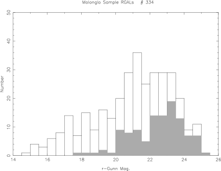
The r-band magnitude distribution for the MRCB sample has a median value and it is shown in Figure 1. For comparison the median magnitude of the MRCC sample is . A redshift incompleteness toward the faint end is evident from Figure 1 as the sources lacking of redshift data preferentially lie close to the MRC optical identification limit, as confirmed by their significantly higher-than-average median magnitude ().
The redshift incompleteness of the MRCB sample can be assessed as follows. After dividing the sample into two subsamples, respectively fainter and brighter than the median magnitude, for each subsample the ratio between the number of RGs with and without redshift is calculated. In the bright sample, only of the RGs have no measured redshift but the fraction increases to for the faint sample, indicating a substantial incompleteness. The MRCC sample redshift distribution is shown in Figure 2. The median redshift is , but the objects fainter than the median magnitude , have a significantly higher redshift .

A crucial point for our analysis is that the redshift incompleteness of the MRCB sample at faint levels could imply the MRCC sample has a lower-than-average content of USS sources. The fact that the median magnitude of the RGs with no redshift data is similar to that of the known USS samples () could favour the above hypothesis. Nevertheless it can be demonstrated that this is not the case. According to our criterium, out of the RGs are also USS sources (). A direct comparison between the USS content of the MRCB and the smaller MRCC sample gives respectively the values of and ; thus, the redshift incompletenss of the MRCB sample is unlikely to affect the MRCC sample, since only of USS sources are lost.
3.2 HzRGs and USS sources in the MRCC sample
The MRCC sample contains RGs with redshift ( of the total), of which are USS sources. As the sample contains USS sources, if no other selection criterium than the spectral index bias is applied, the efficiency would be . This relatively high efficiency of the USS tecnique has the drawback that a significant fraction of genuine targets are lost; in this case, out of HzRGs ().
3.3 The optical magnitude - radio spectral index plane
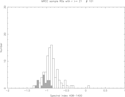
As the digitized POSS-I or POSS-II plates are normally used for the first step of any optical identification programme, let us assume that all the optical counterparts have been identified down to . In the case of the MRCC sample, this implies a reduction of the number of HzRGs candidates by a factor of , with a consequent increase of the searching efficiency (now instead of ). At the same time, the efficiency of the USS technique also increases, reaching the considerable value of . Thus, at least in the case of the MRCC sample, we conclude that by simply selecting the USS sources fainter than one is guaranteed that half of the candidates will be HzRGs. To study the effect of different radio and optical biases on the MRCC sample, the radio spectral indices were plotted against the r-band magnitudes (see Figure 3). For comparison, data for the MRC galaxies without redshift are also plotted.

Since all the MRCC HzRGs are fainter than , this value may be taken as a good starting point for our analysis. If the RGs with are considered, a total of objects are selected; their spectral indices distribution is shown in Figure 4.
If only the USS sources would be targeted at optical, out of objects would result to be HzRGs, with a net searching efficiency . Note however that HzRGs ( of the total) would be lost as they are not USS sources. In contrast, if no radio spectrum criterium is adopted, there would be sources to observe at optical ( times more telescope time); all the HzRGs would be selected, resulting in a final selection efficiency . Thus, when the search is limited to targets fainter than magnitude, the USS searching technique is about times more efficient with respect to the optical search. As expected, the overall telescope time investment is largely in favour of the radio selection technique. To increase the efficiency of the optical search, the number of candidates to be imaged could be reduced by adopting a more drastic bias in magnitude.Lowering the optical threshold down to reduces the sample to objects (see Figure 5).
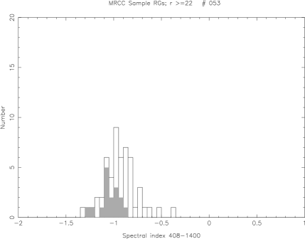
With respect to the original MRCC sample, the number of objects is now reduced by a factor of four. Observing all these objects at optical ensures that out of the HzRGs contained in the MRCC sample are selected, with a net efficiency ( HzRGs are lost because of the magnitude limit). On the other hand, this subsample contains only USS sources, out of which are HzRGs. The USS technique thus has a remarkable efficiency but HzRGs ( of the total) are lost as they are not USS sources.
Note that while tends to increase when going to fainter magnitudes, remains almost constant around the value . Pushing the optical magnitude limit toward fainter values is not recommended as the size of the resulting sample (and its statistical strenght) drastically reduces and the fraction of HzRGs that are lost rapidly increases. For example, going to implies that only RGs are retained. The optical search reaches its peak efficiency with HzRGs being selected. However out of HzRGs () are lost as they are brighter than . At the same time, the USS technique selects HzRGs from a total of sources, with an efficiency . In this case out of HzRGs ( of the total) are lost. Despite the expected loss of some HzRGs, the USS technique is again more efficient with respect to the optical search by about percent.
3.4 The role of the angular-size bias
Most of the existing USS samples were derived without imposing any angular-size bias (see Table 1). Nevertheless, even choosing unresolved sources in low-frequencies surveys such as Texas or WENSS, automatically implies an intrinsic angular cut-off of and respectively. The samples completeness may be affected by other factors. In the case of the Texas survey, the complicate behaviour of the beam of the interferometer (Douglas et al. 1996) implies that the resulting TN sample is only complete down to the survey nominal flux density limit (De Breuck et al. 2000).

To increase the efficiency of the USS tecnique some authors introduced a angular-size criterium to filter-out most of the foreground objects. Since the most distant objects should be among the faintest and the smallest ones, an angular size bias should increase the efficiency of finding HzRGs. The choice of the optimal cut-off value is quite arbitrary; though there are very few cases of known HzRGs with large angular sizes (4C 23.56 at has ), most of them have (Carilli et al. 1997). Adopting more drastic criteria such as , implies a reduction by of the total number of sources but it can lead to the exclusion of several good candidates. It can be demonstrated that the angular-size bias alone is effective to filter-out relatively bright and thus nearby objects. In fact, if all the MRCC objects are considered without any magnitude and size limit (see Fig.6), the optical search efficiency is only , while the USS efficiency is , four times higher. If a bias is introduced, we found that and become almost twice as large (respectively and ).
| Mag. Bias | Size Bias | # Sources | HzRGs lost | HzRGs lost | ||
| none | none | none | ||||
| none | ||||||
| none | none | |||||
| none | none | |||||
| none | ||||||
| none |
On the other hand, the angular-size bias seems to have little or no effect when an optical bias has been formerly introduced. Let us consider the previously discussed case when the MRCC objects fainter than were selected. Again, if the above angular-size bias is applied, the efficiency of the optical and USS searches remains almost unchanged, being respectively and . This is somewhat expected since an optical bias like already selects those objects wich are, in principle, more distant and thus smaller.
To conclude, the introduction of a strong angular size bias such as , increases the efficiency in selecting HzRGs by a factor of two, independently on what searching technique is adopted (optical or radio). Note that the same increase of efficiency is obtained by selecting only those objects with , irrespectively of their angular size. The relative efficiencies of the optical and radio searching techniques as a function of different cuts in the magnitude and angular size distribution are summarized in Table 4.
4 Conclusions
In this paper the real efficiency of the Ultra Steep Spectrum tecnique in finding HzRGs is quantitatively demonstrated for the first time since this radio tecnique was introduced. Moreover, an updated view is given of the radio/optical properties of the most representative USS sources samples and the role of the spectral index and angular-size biases is discussed. A new sample of USS sources was selected from the MRC/1Jy sample (McCarthy et al. 1996; Kapahi et al. 1998). Since the available radio dataset is not homogeneous, the radio flux densities from the NVSS were used to re-calculate the spectral indices as and a conservative radio-spectrum bias was adopted to select the USS sources. Our USS sample thus consists of MRC radiogalaxies with complete optical and radio data and it was used as a benchmark to study how different radio and optical biases do affect a homogeneous population of radio galaxies. It was found that the USS searching technique is much more efficient in finding HzRGs than a conventional search based on the optical magnitudes of the RGs. If no restrictions are applied to the optical magnitudes distribution, the USS technique may be up to times more efficient than the optical one. The obvious drawback is that a substantial fraction of the HzRGs population may be lost because of the introduced radio spectrum bias. When considering galaxies fainter than magnitude , the radio-steepness criterium guarantees that of the candidates are indeed HzRGs; this has to be compared with a mere of the optical search. Going to fainter magnitudes leads to a progressive increase of the efficiency of the optical search, that reaches its peak at with a notable efficiency (see Table 4). Note, however, that half of the HzRGs of the sample are lost when applying such a strong optical bias. Interestingly, the efficiency of the USS tecnique remains stable around irrespectively of the applied optical magnitude bias; going to fainter magnitudes only increases the fraction of genuine HzRGs that are lost (up to at ). To conclude, even at the faintest optical magnitudes here studied, the USS tecnique is more efficient of an optical search in selecting HzRGs, with the remarkable difference that the radio tecnique already reaches a efficiency at the magnitude limit. The advantage of the optical search is that, at least up to , a much smaller fraction of HzRGs is lost with respect to the radio tecnique ( instead of ). The introduction of an angular-size bias to the MRCC sample, such as , increases the searching efficiency by a factor of two, irrespectively of the searching tecnique adopted. However this additional bias has little or no effect when a magnitude bias such as is applied first to the sample, as it is the case when the first step of the optical identification program is done on the digitized POSS-I or POSS-II plates. This evidence suggests that the angular-size bias, sometimes used as an additional criterium, plays a secondary role with respect to the spectral index bias. This is also suggested by the finding that the USS samples actually adopting the steepest spectral index criterium and no angular-size bias (TN and WN samples; ) are those with the highest efficiencies in finding HzRGs.
5 Acknoledgements
The author wants to thank the anonymous referee and the NA editor, Prof. G. Setti, for their useful comments and suggestions on the manuscript.
References
- [1] Allington-Smith, J.R. 1982, MNRAS 199, 611 (1982MNRAS.199..611A)
- [2] Baldwin, J., Scott, P. 1973, MNRAS 165, 259 (1973MNRAS.165..259B)
- [3] Blumenthal, G., Miley, G.K., 1979, A&A, 80, 13 (1979A&A....80...13B)
- [4] Blundell, K., Rawlings, S., Eales, S.A., Taylor, G.B., Bradley, A.D. 1998, MNRAS 295, 265 (1998MNRAS.295..265B)
- [5] Blundell, K., Rawlings, S., Willot, C., 1999, AJ 117, 677 (1999AJ..117...677B)
- [6] Bremer, M.,N., Rengelink, R., Sauders, R., Röttgering, H.J.A., Miley, G.K., Snellen, I.A.G., Observational Cosmology with the New Radio Surveys, 1998, Bremer, M.,N., Jackson, N., Perez-Fournon, I., (eds.). Dordrecht: Kluver, p.165 (1998ocnr.conf..165B)
- [7] Carilli, C.L., Röttgering, H.J.A., van Ojik, R., Miley, G.K., van Breugel, W.J.M. 1997, ApJS 109, 1 (1997ApJS..109....1C)
- [8] Chambers, K.C., Miley, G.K., van Breugel, W.J.M., Huang, J.S. 1996, ApJS 106, 215 (1996ApJS..106..215C)
- [9] Condon, J.J., Cotton, W.D., Greisen, E.W., Yin, Q.F. et al., 1998, AJ 115, 1693 (1998AJ....115.1693C)
- [10] De Breuck, C., van Breugel, W.J.M., Röttgering,H.J.A., Miley, G., 2000, A&AS 143, 303 (2000A&AS..143..303D)
- [11] Douglas, J.N., Bash, F., Bozyan, F.A., Torrence, G.W., Wolfe, C., 1996, AJ 111, 5 (1996AJ....111.1945D)
- [12] Griffith, M.R., Wright, A.E., 1993, AJ 105, 1666 (1993AJ....105.1666G)
- [13] Kapahi, V.K., Athreya, R.M., van Breugel, W.J.M., McCarthy, P.J., Subrahmanya, C.R. 1998, ApJS 118, 275 (1998ApJS..118..275K)
- [14] Jarvis, M., Rawlings, S., Willot, C., Blundell, K., Eales, S., Lacy, M.; The Hy-Redshift Universe: Galaxy Formation and Evolution at High Redshift, 1999, Andrew J., Bunker and van Breugel, W.J.M. (eds.). Berkeley: ASP Conference Proceedings, p.90 (1999hrug.conf...90J)
- [15] Hales, S.E.G.,Baldwin, J.E., Warner, P.J. 1993, MNRAS 263, 25 (1993MNRAS.263...25H)
- [16] Large, M.I., Mills, B.Y., Little, A.G., Crawford, D.F., Sutton, J.M. 1981, MNRAS 194, 693 (1981MNRAS.194..693L)
- [17] McCarthy, P.J., Kapahi, V.K., van Breugel, W.J.M., Subrahmanya, C.R. 1990, AJ 100, 1014 (1990AJ....100.1014M)
- [18] McCarthy, P.J., van Breugel, W.J.M., Kapahi, V.K., Subrahmanya, C.R. 1991, AJ 102, 522 (1991AJ....102..522M)
- [19] McCarthy, P.J., Kapahi, V.K., van Breugel, W.J.M., Persson, S.E., Athreya, R.M., Subrahmanya, C.R. 1996, ApJS 107, 19 (1996ApJS..107...19M)
- [20] Parijskij, Yu.N., Bursov, N.N., Lipovka, N.M., Soboleva, N.S., Temirova, A.V. 1991, A&AS 87, 1 (1991A&AS...87....1P)
- [21] Pedani, M., Grueff, G., 1999, A&A 350, 368 (1999A&A...350..368P)
- [22] Rengelink, R.B., Tang, Y., de Bruyn, A.G., Miley, G.K., Bremer, M. et al. 1997, A&AS 124, 259 (1997A&AS..124..259R)
- [23] Röttgering, H.J.A., Lacy, M., Miley, G.K., Chambers, K.C., Saunders, R. 1994, A&AS 108, 79 (1994A&AS..108...79R)
- [24] Röttgering, H.J.A., van Ojik, R., Miley, G.K., Chambers, K.C. et al. 1997, A&A 326, 505 (1997A&A...326..505R)
- [25] Slingo, A. 1974a, MNRAS 166, 101 (1974MNRAS.166..101S)
- [26] Slingo, A. 1974b, MNRAS 168, 307 (1974MNRAS.168..307S)
- [27] Tielens, A. , Miley, G., Willis, A. 1979, A&AS, 35, 153 (1979A&AS...35..153T)
- [28] Van Breugel, W.J.M.,de Breuck, C., Röttgering, H.J.A., Miley, G., Stanford, A., Looking deep in the Southern Sky, 1999, Proc. of ESO/Australia workshop, Morganti, R., Couch, W.J. (eds.) (1997ldss.conf...V)
- [29] Wieringa, M.H. 1991, Ph.D. Thesis, Leiden University (1991PhDT.....241W)
- [30] Wieringa, M.H., Katgert, P. 1992, A&AS 93, 399 (1992A&AS...93..399W)
- [31] Williams, P.J.S., Kenderline, S., Baldwin, J.E. 1966, MNRAS 70, 53 (1966MNRAS..70...53W)