THE C IV MASS DENSITY OF THE UNIVERSE AT REDSHIFT 5 

Abstract

In order to search for metals in the Lyman $\alpha$ forest at redshifts $z_{\rm abs}>4$, we have obtained spectra of high signal-to-noise ratio and moderately high resolution of three QSOs at $z_{\rm em}>5.4$ discovered by the Sloan Digital Sky Survey. These data allow us to probe to metal enrichment of the intergalactic medium at early times with higher sensitivity than previous studies. We find 16 C IV absorption systems with column densities $\log N{\rm(C~{}IV)}=12.50-13.98$ over a total redshift path $\Delta X=3.29$. In the redshift interval $z=4.5-5.0$, where our statistics are most reliable, we deduce a comoving mass density of C³⁺ ions $\Omega_{\rm C~{}IV}=(4.3\pm 2.5)\times 10^{-8}$ (90% confidence limits) for absorption systems with $\log N{\rm(C~{}IV)}\geq 13.0$ (for an Einstein-de Sitter cosmology with $h=0.65$). This value of $\Omega_{\rm C~{}IV}$ is entirely consistent with those measured at $z<4$; we confirm the earlier finding by Songaila (2001) that neither the column density distribution of C IV absorbers nor its integral show significant redshift evolution over a period of time which stretches from $\sim 1.25$ to $\sim 4.5$ Gyr after the big bang. This somewhat surprising conclusion may be an indication that the intergalactic medium was enriched in metals at $z\gg 5$, perhaps by the sources responsible for its reionization. Alternatively, the C IV systems we see may be associated with outflows from massive star-forming galaxies at later times, while the truly intergalactic metals may reside in regions of the Lyman $\alpha$ forest of lower density than those probed up to now.

1 INTRODUCTION

Efforts to probe the universe at ever higher redshifts have continued to gather momentum in the last few years. The Sloan Digital Sky Survey (SDSS) has led to the discovery of many quasars (QSOs) at $z>5$ (Fan et al. 2003 and references therein) and searches for normal star forming galaxies at these epochs have been equally successful, reaching $z\simeq 6.6$ (Hu et al. 2002; Yan, Windhorst, & Cohen 2003; Lehnert & Bremer 2003; Kodaira et al. 2003; Stanway, Bunker, & McMahon 2003). One of the main goals of all of these studies is to identify the time when the baryons in the intergalactic medium (IGM) were reionized by the light of the first stars and galaxies. The spectra of SDSS QSOs at $z\lower 2.15277pt\hbox{$\;\buildrel>\over{\sim}\;$}6$ are essentially black at wavelengths below the Lyman $\alpha$ emission line, a finding which has been interpreted as the signature of the trailing edge of the cosmic reionization epoch (e.g. Becker et al. 2001; Fan et al. 2002; Cen & McDonald 2002; White et al. 2003). Yet, the recent detection by the Wilkinson Microwave Anisotropy Probe (WMAP) of a large optical depth to Thomson scattering, $\tau_{e}=0.17\pm 0.04$, suggests that the universe was reionized at higher redshifts, $z_{\rm ion}=17\pm 5$ (Kogut et al. 2003; Spergel et al. 2003). If confirmed, this would be an indication of significant star-formation activity at very early times.

Beyond $z\simeq 4$, the information provided by the Lyman $\alpha$ forest itself becomes progressively more difficult to interpret because of the severe line blending and rapidly increasing optical depth which leave little signal in QSO spectra. In order to follow the evolution of the IGM to earlier times we have to rely on the metal lines associated with the Lyman $\alpha$ forest, the most common of which is the C IV $\lambda\lambda 1548.2041,1550.7812$ doublet. The standard for this work has been set by the analysis of Songaila (2001). By bringing together measurements from the spectra of 32 QSOs, Songaila was able to follow the evolution of the column density distribution of C IV absorbers, $f(N)$, over the redshift interval $1.5\leq z\leq 5$. In today’s ‘consensus’ cosmology, $\Omega_{\rm M}=0.3$, $\Omega_{\Lambda}=0.7$, $H_{0}=65$ km s^-1 Mpc^-1, this redshift range corresponds to a time interval from 4.5 to 1.25 Gyr after the big bang. The surprising result is that no evolution can be discerned in $f(N)$, nor in its integral which gives the mass density of C³⁺ ions, $\Omega_{\rm CIV}$ (expressed as a fraction of the critical density). Taken at face value, this finding may suggest that most of the IGM metals were already in place at the highest currently observable redshifts, and may thus point to an early enrichment epoch by outflows from low-mass subgalactic systems (Madau, Ferrara, & Rees 2001). Alternatively, the density of C³⁺ ions may not reflect in a simple way the overall density of metals in the IGM if, for example, late winds from massive Lyman break galaxies are the source of the strongest C IV absorption systems (Haehnelt 1998; Adelberger et al. 2003). It then becomes extremely important to push the study of the C IV ‘forest’ to higher redshifts not only to distinguish between these different chemical evolution scenarios, but also to understand the mechanisms by which metals are distributed from their stellar birthplaces and mixed within the IGM.

The sample of QSOs analyzed by Songaila (2001) was assembled as the first results from the SDSS were beginning to appear in the public domain, and therefore included relatively few objects at $z>5$. Consequently, her statistics on $f(N)$ and $\Omega_{\rm CIV}$ are least secure at the highest redshifts. In this paper, we add to Songaila’s work with deep observations of three recently discovered SDSS QSOs, all at $z>5$, obtained with the aim of improving the statistics of the column density distribution by: (a) increasing the sample, (b) reaching to lower values $N$(C IV), and (c) considering the likely corrections due to sample incompleteness. Our main conclusion is that we confirm the previously reported lack of evolution in $\Omega_{\rm CIV}$. The observations are described in §2, while in §3 we provide measurements of the C IV absorbers detected in the three QSO spectra. In §4 and §5 we analyze our sample and compare our findings with those reported by Songaila (2001). Finally, in §6 we briefly discuss possible interpretations of these results and their implications for the origin of C IV absorption at high redshifts.

2 OBSERVATIONS AND DATA REDUCTION

The spectra of the three QSOs were recorded with the Echelle Spectrograph and Imager (ESI; Sheinis et al. 2000) on the Keck II telescope in January and February of 2002; relevant details of the observations are collected in Table 1. With its combination of high efficiency at red and near-IR wavelengths, wide wavelength coverage (from 4000 Å to 1 $\mu$m), and moderately high resolution ($R\simeq 6500$) ESI is well suited to the aims of the present work.

The QSOs SDSS 0231$-$0728 (Anderson et al. 2001) at $z_{\rm em}=5.421$ and SDSS 0836+0054 (Fan et al. 2001b) at $z_{\rm em}=5.803$ were observed with a 0.75 ${}^{\prime\prime}~{}$wide entrance slit, which projects to approximately four $11.5$ km s^-1 pixels in the dispersion direction. For SDSS 1030+0524 (Fan et al. 2001b) at $z_{\rm em}=6.305$, a 1 ${}^{\prime\prime}~{}$wide entrance slit was employed. For all observations the slit was aligned at the parallactic angle, and the airmass was always less than 1.5 . Reference spectra of internal lamps were used for wavelength calibration and flat-fielding. Observations of the smooth spectrum white dwarf star G191B2B, obtained on each night, provided a template for dividing out the numerous telluric absorption lines which mar ground-based spectra in the far red and near-IR; they were also used to place the QSO spectra on an absolute flux scale (Massey et al 1988; Massey & Gronwall 1990).

The individual two-dimensional ESI images (recorded with exposure times of either 1200, 1800, or 2700 s) were processed using custom IDL routines written by one of us with the specific aim of maximising the accuracy of background subtraction; this is often the limiting factor in deep spectroscopy of faint sources at long optical wavelengths, where line emission from the night sky dominates the signal.

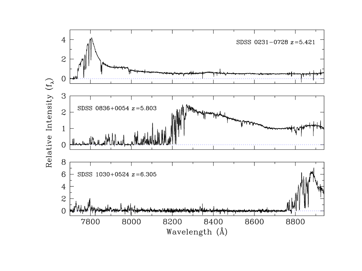
Figure 1: Portions of the ESI spectra of the three QSOs observed in this study.

After flat-fielding, wavelength calibration and background subtraction, the individual one-dimensional spectra were mapped onto a common, vacuum heliocentric, wavelength scale before being added together to produce the final spectra, shown in Figure 1.

Corresponding variance spectra are also produced by the data reduction software. In column (6) of Table 1 we list typical values of the signal-to-noise ratio (S/N) in the QSO continuum in the wavelength regions where we searched for C IV doublets (see §3). Generally, the S/N is highest near the Lyman $\alpha$ emission line and decreases at longer wavelengths. In the two best observed QSOs, SDSS 0836+0054 and SDSS 1030+0524, the long exposure times (see column (5) of Table 1) resulted in S/N $\lower 2.15277pt\hbox{$\;\buildrel>\over{\sim}\;$}60$ and 40 respectively at wavelengths between Lyman $\alpha$ emission and 9000 Å. The resolution of the spectra, as measured from the widths of night sky emission lines, is $\sim 1.3$ Å FWHM ($\simeq 45$ km s^-1), sampled with $\sim 4$ wavelength bins for the QSOs SDSS 0231$-$0728 and SDSS 0836+0054 (and $\sim 30$% coarser for SDSS 1030+0524). With their combination of high S/N and resolution, the spectra used in this study are some of the best published of very high redshift QSOs, as can be appreciated from Figure 1 and from the last column of Table 1 which lists the $3\sigma$ detection limits for the rest frame equivalent widths of unresolved C IV lines.

The final steps in the data reduction involved correcting for atmospheric absorption by diving the QSO spectra by that of the smooth spectrum star (suitably normalized), and fitting the QSO continuum. Both steps were carried out using the Starlink software package DIPSO. The end result are normalised QSO spectra which could then be searched for C IV absorption.

3 C IV ABSORPTION LINES AT HIGH REDSHIFT

The spectra of the three QSOs were visually inspected independently by two of us for pairs of absorption lines with the correct separation and relative strengths to be C IV doublets. After various trials (including the simulations described in §5 below), we decided to restrict the search to two wavelength regions. The first region extends from the Lyman $\alpha$ emission line of the QSO longward to 8940 Å, near the onset of the atmospheric A-band. The second region is a relatively small gap, between 9200 and 9300 Å, which is free of strong atmospheric absorption and sky emission lines (and, for this reason, is being exploited in narrow-band searches for high redshift Lyman $\alpha$ emitters—see, for example, Hu et al. 2002). The reason for restricting ourselves to these wavelength intervals is that at other wavelengths strong atmospheric absorption reduces significantly the S/N achieved. Even with the best efforts to divide out the atmospheric lines, our sensitivity to C IV absorption is much reduced here; simulations confirmed that we could only recover the strongest C IV doublets, and with only partial success. Although this choice effectively imposes a limit of $z_{\rm abs}\leq 5.0$ to the redshift range over which we can study C IV, we nevertheless prefer to concentrate our analysis on regions where our detection limit is relatively uniform. The simulations described in §5 show that in these regions we are essentially complete for C IV absorption lines with rest frame equivalent width $W_{0}\geq 40$ mÅ.

Once C IV doublets had been identified, their normalized line profiles were fitted with theoretical Voigt profiles using the VPFIT package. VPFIT deconvolves the composite absorption profiles into the minimum number of discrete components and returns for each the most likely values of redshift $z_{\rm abs}$, Doppler width $b$ (km s^-1), and column density $N$(C IV) (cm^-2) by minimizing the difference between observed and computed profiles. The profile decomposition takes into account the instrumental point spread function of ESI. Vacuum rest wavelengths and $f$-values of the C IV transitions are from the recent compilation by Morton (2003). We now briefly discuss each QSO in turn.

3.1 SDSS 0231$-$0728

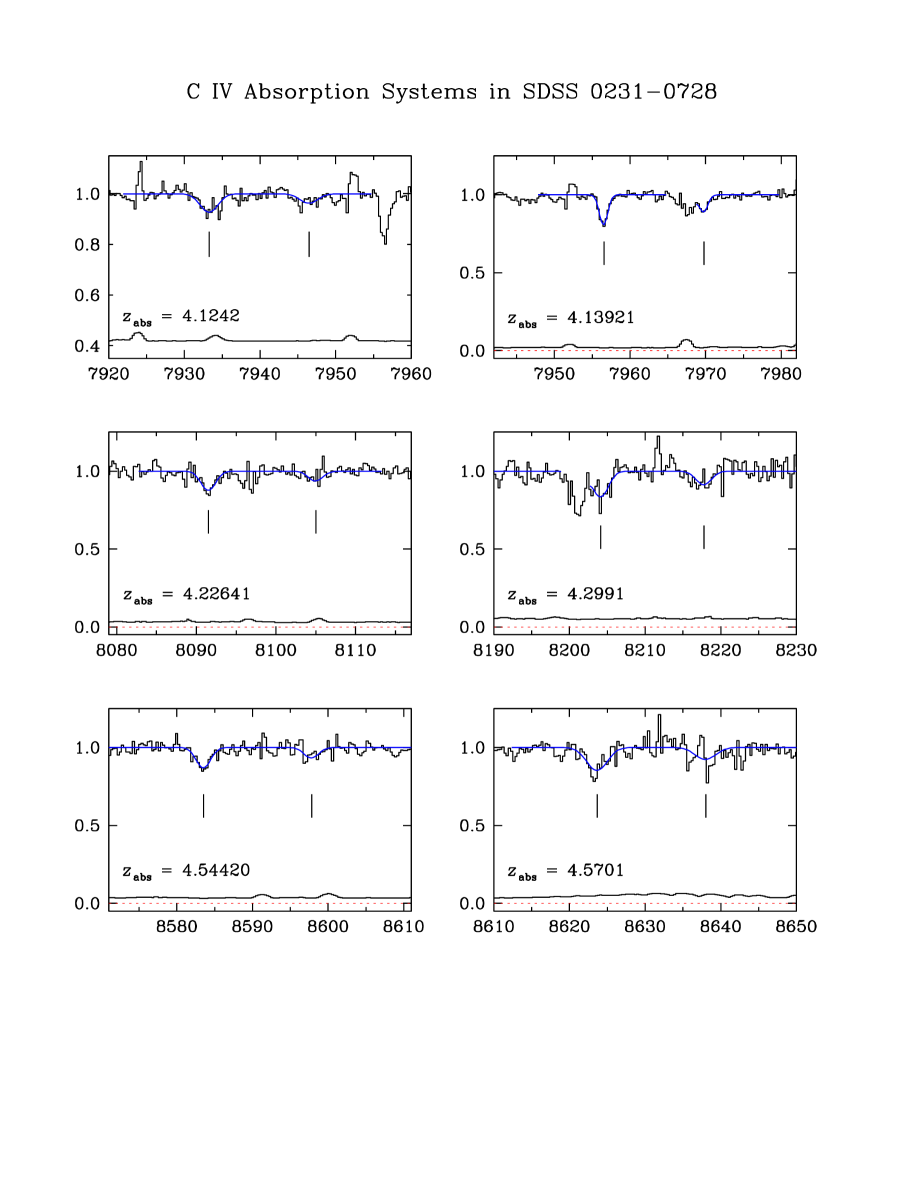
Figure 2: Normalised absorption profiles (histograms) of C IV systems in SDSS 0231$-$0728. The $y$-axis is residual intensity, while the $x$-axis gives the observed wavelength in Å. The thin continuous lines show theoretical profiles produced by VPFIT with the parameters listed in Table 2. Vertical tick marks indicate the positions of the C IV $\lambda\lambda 1548.2041,1550.7812$ doublet lines. The line near the zero level shows the $1\sigma$ error spectrum. The weak C IV system at $z_{\rm abs}=4.1242$ (top left-hand panel) is shown for clarity on an expanded $y$-scale; in this case the error spectrum has been offset by $+0.4$ in $y$.

The peak of the Lyman $\alpha$ emission line in this QSO, at 7806 Å, corresponds to $z_{\rm abs}$=4.0420 for C IV$\lambda 1548.2041$; thus, we can search for C IV doublets in the redshift intervals $4.0420\leq z_{\rm abs}\leq 4.7745$ (7806–8940 Å) and $4.9424\leq z_{\rm abs}\leq 5.0070$ (9200–9300 Å). We find eight C IV systems, listed in Table 2 and reproduced, together with their profile fits, in Figure 2. The two systems labelled ‘Marginal’ in Table 2 are cases where we do not feel confident of the identifications because the weaker member of the doublet is affected by residuals in the sky subtraction.

3.2 SDSS 0836+0054

The higher redshift of this QSO (the peak of the Lyman $\alpha$ emission line is at 8270 Å) means that we can only search for C IV doublets over a more restricted redshift range, from $z_{\rm abs}=4.3417$ to 4.7745 (8270–8940 Å), as well as $4.9424\leq z_{\rm abs}\leq 5.0070$ (9200–9300 Å). We find seven C IV absorption systems, one of which consists of (at least) three separate components (see Table 3 and Figure 3).

3.3 SDSS 1030+0524

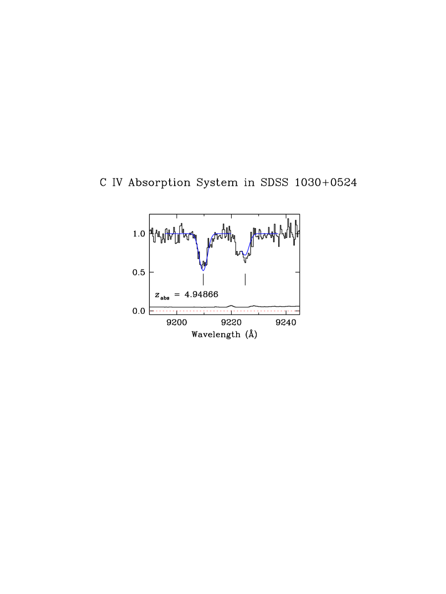
Figure 4: Normalised absorption profile (histogram) of the only C IV system detected in SDSS 1030+0524. The $y$-axis is residual intensity. The thin continuous line shows the theoretical profile produced by VPFIT with the parameters listed in Table 4. Vertical tick marks indicate the positions of the C IV $\lambda\lambda 1548.2041,1550.7812$ doublet lines. The line near the zero level shows the $1\sigma$ error spectrum.

This is the highest redshift QSO among the three studied here; with the peak of the Lyman $\alpha$ emission line occurring at 8880 Å, we have only 60 Å of clear continuum before the onset of the atmospheric A-band. We find no C IV systems in this narrow redshift interval ($z_{\rm abs}$= 4.7357 – 4.7745), although one is detected between 9200 and 9300 Å, at $z_{\rm abs}$= 4.94866 (see Table 4 and Figure 4).

The errors quoted in Tables 2, 3, and 4 are the $1\sigma$ estimates returned by VPFIT on the basis of the error spectra provided to the fitting program. These spectra are shown as a line near the zero level in each panel of Figures 2, 3, and 4, and can be seen to be a reasonable representation of the rms deviations from the continuum level away from strong sky lines (the residuals from the subtraction of the sky lines can sometimes amount to many times the estimated value of sigma, reflecting systematic, rather than random, errors in the sky subtraction). However, VPFIT does not take into account the possibility that what we see as an individual C IV line is actually an unrecognized blend of more than one absorption component. This is a common problem in the analysis of interstellar (or in this case intergalactic) absorption lines, made worse here by the relatively coarse resolution of ESI. Specifically, the ESI point spread function of FWHM = 45 km s^-1 corresponds to an instrumental Doppler parameter $b_{\rm instr}=27$ km s^-1. This is significantly larger than the typical $b$-values of C IV lines at lower redshifts ($z=2-3$); for example Rauch et al. (1996) reported $b_{\rm median}$(C IV) $=10.6$ km s^-1, while Ellison et al. (2000) found $b_{\rm median}$(C IV) $=13$ km s^-1, both from higher resolution ($5-8$ km s^-1 FWHM) spectra than those considered here.

There are several hints in our data that we may underestimating the complexity of the C IV absorption lines. First, the values of $b$ we deduce are all larger than the median values at $z=2-3$, as referenced above. We consider it much more likely that this is an effect due to the limited spectral resolution of our data, rather than a genuine redshift evolution in the intrinsic line widths. Second, unrecognized velocity structure may be the reason why the fits to the some of our C IV systems are poor (examples are the $z_{\rm abs}$ = 4.685 complex and the $z_{\rm abs}$ = 4.99695 system in Figure 3). In general, the result of blending several components into one unresolved feature is an underestimate of the column density, because narrow saturated components, if they exist, could easily be masked by broader ones (Nachman & Hobbs 1973). The $z_{\rm abs}$ = 4.66874 system in Figure 3 is an example where the C IV doublet ratio is indicative of saturation. VPFIT converges to a value of $b_{\rm CIV}$ very much less than $b_{\rm instr}$; therefore, in this case $b_{\rm CIV}$ remains undetermined and we quote in Table 3 a lower limit to $N$(C IV) based on the equivalent width of $\lambda 1550.7812$, the weaker member of the doublet, assuming no saturation. In conclusion, given the limited resolution of ESI, the values of $N$(C IV) derived here should strictly be considered as lower limits, a point which we shall keep in mind in the interpretation of the results.

4 THE MASS DENSITY OF C IV

The mass density of C IV ions, expressed as a fraction of the critical density today, $\rho_{\rm crit}=1.89\times 10^{-29}\,h^{2}$ g cm^-3, can be calculated as (e.g. Lanzetta 1993)

$$\Omega_{\rm CIV}=\frac{H_{0}\,m_{\rm CIV}}{c\,\rho_{\rm crit}}\int Nf(N){\rm d}N,$$ (1)

where $H_{0}=100\,h$ km s^-1 Mpc^-1 is the Hubble constant, $m_{\rm CIV}$ is the mass of a C IV ion, $c$ is the speed of light, and $f(N)$ is the number of C IV absorbers per unit column density per unit absorption distance $X(z)$. This last quantity is used to remove the redshift dependence in the sample: absorbers with constant comoving space density and constant proper size have a constant number density per unit absorption distance along a line of sight. In a flat Friedmann universe with matter and vacuum density parameters today $\Omega_{M}$ and $\Omega_{\Lambda}$, the absorption distance is given by

$$X(z)=\int_{0}^{z}dz^{\prime}\,{(1+z^{\prime})^{2}\over[\Omega_{M}(1+z^{\prime})^{3}+\Omega_{\Lambda}]^{1/2}}={2\over 3\Omega_{M}}\,\{[\Omega_{M}(1+z)^{3}+\Omega_{\Lambda}]^{1/2}-1\}.$$ (2)

In the case of an Einstein-de Sitter universe with ($\Omega_{M},\Omega_{\Lambda})=(1,0)$, we recover the standard expression $X(z)=2[(1+z)^{3/2}-1]/3$ (Tytler 1987).

Our total sample consists of 16 or 12 C IV systems, depending on whether we include the marginal detections or not. Although these absorbers span a factor of $\sim 30$ in column density, from $\log N$(C IV) = 12.50 to 13.98 (see Tables 2, 3 and 4), our completeness drops to below 50% for $\log N$(C IV) $\lower 2.15277pt\hbox{$\;\buildrel<\over{\sim}\;$}13.0$ (§5). It is not possible to determine $f(N)$ on the basis of such limited statistics. However, we can still deduce an estimate of $\Omega_{\rm CIV}$ using the approximation

$$\int Nf(N){\rm d}N=\frac{\sum_{i}N_{i}{\rm(C~{}IV)}}{\Delta X}$$ (3)

(e.g. Storrie-Lombardi, McMahon, & Irwin 1996), where $\Delta X$ is the total absorption distance covered by our spectra. In the following we will adopt an Einstein-de Sitter cosmology for comparison with earlier work; then $\Delta X$ is given by

$$\Delta X=\frac{2}{3}~{}\sum_{j}[(1+z_{j}^{\rm max})^{3/2}-(1+z_{j}^{\rm min})^{3/2}].$$ (4)

The summation in equation (4) is over the $j$ redshift intervals $\Delta z$ where we can detect C IV systems in our data; as explained in §3, we have two such intervals in each of the three sight-lines to the QSOs in Table 1. With $h=0.65$, equations (1) and (3) then lead to:

$$\Omega_{\rm CIV}=1.75\times 10^{-22}~{}\frac{\sum_{i}N_{i}{\rm(C~{}IV)}}{\Delta X}.$$ (5)

For the error in $\Omega_{\rm CIV}$, $\delta\Omega_{\rm CIV}$, we adopt the estimator proposed by Storrie-Lombardi et al. (1996):

$$(\delta\Omega_{\rm CIV})^{2}=\frac{\sum_{i}[N_{i}{\rm(C~{}IV)}]^{2}}{\left[\sum_{i}N_{i}{\rm(C~{}IV)}\right]^{2}}.$$ (6)

For consistency with Songaila (2001), in what follows we quote errors which correspond to formal 90% confidence limits, that is $\delta\Omega_{\rm CIV}\times 1.64$ (assuming a gaussian distribution). We also estimated errors using the bootstrap method (Efron & Tibshirani 1993) and found them to be about 65% of the values obtained from eq.(6). We adopt the values from eq.(6), as they are likely to be more realistic.

The results are collected in Table 5. Over the redshift interval $z=4.0-5.0$ covered by our spectra, the total redshift path is $\Delta X=3.29$. Summing the column densities of all 16 absorption systems detected, we obtain $\Omega_{\rm CIV}=(2.4\pm 1.2)\times 10^{-8}$ at a mean $\langle z\rangle=4.568$. Excluding the four ‘marginal’ systems in Tables 2, 3, and 4 would have a very small effect on $\sum_{i}N_{i}{\rm(C~{}IV)}$, and therefore $\Omega_{\rm CIV}$, because relatively low column densities are associated with these uncertain detections. On the other hand, $\Omega_{\rm CIV}$ may have been underestimated if some of the C IV doublet lines include strongly saturated components, as discussed above.

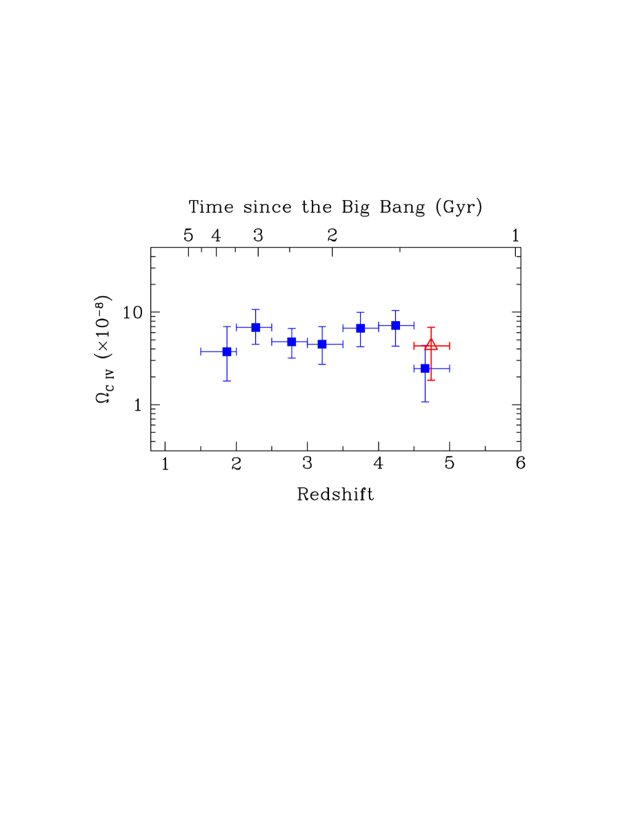
Figure 5: Mass density of C IV, $\Omega_{\rm CIV}$, plotted vs. redshift and cosmic time. For consistency with earlier work, $\Omega_{\rm CIV}$ was calculated from equation (1) and (3) with $\Omega_{\rm M}=1.0$ and $H_{0}=65$  km s^-1 Mpc^-1. (The time scale at the top of the figure, however, refers to the currently favored $\Omega_{\rm M}=0.3$ and $\Omega_{\Lambda}=0.7$ cosmology). Filled squares are the results by Songaila (2001), while the triangle shows the single measurement from the present work. Songaila estimates that at redshifts $z\leq 4$ her data are complete for column densities $\log N$(C IV)$\geq 13$; for a proper comparison with these redshifts we have multiplied our own measurement by a factor of 1.22 which takes into account our incompleteness fraction above $\log N$(C IV)$=13$, as discussed in §5. For clarity, the triangle has been shifted along the $x$-axis by +0.05 from its correct position at $\langle z\rangle=4.688$ (see Table 5). The error bars are 90% confidence limits.

In her analysis, Songaila (2001) divided her sample in bins of $\Delta z=0.5$. The only such bin where we have sufficient statistics to compare with her results is between $z=4.5$ and 5.0, which includes 11 out of the 16 C IV systems detected here. For this subsample of our data, $\Delta X=1.87$, $\langle z\rangle=4.688$ and $\Omega_{\rm CIV}=(3.6\pm 2.1)\times 10^{-8}$. For comparison, Songaila’s (2001) survey in this redshift bin covered $\Delta X=5.36$ at a very similar mean redshift $\langle z\rangle=4.655$, and yielded $\Omega_{\rm CIV}=(2.5^{+1.9}_{-1.4})\times 10^{-8}$ (see Table 5 and Figure 5). Once corrected for incompleteness, we will see below that our estimate of $\Omega_{\rm CIV}$ is $\sim 75$% higher than Songaila’s earlier value, although the two measurements are mutually consistent within the errors.

Our density of absorbers per unit redshift path is two times higher than that of Songaila (2001), presumably reflecting the fact that the high S/N ratios of our spectra allow us to reach further down the column density distribution of C IV. Songaila’s best fit to the $f(N)$ distribution in the redshift range $2.90<z<3.54$ is $f(N)=10^{-12.4}N_{13}^{-1.8}$, where $N_{13}$(C IV) is measured in units of $10^{13}\,$cm^-2. If this relatively steep slope of $f(N)$ persists to the higher redshifts probed here, by integrating over the column density we would expect $f(>N)=5\,N_{13}^{-0.8}$, that is about 5 absorbers with $\log N\geq 13$ per unit absorption distance. Over the redshift interval $z=4.0-5.0$ covered by our spectra, we have identified between 4 and 4.6 systems (depending on whether marginal detections are included or not) with $\log N\geq 13$ per unit $\Delta X$, in very good agreement with the expected value. Thus, within the limited statistics of our sample, it appears that there is little evolution in the density of C IV systems with $\log N{\rm(C~{}IV)}\geq 13.0$.

5 TESTS FOR COMPLETENESS OF C IV DETECTIONS

It is evident from the results in Tables 2, 3, and 4, that our ability to detect C IV absorption systems decreases as $\log N$(C IV) decreases. Most of our systems have $\log N$(C IV) = 13.0–14.0 and only three have $\log N$(C IV) $<13.0$, whereas $f(N)$ still rises at these column densities, at least at $z\simeq 3$ (Ellison et al. 2000). In order to assess the completeness of our sample, we have performed some checks, as follows.

One of us generated a number of fake C IV systems comparable to the number detected in our spectra of SDSS 0231$-$0728 and SDSS 0836$+$0054 (approximately nine systems per simulation). The $b$-values of the fake C IV lines were drawn at random from the observed distribution of $b$-values in our data; similarly their redshifts were chosen randomly from the redshift ranges where we could search for C IV systems. These fake C IV doublets were then added to the real spectra and searched for by one of the two members of our team who had previously identified the real C IV lines. Given the visual, rather than automatic, character of our searches, only a limited number of such trials could be performed. Specifically, we performed three such trials for each of the following values of column density: $\log N$(C IV) =  13.3, 13.5, 13.7, and 14.0 and six trials for $\log N$(C IV) =  13.0 . Thus, the results of these tests are only indicative; they are collected in Table 6.

We found that we could recover essentially all C IV doublets so long as $\log N$(C IV) $\geq 13.3$. Below this value, however, we quickly become incomplete because the equivalent width of the weaker member of the doublet is comparable to residuals from the subtraction of sky emission lines and from the correction for atmospheric absorption, and the chances of blending with these residuals are high. Specifically, we were only able to recover 21 out of 47 fake C IV doublets with $\log N$(C IV) = 13.0. Assuming that this completeness fraction of 45% applies to all systems with $13.0<\log N$(C IV)$<13.3$ in our data, the resulting correction factor to $\Omega_{\rm CIV}$ is +22%. The corresponding correction for systems with $\log N$(C IV)$<13.0$ is more difficult to estimate because our incompleteness becomes severe at these low column densities. If we are 10% complete in the range $12.7<\log N$(C IV)$<13.0$, the corresponding correction to $\Omega_{\rm CIV}$ from this interval alone is +28%; taking both corrections into account would raise the value of $\Omega_{\rm CIV}$ by 50%. More generally, if the steep slope of $f(N)$ found by Songaila (2001) continued below $\log N$(C IV)$=13.0$, we would expect roughly comparable contributions to $\Omega_{\rm CIV}$ from each decade in column density.

Songaila (2001) estimated that at redshifts $z<4$ incompleteness effects become significant in her sample only for column densities $\log N$(C IV)$<13.0$. The simulations described above then suggest that the values of $\Omega_{\rm CIV}$ from our study should be multiplied by a factor of 1.22 for a meaningful comparison with the values at $z<4$. The resulting $\Omega_{\rm CIV}=(4.3\pm 2.5)\times 10^{-8}$ derived here for the interval $z=4.5-5.0$ (where the error does not take into account the uncertainty in the incompleteness correction) can then be seen from Figure 5 to be entirely consistent with the values measured at lower redshifts. Quantitatively, the mean of the five values of $\Omega_{\rm CIV}$ at $z<4$ from the survey by Songaila (2001) is $\langle\Omega_{\rm CIV}\rangle_{1.5<z<4}=5.3\times 10^{-8}$, with a standard deviation $\sigma=1.4\times 10^{-8}$; the value deduced here for $z=4.5-5.0$ is within $1\sigma$ of $\langle\Omega_{\rm CIV}\rangle_{1.5<z<4}$.

6 DISCUSSION

The principal conclusion from this work is that we confirm the findings by Songaila (2001) that the column density distribution $f(N)$ and its integral $\Omega_{\rm C~{}IV}$, which measures the mass density of C IV ions in the intergalactic medium, evidently remain approximately constant over an interval of time which stretches from $\sim 1.25$ to $\sim 4.5$ Gyr after the big bang ($z=5-1.5$).

A straightforward interpretation of these findings is that most of the IGM metals were already in place at the highest currently observable redshifts; it seems unlikely that an invariant distribution could be caused by compensating variations in the metallicity and ionization parameter. In currently popular hierarchical clustering scenarios for the formation of cosmic structures, the assembly of galaxies is a bottom–up process in which large systems result from the merging of smaller subunits. In these theories subgalactic halos with masses comparable to those of present–day dwarf ellipticals form in large numbers at very early times. Their gas condensed rapidly due to atomic line cooling, and became self-gravitating: massive stars formed with some (perhaps top-heavy) initial mass function, synthesized heavy-elements, and exploded as supernovae (SNe) after a few $\times 10^{7}\,$yr, enriching the surrounding medium. It is a simple expectation of the above scenario that the energy deposition by SNe in shallow potential wells will disrupt the newly formed protogalaxies and blow away metal-enriched baryons from the host, causing the pollution of the IGM at early times (e.g. Tegmark, Silk, & Evrard 1993; Gnedin & Ostriker 1997; Madau, Ferrara, & Rees 2001; Mori, Ferrara, & Madau 2002). These subgalactic stellar systems, possibly aided by a population of accreting black holes in their nuclei and/or by an earlier generation of stars in even smaller halos (‘minihalos’ with virial temperatures of only a few hundred kelvins, where collisional excitation of molecular hydrogen is the main coolant), are believed to have generated the ultraviolet radiation and mechanical energy that reheated and reionized the universe (e.g. Haiman & Holder 2003; Loeb & Barkana 2001).

An alternative picture involves later enrichment from Lyman break galaxies (LBGs) instead. In a study which combined QSO absorption line spectroscopy with deep galaxy imaging and spectroscopy in the same fields, Adelberger et al. (2003) have shown that the Lyman $\alpha$ forest and LBGs are more closely related than had been suspected previously. Of particular relevance to the present discussion is the spatial association of strong C IV systems with galaxies: essentially all of the systems with $\log N$(C IV)$\geq 14$ in the Adelberger et al. (2003) sample are found within $\Delta z=600$  km s^-1 and $\Delta r\sim 200h^{-1}$ kpc (proper distance) of a LBG. Adelberger et al. (2003) show that these dimensions, both in space and velocity, are characteristic of the galactic-scale outflows driven by the star formation activity in LBGs. Although the correlation weakens as one moves to lower column densities of C IV, it remains significant over the full range of values of $N$(C IV) sampled here ($\log N{\rm(C~{}IV)}\lower 2.15277pt\hbox{$\;\buildrel>\over{\sim}\;$}13$).

And yet the apparent lack of evolution in $\Omega_{\rm CIV}$ in both scenarios is somewhat puzzling. If these metals are truly intergalactic and due to early pollution, then one might expect the fraction of C which is triply ionized to change between $z=5$ and 1.5, since the physical conditions in the IGM are thought to have evolved between these epochs. Its large scale structure developed dramatically, so that a given optical depth in the Lyman $\alpha$ forest generally refers to condensations of lower overdensity (relative to the mean) at $z=5$ than at $z=1.5$ (e.g. Cen 2003). Perhaps most importantly, the ionizing background may have changed in both intensity and shape, as the comoving density of bright QSOs grew to a peak near $z=2.5$ (Fan et al. 2001a) and if the universe became transparent at wavelengths below 228 Å following the reionization of helium at $z\sim 3$ (Bernardi et al. 2003; Vladilo et al. 2003). Photons with $\lambda<228$ Å have sufficient energy to ionize C³⁺ and thereby reduce the C IV/C_TOT ratio (Davé et al. 1998).

If, on the other hand, the metals are ejected from star-forming LBGs, the abundance and ionization fraction of C atoms are likely to depend more closely on local conditions, rather than those of the IGM at large. As suggested by Adelberger et al. (2003), the approximately constant value of $\Omega_{\rm CIV}$ may then simply mirror the behaviour of the cosmic star formation rate density, which remains essentially flat over the redshift interval $z\simeq 1.5-4$ (Steidel et al. 1999). In this picture, while the mean metallicity of universe grows with cosmic time, one has to assume that this growth is not reflected in the quantity $\Omega_{\rm CIV}$, perhaps because the systems which make the larger contribution to this integral (in current data sets) are associated with outflowing interstellar gas. The true intergalactic metals may be those at the low column density end of $f(N)$, below $\log N$(C IV)$\simeq 13.0$ (Haehnelt 1998), where data are still limited to a few sight-lines to the brightest QSOs (Ellison et al. 2000). Note also that the results of Adelberger et al. apply to galaxies and the IGM at $z=3$, and it remains to be established whether a similar picture holds at higher and lower redshifts. At $z<0.9$ Chen, Lanzetta, & Webb (2001) do find that C IV absorption systems are clustered around galaxies on velocity scales of up to $\sim 250$ km s^-1 and linear scales of up to $\sim 100\,h^{-1}$ kpc, but those systems are generally stronger than the ones considered here.

It is possible that both enrichment mechanisms are at work, and it is also perhaps conceivable that, by coincidence, all complicating effects described above might work in opposite directions and compensate each other to maintain the approximately invariant $\Omega_{\rm CIV}$ found by Songaila (2001) and confirmed here. These possibilities can only be assessed quantitatively with detailed calculations which are beyond the scope of this paper. From an observational point of view, improving the sensitivity of the spectroscopy presented in this paper to include weaker C IV systems is a very challenging task at $z>4$ , even with 8-10 m telescopes. On the other hand, there is an incentive to extend this work to even higher redshifts. Detecting even only the strongest C IV absorbers at $z>5$ (which will require paying special attention to the problem of correcting for atmospheric absorption), would still provide an extremely important probe of the star formation activity at very early epochs.

Support for this work was provided by NSF grant AST-0205738 and by NASA grant NAG5-11513 (P.M.). We are grateful to the ESI team for developing the efficient instrument which made this study possible; to the staff of the Keck Observatory for their competent assistance with the observations; and to Bob Carswell for providing the VPFIT software. We are indebted to Robert Becker, Richard White, and Michael Strauss who kindly contributed most of the ESI exposures of SDSS 1030+0524. We acknowledge valuable discussions with Martin Haehnelt. Max Pettini thanks the Instituto de Astrofísica de Canarias for their hospitality during a visit when this work was completed. Finally, we wish to extend special thanks to those of Hawaiian ancestry on whose sacred mountain we are privileged to be guests. Without their generous hospitality, the observations presented herein would not have been possible.

Table 1: Journal of Observations

QSO	$z_{\rm em}$	$z^{\ast}$	Date	Integration	S/N	$W_{0}$($3\sigma$)
		(mag)		(s)		(mÅ)
SDSS 0231$-$0728	5.421	19.19	2002–Jan–13 &	10 800	50–20	14–35
			2002–Feb–07
SDSS 0836+0054	5.803	18.74	2002–Jan–13 &	32 400	80–40	8–17
			2002–Feb–07
SDSS 1030+0524	6.305	20.05	2002–Jan–10,11,12	28 500	60–15	11–45

Table 2: C IV Absorption Systems in SDSS 0231$-$0728

Number	$z_{\rm abs}$	$b$	$\log N{\rm(C~{}IV)}$	Comments
		(km s-1)
1	$4.1242\pm 0.0001$	$57\pm 13$	$13.03\pm 0.05$
2	$4.13921\pm 0.00002$	$13\pm 4$	$13.19\pm 0.02$
3	$4.22641\pm 0.00009$	$40\pm 9$	$13.16\pm 0.06$
4	$4.2991\pm 0.0001$	$45\pm 12$	$13.34\pm 0.07$
5	$4.5070\pm 0.0001$	…	$12.75:$	Marginal
6	$4.54420\pm 0.00008$	$35\pm 8$	$13.18\pm 0.05$
7	$4.5701\pm 0.0001$	$58\pm 13$	$13.38\pm 0.06$
8	$4.7556\pm 0.0001$	$53\pm 12$	$13.35\pm 0.07$	Marginal

Table 3: C IV Absorption Systems in SDSS 0836+0054

Number	$z_{\rm abs}$	$b$	$\log N{\rm(C~{}IV)}$	Comments
		(km s-1)
1	$4.49951\pm 0.00009$	$15:$	$12.50\pm 0.08$
2	$4.51440\pm 0.00003$	$41\pm 2$	$13.52\pm 0.02$
3	$4.61237:$	…	$12.7:$	Marginal
4	$4.66874\pm 0.00005$	…	$>13.04$	Lines are saturated
5a	$4.6826\pm 0.0002$	$71\pm 15$	$13.52\pm 0.07$	Poor fit
5b	$4.68487\pm 0.00007$	$39\pm 8$	$13.57\pm 0.07$	Poor fit
5c	$4.68690\pm 0.00004$	$35\pm 4$	$13.68\pm 0.03$	Poor fit
6	$4.7739\pm 0.0001$	$65\pm 10$	$13.15\pm 0.05$	Marginal
7	$4.99695\pm 0.00005$	$36\pm 4$	$13.56\pm 0.03$

Table 4: C IV Absorption System in SDSS 1030$+$0524

Number	$z_{\rm abs}$	$b$	$\log N{\rm(C~{}IV)}$	Comments
		(km s-1)
1	$4.94866\pm 0.00006$	$58\pm 4$	$13.98\pm 0.02$

Table 5: Statistics of C IV Absorption

Sample	$z_{\rm abs}$	$\Delta X$	$\langle z_{\rm abs}\rangle$	Number of	$\Omega_{\rm CIV}$
				Lines	($\times 10^{-8}$)
Whole sample	4.0–5.0	3.29	4.568	16	$2.4\pm 1.2$
Subsample	4.5–5.0	1.87	4.688	11	$3.6\pm 2.1$
Songaila (2001)	4.5–5.0	5.36	4.655	16	$2.5^{+1.9}_{-1.4}$

Table 6: Incompleteness Corrections

$\log N$(C IV)	Fraction of C IV Systems	Correction Factor
	Detected	to $\Omega_{\rm CIV}$
14.0	1.0	1.0
13.7	1.0	1.0
13.5	1.0	1.0
13.3	0.96	1.01
13.0	0.45	1.22

Figure 3: Normalised absorption profiles (histograms) of C IV systems in SDSS 0836+0054. The $y$-axis is residual intensity, while the $x$-axis gives the observed wavelength in Å. The thin continuous lines show theoretical profiles produced by VPFIT with the parameters listed in Table 3. Vertical tick marks indicate the positions of the C IV $\lambda\lambda 1548.2041,1550.7812$ doublet lines. The line near the zero level shows the $1\sigma$ error spectrum. The weak C IV system at $z_{\rm abs}=4.49951$ (top left-hand panel) is shown for clarity on an expanded $y$-scale; in this case the error spectrum has been offset by $+0.6$ in $y$.

References

- (1)
- (2) Adelberger, K. L., Steidel, C. C., Shapley, A. E., & Pettini, M. 2003, ApJ, 584, 45
- (3)
- (4) Anderson, S. F. et al. 2001, AJ, 122, 503
- (5)
- (6) Becker, R. H. et al. 2001, AJ, 122, 2850
- (7)
- (8) Bernardi, M. et al. 2003, AJ, 125, 32
- (9)
- (10) Cen, R. 2003, http://astro.Princeton.EDU/~cen/PROJECTS/p2/p2.html
- (11)
- (12) Cen, R. & McDonald, P. 2002, ApJ, 570, 457
- (13)
- (14) Chen, H. W., Lanzetta, K. M., & Webb, J. K. 2001, ApJ, 556, 158
- (15)
- (16) Davé, R., Hellsten, U., Hernquist, L., Katz, N., & Weinberg, D. H. 1998, ApJ, 509, 661
- (17)
- (18) Efron, B., & Tibshirani, R.J. 1993, An Introduction to the Bootstrap (New York: Chapman & Hall)
- (19)
- (20) Ellison, S. L., Songaila, A., Schaye, J., & Pettini, M. 2000, AJ, 120, 1175
- (21)
- (22) Fan, X. et al. 2001a, AJ, 121, 54
- (23)
- (24) Fan, X., et al. 2001b, AJ, 122, 2833
- (25)
- (26) Fan, X., et al. 2003, AJ, 125, 1649
- (27)
- (28) Fan, X., Narayanan, V. K., Strauss, M. A., White, R. L., Becker, R. H., Pentericci, L., & Rix, H.-W. 2002, AJ, 123, 1247
- (29)
- (30) Gnedin, N. Y., & Ostriker, J. P. 1997, ApJ, 486, 581
- (31)
- (32) Haehnelt M. G. 1998, The Young Universe: Galaxy Formation and Evolution at Intermediate and High Redshift, ASP Conf. Ser. 146, 249
- (33)
- (34) Haiman, Z., & Holder, G. P. 2003, ApJ, submitted (astro-ph/0302403)
- (35)
- (36) Hu, E. M., Cowie, L. L., McMahon, R. G., Capak, P., Iwamuro, F., Kneib, J.-P., Maihara, T., & Motohara, K. 2002, ApJ, 568, L75
- (37)
- (38) Kodaira, K. et al. 2003, PASJ, in press (astro-ph/0301096)
- (39)
- (40) Kogut, A., et al. 2003, ApJ, submitted (astro-ph/0302213)
- (41)
- (42) Lanzetta, K. M. 1993, ASSL Vol. 188: The Environment and Evolution of Galaxies, 237
- (43)
- (44) Lehnert, M. D., & Bremer, M. 2003, ApJ, in press (astro-ph/0212431)
- (45)
- (46) Loeb, A., & Barkana, R. 2001, ARA&A, 39, 19
- (47)
- (48) Madau, P., Ferrara, A., & Rees, M. J. 2001, ApJ, 555, 92
- (49)
- (50) Massey, P. & Gronwall, C. 1990, ApJ, 358, 344
- (51)
- (52) Massey, P., Strobel, K., Barnes, J. V., & Anderson, E. 1988, ApJ, 328, 315
- (53)
- (54) Mori, M., Ferrara, A., & Madau, P. 2002, ApJ, 571, 40
- (55)
- (56) Morton, D.C. 2003, ApJS, in press (http://www.hia-iha.nrc-cnrc.gc.ca/staff/morton_e.html)
- (57)
- (58) Nachman, P., & Hobbs, L.M. 1973, ApJ, 182, 481
- (59)
- (60) Rauch, M., Sargent, W. L. W., Womble, D. S., & Barlow, T. A. 1996, ApJ, 467, L5
- (61)
- (62) Sheinis, A. I., Miller, J. S., Bolte, M., & Sutin, B. M. 2000, Proc. SPIE, 4008, 52
- (63)
- (64) Songaila, A. 2001, ApJ, 561, L153
- (65)
- (66) Spergel, D.N., et al. 2003, ApJ, submitted (astro-ph/0302207)
- (67)
- (68) Stanway, E. R., Bunker, A. J., & McMahon, R. G. 2003, MNRAS, in press (astro-ph/0302212)
- (69)
- (70) Steidel, C. C., Adelberger, K. L., Giavalisco, M., Dickinson, M., & Pettini, M. 1999, ApJ, 519, 1
- (71)
- (72) Storrie-Lombardi, L., McMahon, R. G., & Irwin, M. 1996, MNRAS, 283, 79P
- (73)
- (74) Tegmark, M., Silk, J., & Evrard, A. 1993, ApJ, 417, 54
- (75)
- (76) Tytler, D. 1987, ApJ, 321, 49
- (77)
- (78) Vladilo, G., Centurión, M., D’Odorico, V., & Péroux, C. 2003, A&A, 402, 487
- (79)
- (80) White, R. L., Becker, R. H., Fan, X., & Strauss, M.A. 2003, AJ, submitted (astro-ph/0303476)
- (81)
- (82) Yan, H., Windhorst, R. A., & Cohen, S. H. 2003, ApJ, 585, L93
- (83)