The WSRT wide-field H i survey

We have used the Westerbork array to carry out an unbiased wide-field survey for H i emission features, achieving an rms sensitivity of about 18 mJy/Beam at a velocity resolution of 17 km s^-1 over 1800 deg² and between $-1000\leavevmode\nobreak\ <\leavevmode\nobreak\$V${}_{Hel}\leavevmode\nobreak\ <\leavevmode\nobreak\ +6500$ km s^-1. The primary data consists of auto-correlation spectra with an effective angular resolution of 49^′ FWHM, although cross-correlation data were also acquired. The survey region is centered approximately on the position of Messier 31 and is Nyquist-sampled over 60$\times$30^∘ in R.A.$\times$Dec. More than 100 distinct features are detected at high significance in each of the two velocity regimes (negative and positive LGSR velocities). In this paper we present the results for our H i detections of external galaxies at positive LGSR velocity. We detect 155 external galaxies in excess of 8$\sigma$ in integrated H i flux density. Plausible optical associations are found within a 30^′ search radius for all but one of our H i detections in DSS images, although several are not previously cataloged or do not have published red-shift determinations. Our detection without a DSS association is at low galactic latitude. Twenty-three of our objects are detected in H i for the first time. We classify almost half of our detections as “confused”, since one or more companions is cataloged within a radius of 30^′ and a velocity interval of 400 km s^-1. We identify a handful of instances of significant positional offsets exceeding 10 kpc of unconfused optical galaxies with the associated H i centroid, possibly indicative of severe tidal distortions or uncataloged gas-rich companions. A possible trend is found for an excess of detected H i flux in unconfused galaxies within our large survey beam relative to that detected previously in smaller telescope beams, both as function of increasing distance and increasing gas mass. This may be an indication for a diffuse gaseous component on 100 kpc scales in the environment of massive galaxies or a population of uncataloged low mass companions. We use our galaxy sample to estimate the H i mass function from our survey volume. Good agreement is found with the HIPASS BGC results, but only after explicit correction for galaxy density variations with distance.

1 Introduction

Unbiased wide-field surveys are an indispensible means for determining the physical content of our extended environment. The SDSS (Sloan Digital Sky Survey (York et al. york00 (2000))) is a prime example of the way in which such work is providing new insights at optical wavelengths into both the nearby and distant universe. At radio frequencies there have been a number of wide-field surveys for both continuum sources and, to a lesser extent, emitters and absorbers in specific spectral lines. The HIPASS survey (Barnes et al. barn01 (2001)) marks an important milestone in achieving high sensitivity to H i emission over more than half of the sky (given it’s ongoing extension of the Declination coverage from 0 to +25^∘). HIPASS has provided a deep inventory of both negative and positive LGSR (Local Group Standard of Rest) velocity H i emission features. The negative velocity features (Putman et al. putm02 (2002)) are primarily associated in some way with the Galaxy and other Local Group objects, while the positive velocity features are primarily associated with moderately nearby ($<$ 100 Mpc) external galaxies (eg. Kilborn et al. kilb02 (2002)). A northern hemisphere counterpart to the HIPASS survey is now underway in the form of HIJASS (H i Jodrell All Sky Survey, Lang et al. lang03 (2003)).

An interesting component of the negative velocity H i sky are the so-called compact high velocity clouds, CHVCs (Braun & Burton brau99 (1999)), which are isolated in position and velocity from the more extended high velocity H i complexes down to column densities below about $N_{\rm HI}$ = 1.5$\times 10^{18}$cm^-2. The suggestion has been made that these objects may be the most distant component of the high velocity cloud phenomenon, perhaps extending to 100’s of kpc from their host galaxies. A critical prediction of this scenario (De Heij et al. dehe02 (2002)) is that a large population of faint CHVCs should be detected in the vicinity of M31 (at declination +40^∘) if enough sensitivity were available. While current observational data are consistent with this scenario, they are severely limited by the modest point source sensitivity available at northern declinations (within the Leiden/Dwingeloo Survey (Hartmann & Burton hart97 (1997))) which is almost an order of magnitude poorer than that of HIPASS in the south.

We have undertaken a moderately sensitive large-area H i survey both to test for the predicted population of faint CHVCs near M31 as well as to carry out an unbiased search for H i emission associated with background galaxies. We have achieved an rms sensitivity of about 18 mJy/Beam at a velocity resolution of 17 km s^-1 over 1800 deg² and between $-1000\leavevmode\nobreak\ <\leavevmode\nobreak\$V${}_{Hel}\leavevmode\nobreak\ <\leavevmode\nobreak\ +6500$ km s^-1. The corresponding rms column density sensitivity for emission filling the 3000$\times$2800 arcsec effective beam area is about 4$\times 10^{16}$cm^-2 over 17 km s^-1. For comparison, the HIPASS survey has achieved an rms of about 14 mJy/Beam at a velocity resolution of 18 km s^-1, yielding a slightly superior flux sensitivity. On the other hand, the column density sensitivity for emission filling our larger beam exceeds that of HIPASS by almost an order of magnitude. Since the linear FWHM diameter of our survey beam varies from about 10 kpc at a distance of 0.7 Mpc to more than 1 Mpc at 75 Mpc, it is only at Local Group distances that the condition of beam filling is likely to be achieved. Compared to the Leiden/Dwingeloo Survey, we achieve an order of magnitude improvement in both flux density and brightness sensitivity. We detect more than 100 distinct features at high significance in each of the two velocity regimes (negative and positive LGSR velocities). In this paper we will describe the survey observations and data reduction procedures in § 2, followed by a presentation of the results for our H i detections of external galaxies in § 3 and closing with a brief discussion of these results in § 4. Our results at negative LGSR velocities will be presented in a companion paper.

2 Observations and Data Reduction

2.1 Survey Strategy

Our survey area was defined to have an extent of 60$\times$30 true degrees oriented in $\alpha_{2000}\times\delta_{2000}$ and centered on ($\alpha_{2000},\delta_{2000}$) = (10^∘,35^∘), about 5^∘south of the M31 nuclear position. Data were acquired in a drift-scan mode, whereby the 25 m telescopes of the WSRT array were kept stationary at a specified start position and the sky drifted past at the earth-rotation rate. Each telescope beamwidth is about 35 arcmin FWHM at an observing frequency of 1410 MHz. The fourteeen telescopes of the array were split into two sub-arrays of seven telescopes each. The two sub-arrays were pointed at declinations offset from one another by 15 arcmin, in order to achieve Nyquist-sampled declination coverage of the survey area in half the time that would otherwise be required. The recorded data were averaged over 60 sec, corresponding to an angular drift of about 15 arcmin of right ascension, to yield Nyquist-sampling in the scan direction of the telescope beam.

Although the primary objective of the survey was acquisition of auto-correlation data, it was also desirable to acquire cross-correlation data simultaneously for the two sub-arrays of seven telescopes which observed the same set of positions on the sky. To this end, electronic tracking was employed during each 60 second integration directed at the sequence of central positions that was sweeping through the telescope beam at the earth-rotation rate. The two sub-arrays were each composed of six telescopes with short relative spacings (betweem 36 and 144 m) and a seventh telescope at a larger separation (of about 1.5 km). The duration of the drift-scan observations varied with declination from about 4.3 to 6.2 hours. A typical observing sequence consisted of a standard observation of a primary calibration source (3C48 or 3C286), a dual sub-array drift-scan observation and in some cases a second dual sub-array drift-scan observation. Each such session provided the survey data for a strip of either 60$\times$0.5 or 60$\times$1 true degrees. Thirty of the “double” sessions, lasting some 320 hours, could in principle provide the complete survey coverage.

In practise, the observations were distributed over some 52 sessions in the period 2002/09/04 to 2002/11/16. An effort was made to acquire the drift-scan data only after local sunset and before local sunrise to minimize solar interference. This was largely successful, with only a few hours of data showing the effects of the sun above the horizon. An effort was also made to insure that the drift-scan data was only acquired at moderately high elevations, both to eliminate the possibility of inter-telescope shadowing and to optimize the system temperature. Essentially all observations were done at elevations between 45 and 85 deg, for which the system temperature variations are observed to be less than 1 K, corresponding to about 3%. Repeat coverage of a number of scans was obtained in cases where instrumental failure or severe interference led to a significant increase in the noise level.

Data was acquired in two 20 MHz IF bands centered at 1416 and 1398 MHz. The 18 MHz spacing of the two bands was chosen to provide a contiguous velocity coverage at a uniform nominal sensitivity. All auto- and cross-correlations were recorded for both linear polarizations in 512 uniformly weighted spectral channels across each 20 MHz band. A hanning smoothing was applied after the fact to minimize the spectral side-lobes of interference, yielding a spectral resolution of 78.125 kHz, corresponding to about 16.6 and 16.8 km s^-1  in the two bands.

2.2 Data Reduction

The drift-scan data for each sub-array was inspected and flagged in Classic AIPS using the SPFLG utility. Any questionable features appearing in the (time,frequency) display of each auto-correlation baseline were critically compared amongst the 14 independent estimates (7 telescopes and 2 polarizations) that were available. Any features which were not reproduced in the other simultaneous spectra (from telescopes seperated by as much as 2 km) were flagged. This allowed quite effective discrimination against interference.

Absolute flux calibration of both the auto- and cross-correlation data was provided by the observed mean cross-correlation coefficient measured for the standard calibration sources (3C48 or 3C286) of known flux density. The measured ratio of flux density to correlation coefficient averaged over all 14 telescopes and 2 polarizations was 300$\pm$10 Jy/Beam. Although there are variations (typically less than about 10%) amongst the 28 independent receiver systems, the average gain of the system (at this frequency) has remained constant at the quoted value over a period of several years to better than 5 percent. The calibrator observation of each observing session was used both to determine the average gain value appropriate for the auto-correlations as well as providing phase and gain solutions appropriate for the calibration of the cross-correlation drift-scan data in that session.

Two different methods were employed to generate data-cubes of the auto-correlation data. The first method employed a local robust average of a 30 minute sliding window to estimate the band-pass as a function of time and a 850 km s^-1 sliding window to estimate the continuum level as a function of frequency. Only those values between the first and third quartiles were included in these averages, making them moderately robust to outliers, including H i emission features, in the data. This method could be applied blindly and produced the most uniform noise characteristics in the resulting cube. As such, it was well-suited for the automated detection of faint sources. However, moderately bright sources of H i emission that were extended either spatially or in velocity produced localized negative artifacts. The best results under these circumstances were obtained with the more complicated procedure outlined below: 1) a quadratic baseline in time was fit to the entire drift-scan (of 4 to 6 hour duration) and divided out after masking out any localized regions of emission, 2) a constant offset was determined and divided out of each frequency spectrum after masking out any regions of line emission (including the extended emission from the Galaxy), 3) a quadratic baseline in frequency was fit and subtracted from the lower half (the first 10 MHz) of each frequency spectrum after masking out any regions of line emission, 4) an alternative baseline solution (primarily for the upper 10 MHz of each band) was derived from a boxcar smoothed spectrum with 6 MHz box-width and subtracted from each frequency spectrum after masking out any regions of line emission, 5) a cubic baseline in time was fit and subtracted out of each drift-scan after masking out any localized regions of emission, 6) all unflagged data for each position and frequency were averaged, 7) the entire process (steps (1) through (6) above) was repeated using an updated mask to isolate regions of significant emission from the baseline determination.

The rationale for each step noted above was the folowing; step (1) was intended to compensate for long timescale variations in the basic bandpass shape, step (2) for the possible contributions of bright continuum sources to the system temperature as function of time, steps (3) and (4) for residual corrections to the bandpass shape on short timescales (where it was found empirically that the two different methods gave somewhat superior results in the two halves of the band) and step (5) for residual corrections to the bandpass shape on intermediate timescales.

Although the survey strategy was designed to provide the most stable possible bandpass response, this proved to be somewhat disappointing. During the course of the observing campaign it was established that there were systematic variations in the bandpass shape at the level of about 1:1000 which were closely correlated with small variations in ambient temperature in the vicinity of the IF system electronics on timescales of 0.5 to 5 hours. Steps were taken to stabilize the airflow and ambient temperature which led to a substantial improvement in baseline stability. Even so, the remaining fluctuations are still a limiting factor to the final auto-correlation sensitivity, at least in the upper one third of each 20 MHz band, where they were most severe.

The drift-scan data were resampled in frequency to convert from the fixed geocentric frequencies of each observing date to heliocentric radial velocities at each observed position. A Gaussian smoothing with 1800 true arcsec FWHM was applied in RA before combining the 120 drift-scans into a data-cube for each 20 MHz band. A spatial resampling was then carried out to convert from the rectangular ($\alpha,\delta$) of the acquired data to a projected ($\alpha,\delta$) geometry. Finally, a spatial convolution with a 1800$\times$900 arcsec FWHM Gaussian with PA = 0^∘was applied to introduce the desired degree of spatial correlation in the result.

The average primary beam of the WSRT array at an observing frequency of 1400 MHz has been determined with a holographic measurement (and can be found depicted at http://www.astron.nl/wsrt/wsrtGuide/WSRT21BEAM.PS). The central positive lobe has an area of 1535 arcmin² and is moderately well-fit by a Gaussian with 2235 arcsec FWHM. Peak sidelobe levels are about 0.1%. The same sequence of spatial smoothings described above, first a 900” box-car in RA to simulate the drift-scan, then a 1800” Gaussian in RA and then a 900$\times$1800” Gaussian in ($\alpha,\delta$) was applied to a digital representation of the primary beam. This allowed estimation of the effective beam size for the survey, which can be approximated by a Gaussian of 3020$\times$2810 arcsec at PA = 90^∘, as well as the beam dilution factor needed to preserve the absolute flux scale in units of Jy/Beam.

Figure 1: Variation of rms fluctuation level with heliocentric velocity over the survey velocity coverage.

The resulting rms fluctuation level as function of heliocentric velocity is shown in Fig. 1 as determined from a fit to the peak of the histogram in each velocity channel. The effective velocity coverage extends from about $-1000\leavevmode\nobreak\ <\leavevmode\nobreak\$V${}_{Hel}\leavevmode\nobreak\ <$ 6500 km s^-1. An increased noise level is seen for $-200\leavevmode\nobreak\ <\leavevmode\nobreak\$V${}_{Hel}\leavevmode\nobreak\ <$150 km s^-1 due to intermediate velocity emission features associated with the Galaxy. Slightly elevated noise levels are also seen for $1700\leavevmode\nobreak\ <\leavevmode\nobreak\$V${}_{Hel}\leavevmode\nobreak\ <$ 2600 km s^-1 and $5500\leavevmode\nobreak\ <\leavevmode\nobreak\$V${}_{Hel}\leavevmode\nobreak\ <$ 6500 km s^-1 due to the problems of spectral baseline stability in the upper third of each 20 MHz band as noted above. A small velocity range near 1500 km s^-1 also has a slightly higher noise due to a significant degree of data flagging at this velocity that was made necessary by recurring interference.

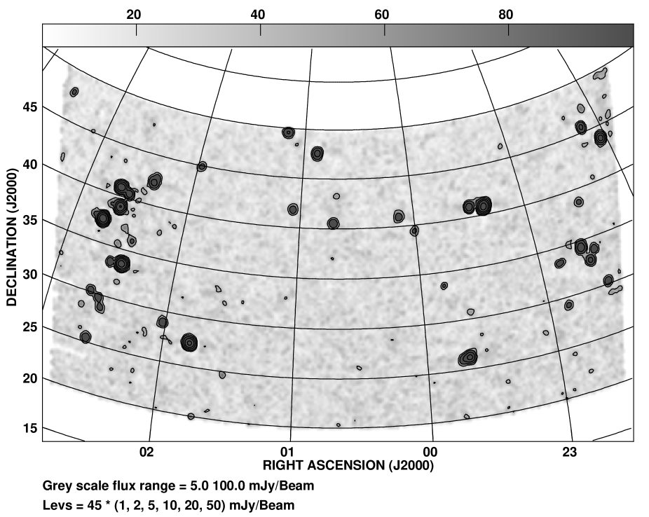
Figure 2: Illustration of the survey sky coverage and galaxy detections between $250\leavevmode\nobreak\ <\leavevmode\nobreak\$V${}_{Hel}\leavevmode\nobreak\ <1500$ km s^-1. The peak brightness of H i emission at a velocity resolution of 42 km s^-1  FWHM is shown in this velocity interval with a linear greyscale between and 5 and 100 mJy/Beam and contours drawn at (1, 2, 5, 10, 20 and 50) times 45 mJy/Beam.

3 Results

An overview of the survey sky coverage, together with an indication of some of the galaxy detections, is given in Fig. 2. Peak H i brightness at a velocity resolution of 42 km s^-1  FWHM is shown in the figure for the velocity interval $250\leavevmode\nobreak\ <\leavevmode\nobreak\$V${}_{Hel}\leavevmode\nobreak\ <1500$ km s^-1. The first contour in the figure corresponds to approximately 4$\sigma$ at this velocity resolution. The total solid angle observed is 1800 deg². The rms fluctuation level varies slightly with recession velocity (as shown in Fig. 1). The positions of bright continuum sources (brighter than a few Jy) display residual fluctuations in excess of the nominal noise level. The resulting noise distribution is not entirely Gaussian, and for this reason we consider it necessary to adopt a conservative cut-off in our blind extraction of reliable H i detections. Rosenberg & Schneider (rose02 (2002)) have shown from their extensive simulations involving insertion of artificial sources into surveys of this type that an asymptotic completeness level is reached at a signal-to-noise ratio of about 8 (in terms of integrated signal strength relative to the error in the integral), while below this signal-to-noise ratio the completeness drops dramatically.

Candidate H i detections in our combined data-cubes were determined by two different methods. In the first instance, the SAD source finding algorithm within Classic AIPS was used to extract all local peaks in excess of 3 times the local RMS level in datacubes having Nyquist-sampled velocity resolutions of 2, 5, 10, 20 and 50 times the basic velocity channel seperation of 8.4 km s^-1. A reduced list of emission candidates having a detected peak in excess of 5$\sigma$ in at least two different velocity channels or two different velocity smoothings was extracted for further analysis. The aim of this procedure was to reliably recover significant detections spanning a wide range in observed linewidth. A complimentary list of candidates was determined from visual inspection of subsequent channel maps as well as subsequent postion–velocity projections using the KVIEW display program (Gooch gooc95 (1995)) for the data-cubes at velocity resolutions of 2, 5, 10, 20 and 50 times the basic velocity channel seperation of 8.4 km s^-1. Candidate features were rejected if their response in our data-cubes before spatial smoothing were inconsistent with the telescope beam response in either $\alpha$ or $\delta$, implying the time variable signature of interference. The properties of some 500 candidate detections were then estimated in detail. In particular, the integrated line strength was determined for each candidate by extracting the single spectrum from our spatially smoothed data-cubes with the highest total flux density. The underlying assumption is that essentially all galaxies will be unresolved with our effective FWHM beamsize of 3020$\times$2810 arcsec, corresponding to 73$\times$68 kpc at the nearest galaxy distance of 5 Mpc. This assumption was tested by comparing the peak with the integrated flux of a Gaussian fit to an image of integrated H i for each source. While some sources show clear signs of confusion from nearby companions (which will be discussed in detail below), there were no instances of our having significantly resolved single galaxies with our survey beam. The associated error in flux density was determined over a velocity interval of 1.5$\times$W₂₀ (where W₂₀ is the velocity width of the emission profile at 20% of the peak intensity) together with the actual rms fluctuation level associated with this velocity interval.

Only the 155 candidates with an integrated flux density exceeding 8 times the associated error where retained. Spectra of each detection are shown in Fig. 3 for the single spatial pixel with the maximum integrated H i signal. The source centroid positions were determined from either a Gaussian or a parabolic fit to the peak in images of integrated H i line strength over the full velocity extent of each detection. The positional accuracy is dependent on the signal-to-noise ratio, and is expected to be roughly HWHM/(s/n), implying about 3 arcmin rms in both $\alpha$ and $\delta$ for the lowest significance detections.

Figure 3: H i spectra of detected galaxies. The complete set of panels for all detected galaxies is only available in the electronic version of the paper at http://www.epdsciences.org. The catalog designation is indicated in the upper left of each panel, while the likely optical ID is indicated in the upper right.

Table 1: Properties of H i detected Galaxies

Name	R.A. (J2000)	Dec. (J2000)	VHel	W20	Sint	$\delta$Sint	log(MHI)	Optical ID	Notea	Offset	Comp.b
	$\rm(h\ m\ s)$	$\rm(^{\circ}\ {}^{\prime}\ {}^{\prime\prime})$	(km s-1)		(Jy km s-1)		(M⊙)			(’)
(1)	(2)	(3)	(4)	(5)	(6)	(7)	(8)	(9)	(10)	(11)	(12)
J2158+4219	21 58 47	42 19 46	4335	245	9:	–	9.92	UGC 11864		9.8	004
J2202+4838	22 02 49	48 38 16	3605	300	9.3	0.82	9.77	—??—-		0.0	000
J2203+4345	22 03 36	43 45 24	455	165	99.5	0.64	9.37	UGC 11891		0.7	008
J2206+4714	22 06 23	47 14 05	1110	240	34.4	0.77	9.45	UGC 11909		1.5	004
J2208+4433	22 08 54	44 33 50	3110	230	24.3	0.72	10.07	UGC 11923	c	1.5	108
J2209+3917	22 09 22	39 17 30	4710	125	7.1	0.55	9.87	UGC 11929	c	3.0	100
J2210+4101	22 10 10	41 01 03	4600	350	59.6	0.90	10.78	NGC 7223	c	0.2	326
J2212+4521	22 12 38	45 21 55	1100	200	46.9	0.67	9.58	NGC 7231	c	2.6	308
J2216+4122	22 16 55	41 22 33	4190	490	17.9	1.00	10.18	UGC 11973	c	7.7	102
J2217+4542	22 17 26	45 42 25	5730	120	8.8	0.55	10.13	UGC 11979		7.6	006
J2218+4029	22 18 05	40 29 17	1198	90	5.4	0.40	8.70	NGC 7250		5.1	002
J2228+2907	22 28 12	29 07 10	990	220	14.6	0.72	8.99	NGC 7286		4.9	005
J2228+3016	22 28 22	30 16 10	985	85	18.5	0.44	9.09	NGC 7292		1.6	002
J2230+3842	22 30 33	38 42 50	695	55	9.6	0.33	8.59	KKR 71		1.5	005
J2230+3344	22 30 44	33 44 55	890	120	28.6	0.52	9.22	UGC 12060		1.9	003
J2233+3903	22 33 14	39 03 31	5385	410	21.7	1.01	10.47	UGC 12077	c	7.1	135
J2234+3251	22 34 13	32 51 09	805	95	26.8	0.46	9.12	UGC 12082		0.7	000
J2237+3424	22 37 01	34 24 32	835	510	230.5	1.13	10.08	NGC 7331		0.8	006
J2237+2353	22 37 25	23 53 23	1378	372	8.9	0.57	9.00	NGC 7332	c	5.5	204
J2242+3744	22 42 19	37 44 41	4695	275	10.8	0.82	10.05	CGCG 514-098		6.1	004
J2250+2909	22 50 23	29 09 55	895	120	16.3	0.52	8.97	UGC 12212		2.3	000
J2304+2708	23 04 17	27 08 25	1060	150	6.6	0.53	8.68	UGC 12340		3.9	009
J2313+2900	23 13 32	29 00 04	3690	220	17.1	0.70	10.05	UGC 12430	c	2.5	103
J2322+4050	23 22 05	40 50 03	380	255	342.0	0.81	9.79	NGC 7640	o	0.7	001
J2326+2504	23 26 45	25 04 20	3490	370	21.3	0.91	10.10	NGC 7664		1.3	005
J2326+3046	23 26 50	30 46 06	4520	140	5.3	0.53	9.70	UGC 12609	+	21.2	001
J2327+2334	23 27 35	23 34 19	3440	240	14.5	0.73	9.92	NGC 7673	c	1.8	103
J2328+2234	23 28 54	22 34 46	3475	350	10.8	0.95	9.80	NGC 7678		11.2	013
J2329+4101	23 29 55	41 01 20	425	135	75.6	0.55	9.19	UGC 12632	o	2.0	001
J2330+3008	23 30 45	30 08 45	4530	160	11.7	0.59	10.05	UGC 12639		6.0	002
J2331+2851	23 31 31	28 51 40	5510	240	8.1	0.70	10.05	Mrk 0930	c	7.9	104
J2333+2657	23 33 20	26 57 10	3695	145	6.9	0.56	9.65	CGCG 476-066		5.2	006
J2336+3216	23 36 09	32 16 26	4955	320	12.1	0.80	10.14	UGC 12693	c	8.6	101
J2337+3602	23 37 32	36 02 57	5020	700	27.0	1.20	10.50	UGC 12697	++	19.6	001
J2337+3048	23 37 39	30 48 40	295	165	9.3	0.66	8.07	UGC 12713		9.8	002
J2339+2509	23 39 44	25 09 31	4935	75	3.6	0.43	9.61	CGCG 476-100	?	4.0	008
J2340+2615	23 40 43	26 15 44	750	140	89.1	0.56	9.56	UGC 12732	o	1.7	009
J2346+3330	23 46 15	33 30 34	4950	370	11.8	0.96	10.13	UGC 12776		8.4	004
J2347+2932	23 47 29	29 32 59	5115	525	19.1	1.14	10.36	NGC 7753	c	6.6	100
J2348+2612	23 48 58	26 12 45	800	100	18.8	0.47	8.93	UGC 12791		2.0	004
J2349+4755	23 49 12	47 55 30	4620	165	6.1	0.64	9.79	UGC 12796		1.3	000
J2356+3203	23 56 05	32 03 29	4850	265	11.2	0.73	10.09	UGC 12845		10.7	009
J2358+4656	23 58 58	46 56 57	5080	430	10.8	1.06	10.11	IC 1525	c	4.7	303
J0000+3927	00 00 22	39 27 20	330	70	7.5	0.43	8.03	UGC 12894		2.4	000
J0000+2320	00 00 37	23 20 27	4560	85	5.4	0.41	9.71	UGC 12914	c	16.4	102
J0003+3132	00 03 27	31 32 25	4940	390	11.0	0.98	10.09	CGCG 498-067	c	8.5	606
J0004+3129	00 04 20	31 29 32	5020	150	8.8	0.41	10.01	NGC 7819	c	1.5	304
J0006+4749	00 06 55	47 49 15	4300	85	10.3	0.44	9.95	UGC 00048		4.6	002
J0007+2740	00 07 27	27 40 17	4620	190	15.1	0.62	10.17	NGC 0001	c	3.3	129
J0007+4056	00 07 48	40 56 23	305	90	16.0	0.47	8.32	UGC 00064		3.9	002
J0010+2557	00 10 07	25 57 06	4618	360	22.9	0.97	10.35	NGC 0023	c	3.4	202
J0011+3319	00 11 03	33 19 27	4806	370	18.6	0.86	10.30	NGC 0021	c	3.8	409

• Explanation of notes: “c” for confused sources, “?” for sources without a previous red-shift ,“o” for cases of a significant centroid offset of less than 10 kpc, “+” for cases of centroid offset in excess of 10 kpc and $>5\sigma$, “++” for centroid offset greater than 10 kpc and $>10\sigma$.

• A three digit “confusion” index, “abc” enumerating the number of cataloged campanions (truncated at 9) within a 30^′ radius which are (a) within 400 km s^-1, (b) between 400 and 1000 km s^-1and (c) of unknown red-shift.

Table 2: Properties of H i detected Galaxies (continued.)

Name	R.A. (J2000)	Dec. (J2000)	VHel	W20	Sint	$\delta$Sint	log(MHI)	Optical ID	Notea	Offset	Comp.b
	$\rm(h\ m\ s)$	$\rm(^{\circ}\ {}^{\prime}\ {}^{\prime\prime})$	(km s-1)		(Jy km s-1)		(M⊙)			(’)
(1)	(2)	(3)	(4)	(5)	(6)	(7)	(8)	(9)	(10)	(11)	(12)
J0012+4147	00 12 16	41 47 48	5000	100	5.0	0.45	9.76	UGC 00112		2.9	001
J0013+2655	00 13 51	26 55 49	4680	244	12.2	0.78	10.09	UGC 00127		2.5	001
J0013+3606	00 13 58	36 06 18	4580	120	7.0	0.49	9.83	UGC 00128		6.8	003
J0028+4320	00 28 59	43 20 55	190	40	4.1	0.34	7.52	UGC 00288		5.0	003
J0042+4031	00 42 31	40 31 36	230	100	22.4	0.50	8.31	And IV		2.7	019
J0043+2705	00 43 58	27 05 05	5190	240	14.8	0.79	10.26	UGC 00470	c	14.7	102
J0047+2951	00 47 52	29 51 32	5030	105	3.9	0.46	9.65	CGCG 501-016	c	6.1	706
J0048+3159	00 48 47	31 59 16	4530	105	21.5	0.48	10.31	NGC 0262	c	1.8	223
J0052+4733	00 52 14	47 33 34	640	150	47.9	0.57	9.19	NGC 0278		1.7	003
J0100+4757	01 00 13	47 57 15	2740	200	23:	–	9.93	UGC 00622	c	3.5	302
J0100+4746	01 00 54	47 46 20	2650	410	90:	–	10.50	IC 0065	c	5.4	302
J0103+4149	01 03 56	41 49 58	840	135	23.6	0.56	9.05	UGC 00655		1.1	002
J0110+4316	01 10 33	43 16 14	4945	390	14.9	1.01	10.22	UGC 00728	c	1.2	104
J0110+4934	01 10 34	49 34 12	645	150	39.8	0.57	9.11	UGC 00731	o	2.5	003
J0114+2710	01 14 56	27 10 24	3650	390	12.9	0.86	9.90	ADBS J0114		3.3	005
J0116+3727	01 16 58	37 27 02	4830	120	7.3	0.49	9.89	UGCA 016		8.9	005
J0120+3327	01 20 42	33 27 10	5420	50	5.5	0.32	9.86	CGCG 502-039	c	2.8	953
J0125+3400	01 25 48	34 00 19	4820	640	18.7	1.26	10.30	NGC 0523	c	5.8	514
J0127+3126	01 27 31	31 26 47	4108	494	14.3	1.13	10.04	UGC 01033		6.6	004
J0130+4100	01 30 02	41 00 14	2810	170	17:	–	9.81	UGC 01070	c	1.8	102
J0130+2551	01 30 04	25 51 30	3660	155	8.4	0.56	9.71	UGC 01073		0.9	000
J0130+2402	01 30 50	24 02 25	3415	115	8.1	0.52	9.64	UGC 01084		9.0	001
J0130+3404	01 30 59	34 04 46	5035	400	14.1	1.00	10.21	CGCG 521-039	c	1.7	109
J0135+4752	01 35 51	47 52 48	5310	500	14.1	1.14	10.26	UGC 01132	+	20.1	002
J0136+4759	01 36 18	47 59 50	1700	120	11.2	0.56	9.24	Anon	?	6.0	001
J0143+1959	01 43 15	19 59 00	490	80	5.:	–	7.96	UGCA 020		0.5	002
J0143+2843	01 43 32	28 43 12	4030	205	10.8	0.64	9.90	NGC 0661	c	9.4	209
J0143+2736	01 43 35	27 36 01	4025	240	6.3	0.70	9.67	FGC 0191	+	23.0	009
J0145+2533	01 45 43	25 33 50	3830	120	10.6	0.52	9.85	UGC 01230		3.5	011
J0147+2723	01 47 44	27 23 39	390	290	257.0	0.87	9.52	VV 338 Gpair	o	0.8	004
J0149+3234	01 49 38	32 34 55	155	140	36.9	0.66	8.24	UGC 01281		1.5	009
J0150+3515	01 50 32	35 15 10	4200	460	10.3	1.06	9.92	NGC 0688	c	3.1	659
J0150+2159	01 50 52	21 59 55	2935	175	24.2	0.63	9.98	NGC 0694	c	1.5	701
J0151+2216	01 51 13	22 16 20	3100	480	55.7	1.04	10.39	NGC 0697	c	5.3	402
J0154+3720	01 54 20	37 20 36	5515	205	7.2	0.66	9.99	UGC 01398	c	23.4	988
J0154+2049	01 54 25	20 49 04	4930	220	6.1	0.76	9.82	NGC 0722		8.8	003
J0154+2310	01 54 27	23 10 44	4975	185	9.1	0.70	10.00	[ZBS97] A31	c	9.9	201
J0157+3557	01 57 41	35 57 12	4908	350	15.4	0.57	9.61	NGC 0753	c	2.2	539
J0157+4454	01 57 59	44 54 10	705	135	19.8	0.54	8.83	NGC 0746		1.7	002
J0158+2453	01 58 49	24 53 57	5110	175	39.7	0.66	10.66	NGC 0765	c	0.5	302
J0200+2814	02 00 53	28 14 26	5300	185	5.3	0.61	9.82	NGC 0780	c	3.9	105
J0200+3155	02 00 56	31 55 17	5200	210	12.6	0.74	10.18	NGC 0783	c	3.2	508
J0201+2850	02 01 18	28 50 05	190	120	63.7	0.58	8.52	NGC 0784	c	0.3	105
J0203+2205	02 03 01	22 05 42	2680	350	55:	–	10.26	UGC 01547		5.5	001
J0203+2402	02 03 38	24 02 40	2690	70	7:	–	9.37	UGC 01551	c	1.9	103
J0205+2441	02 05 44	24 41 28	4825	255	11.9	0.72	10.09	UGC 01575	c	7.8	102
J0205+3457	02 05 53	34 57 47	4385	410	12.4	0.91	10.03	UGC 01581	c	6.3	109
J0206+4435	02 06 40	44 35 40	5200	525	32.8	1.17	10.60	NGC 0812	c	2.4	107
J0208+3203	02 08 49	32 03 24	5010	115	12.2	0.55	10.14	UGC 01641		5.9	002
J0213+4156	02 13 49	41 56 44	4355	120	5.1	0.49	9.64	CGCG 538-034		4.6	005
J0213+3724	02 13 51	37 24 16	4635	210	17.6	0.65	10.23	UGC 01721	c	8.6	106
J0215+2511	02 15 32	25 11 29	5005	350	12.7	0.95	10.15	UGC 01739		2.9	002

• Explanation of notes: “c” for confused sources, “?” for sources without a previous red-shift ,“o” for cases of a significant centroid offset of less than 10 kpc, “+” for cases of centroid offset in excess of 10 kpc and $>5\sigma$, “++” for centroid offset greater than 10 kpc and $>10\sigma$.

• A three digit “confusion” index, “abc” enumerating the number of cataloged campanions (truncated at 9) within a 30^′ radius which are (a) within 400 km s^-1, (b) between 400 and 1000 km s^-1and (c) of unknown red-shift.

Table 3: Properties of H i detected Galaxies (continued.)

Name	R.A. (J2000)	Dec. (J2000)	VHel	W20	Sint	$\delta$Sint	log(MHI)	Optical ID	Notea	Offset	Comp.b
	$\rm(h\ m\ s)$	$\rm(^{\circ}\ {}^{\prime}\ {}^{\prime\prime})$	(km s-1)		(Jy km s-1)		(M⊙)			(’)
(1)	(2)	(3)	(4)	(5)	(6)	(7)	(8)	(9)	(10)	(11)	(12)
J0215+2834	02 15 57	28 34 23	3023	255	11.9	0.74	9.70	NGC 0865	c	4.2	103
J0217+2938	02 17 35	29 38 05	5250	70	5.0	0.42	9.79	MRK 1030		6.8	009
J0221+2828	02 21 03	28 28 44	4750	205	17.8	0.64	10.25	UGC 01791	++	20.6	003
J0221+4245	02 21 13	42 45 45	625	70	7.0	0.39	8.28	UGC 01807	c	0.0	109
J0222+2515	02 22 28	25 15 34	4625	370	12.4	0.93	10.07	CGCG 483-018	c	6.9	117
J0222+4754	02 22 38	47 54 15	5120	165	11.2	0.65	10.12	UGC 01830	c	3.4	104
J0222+4219	02 22 35	42 19 40	560	480	194.9	0.98	9.65	NGC 0891	c	1.3	109
J0224+3559	02 24 52	35 59 25	575	100	14.9	0.77	8.53	UGC 01865		3.3	001
J0225+3136	02 25 10	31 36 40	4800	290	12.7	0.83	10.12	UGC 01856		8.2	013
J0227+3334	02 27 12	33 34 51	555	220	302.5	0.69	9.81	NGC 0925	o	0.4	003
J0227+4159	02 27 36	41 59 31	5650	275	19.9	0.83	10.45	NGC 0923	c	0.9	749
J0227+3142	02 27 41	31 42 25	600	140	10.0	0.54	8.37	UGC 01924		2.2	003
J0228+3115	02 28 43	31 15 00	5030	475	25.7	1.14	10.46	NGC 0931	c	7.1	302
J0228+4556	02 28 51	45 56 37	5090	480	13.0	1.12	10.18	IC 1799	c	1.8	106
J0230+3705	02 30 49	37 05 08	625	220	15.6	0.69	8.61	NGC 0949		3.1	003
J0231+2835	02 31 12	28 35 08	4620	290	9.7	0.77	9.96	UGC 01971	c	16.1	209
J0232+3526	02 32 04	35 26 35	570	100	9.6	0.46	8.33	NGC 0959		5.2	003
J0232+2328	02 32 26	23 28 01	5560	500	23.6	1.36	10.50	UGC 02020	c	10.6	101
J0232+2852	02 32 42	28 52 13	1015	105	15.8	0.48	8.94	UGC 02017		1.9	009
J0232+3845	02 32 56	38 45 20	575	90	4.6	0.44	8.03	UGC 02014		4.6	001
J0233+3330	02 33 20	33 30 00	605	55	18.4	0.33	8.64	UGC 02023		0.7	002
J0233+4032	02 33 51	40 32 10	580	70	36.0	0.39	8.93	UGC 02034		1.5	004
J0233+3210	02 33 25	32 10 07	4670	220	7.5	0.67	9.86	IC 1815	c	19.5	305
J0234+2923	02 34 02	29 23 03	1530	375	17.3	1.16	9.30	NGC 0972		5.0	019
J0234+2056	02 34 21	20 56 39	4355	345	14.7	0.90	10.09	NGC 0976	c	5.3	202
J0234+2943	02 34 40	29 43 45	1025	100	19.8	0.48	9.05	UGC 02053		2.6	019
J0235+3727	02 35 32	37 27 39	3850	220	14.4	0.71	9.99	UGC 02065	c	2.4	303
J0236+2523	02 36 20	25 23 47	705	215	48.7	0.68	9.15	UGC 02082		1.9	009
J0236+3857	02 36 25	38 57 53	905	140	140.9	0.56	9.83	IC 0239		0.6	000
J0236+2104	02 36 48	21 04 24	4150	325	24.6	0.90	10.27	NGC 0992	+	8.9	001
J0239+4052	02 39 14	40 52 00	625	230	186.0	0.70	9.69	NGC 1003	c	0.6	107
J0239+3009	02 39 14	30 09 55	970	195	39.8	0.67	9.31	NGC 1012		0.9	019
J0239+3015	02 39 55	30 15 43	810	40	5.4	0.30	8.31	[VR94] 0236	c ?	0.9	108
J0239+3905	02 39 56	39 05 25	605	370	40.0	0.86	8.99	NGC 1023	c	5.7	405
J0240+4221	02 40 18	42 21 41	4175	180	6.8	0.67	9.73	IRAS 0237	c	15.0	115
J0240+3920	02 40 33	39 20 20	925	120	14.1	0.52	8.84	NGC 1023C	c	2.8	400
J0241+3213	02 41 08	32 13 55	4481	240	14.7	0.70	10.12	CGCG 505-033	c	3.4	212
J0242+4327	02 42 16	43 27 50	565	60	3.2	0.36	7.86	UGC 02172		6.6	001
J0242+2829	02 42 53	28 29 40	1545	310	31.9	1.03	9.57	NGC 1056		4.9	009
J0243+3720	02 43 30	37 20 35	520	45	94.4	0.31	9.26	NGC 1058		0.2	009
J0244+3208	02 44 56	32 08 30	1580	140	13.3	0.60	9.22	kkh 014		1.9	007
J0247+4114	02 47 50	41 14 40	4045	290	14.3	0.85	10.03	NGC 1086	c	1.2	240
J0247+3736	02 47 44	37 36 29	560	150	29.0	0.55	8.79	UGC 02259	c	4.7	107
J0254+4238	02 54 13	42 38 30	2150	200	11.5	0.99	9.41	UGC 02370		2.5	001
J0259+4452	02 59 58	44 52 55	1800	100	11.1	0.58	9.25	NGC 1161	c	13.5	118
J0302+4852	03 02 15	48 52 36	2440	270	16.8	0.86	9.68	HFLLZOAG144	c ?	2.8	107
J0302+4232	03 02 10	42 32 39	4170	275	8.8	0.83	9.84	NGC 1164	c	3.1	132
J0304+4313	03 04 58	43 13 39	2760	265	19:	–	9.83	NGC 1171		14.8	003
J0305+4215	03 05 48	42 15 10	2810	240	14:	–	9.71	IC 0284	c	8.2	107
J0309+3840	03 09 31	38 40 20	3410	150	16.9	0.59	9.95	NGC 1213		3.0	001
J0332+4747	03 32 00	47 47 55	220	90	23.3	0.46	8.14	UGC 02773		1.3	009

• Explanation of notes: “c” for confused sources, “?” for sources without a previous red-shift ,“o” for cases of a significant centroid offset of less than 10 kpc, “+” for cases of centroid offset in excess of 10 kpc and $>5\sigma$, “++” for centroid offset greater than 10 kpc and $>10\sigma$.

• A three digit “confusion” index, “abc” enumerating the number of cataloged campanions (truncated at 9) within a 30^′ radius which are (a) within 400 km s^-1, (b) between 400 and 1000 km s^-1and (c) of unknown red-shift.

3.1 Galaxy properties

The properties of our H i selected detections are summarized in Table 1. In addition to the position of the H i centroid and integrated flux density, $F_{HI}$ in units of Jy-km s^-1, we tabulate the heliocentric recession velocity, V_Hel, and velocity width at 20% of the peak brightness, W₂₀. The integrated flux density has been converted to an H i mass by first calculating the recession velocity in the Local Group Standard of Rest frame, V_LGSR = V${}_{Hel}+300$ sin $l$ cos $b$, then assuming a Hubble constant, $H_{0}$ = 75 km s^-1 Mpc^-1 to derive the distance, $D\leavevmode\nobreak\ =\leavevmode\nobreak\$V${}_{LGSR}/H_{O}$ in Mpc, and finally using M_HI = 2.356$\times 10^{5}D^{2}F_{HI}$ under the simplifying assumption of negligible H i opacity.

Seven of our detections have recession velocities that lie near the transition in our velocity coverage from the lower to the upper band of 20 MHz width, at V${}_{Hel}\leavevmode\nobreak\ \sim\leavevmode\nobreak\ 2800$ km s^-1. While our velocity coverage is complete across this transition, the spectral baseline extent is severely impaired for such objects. Consequently, there is a large systematic uncertainty in the integrated flux density, recession velocity and velocity width of these detections. Two of our detections (UGC 11864 and UGCA 020) lie at the edge of our nominal sky coverage, so that they are not properly sampled and also have large uncertainties in their properties. We indicate these large uncertainties by a “:” suffix in Table 1 and do not use our measured properties for these sources in the subsequent analysis.

Figure 4: Wedge diagrams for the H i detected galaxies in our survey. All detected galaxies are depicted on the left, while only those within 20 Mpc are shown on the right.

The spatial distribution of our H i detections derived from the distance calculated as above is shown in Fig. 4, both for the entire depth of our survey (about 80 Mpc) and out to 20 Mpc. A moderate galaxy concentration out to about 15 Mpc is followed by an apparent void over much of our surveyed field out to about 45 Mpc, which in turn is followed by an substantial increase in detected number density out to about 80 Mpc. A galaxy filament along the eastern edge of our coverage connects the nearby and more distant concentrations.

3.2 Optical ID’s

Cataloged counterparts of our H i detections were sought in the NASA/IPAC Extragalactic Database (NED) on 2003/03/01 within an extended error circle of 30 arcmin radius. This search radius was chosen since it corresponds to the radius of the first null in the primary beam of the WSRT telescopes. Only objects within this radius can contribute significantly to our detected H i fluxes. Identifications with cataloged galaxies having published red-shifts was possible in most cases. The NED ID’s of our H i detections are listed in Table 1 together with the angular offset of the NED position from that of the H i centroid. Some objects deserving special attention are noted below.

J2202+4838, corresponding to $(l,b)\leavevmode\nobreak\ =\leavevmode\nobreak\ (96.5,-5.4)$, has no cataloged optical counterpart nor candidate galaxy visible in the DSS. Given the low galactic latitude of this line-of-sight this is perhaps not too surprising.

J2339+2509 appears to be associated with CGCG 476-100, although no previous red-shift is available for this galaxy.

J0136+4759 appears to be associated with an uncataloged LSB galaxy at ($\alpha,\delta$) = (01:36:40,+48:03:40), lying very near a bright foreground star.

J0239+3015 is very likely associated with the NED galaxy [VR94] 0236.9+3003 with tabulated photometry by Vennik & Richter (venn94 (1994)), but without a previous red-shift determination.

J0302+4852 appears to be associated with the cataloged source HFLLZOA G144.00-08.53 which has no previous red-shift determination.

In the final column of Table 1 we give an indication of known and possible companions of our detections. We list the number (truncated at a maximum value of nine) of NED galaxies within a 30 arcmin search radius of the primary optical ID which have (a) a known red-shift within 400 km s^-1 of the primary ID, (b) a known red-shift between 400 and 1000 km s^-1 of the primary ID, and (c) an unknown reshift. These three categories of possible companion galaxies have been used to define a confusion index relevant to our survey made up of the three digits “abc”. All sources with a confusion index of 100 or greater are indicated by a “c” entry in the Note column of Table 1. A total of 85 of our 155 detections are classified as “unconfused” by this criterion. The number of possible companions in the third category considered (no known red-shift) deserves some further comment. Although some of our detected galaxies have a large number of objects (as many as 66) in this category, it is often merely an indication that the general field has received intensive study, usually directed at a distant background galaxy cluster. While this category remains an ambiguous and non-uniform measure of possible companions, it still gives some indication of what is known of the galaxy environment.

Figure 5: Comparison of the expected rms positional error with the observed positional offsets of our H i detections from the primary optical counterpart. The dotted lines correspond 1, 2.5, 5 and 10$\sigma$. Dashed lines are drawn at an offset of 3 arcmin and 10 kpc, which may distinguish cases of internal asymmetries from confusion with gas-rich companions. Galaxies with no cataloged companions within 30 arcmin and 400 km s^-1  are plotted as filled circles, while those with such companions are plotted as open circles.

We compare the anticipated centroid error of our H i detections (from $\sqrt{2}$ HWHM/(s/n)) with the angular and linear offsets of the NED ID’s in Fig. 5. The dotted lines in the figure correspond to 1, 2.5, 5 and 10 times the estimated centroid error. Nominally unconfused galaxies (those with no known companions within 30 arcmin and 400 km s^-1) are plotted as filled circles in the figure, while galaxies with known nearby companions are plotted as the open circles. The mean observed offset for the unconfused galaxies is 4.8 arcmin and 66 kpc, although the majority of these have a low significance. A small concentration of significant centroid offsets is seen below about 3 arcmin and 10 kpc. These cases are indicated by an “o” entry in the Note column of Table 1. This component may be due to asymmetries in the H i distribution of individual objects, since it corresponds to sub-galactic dimensions. Most of the large observed offsets occur in cases of galaxies with cataloged companions. In addition, there are a small number of instances of larger angular offsets of high significance in apparently unconfused galaxies. Positional offsets larger than 10 kpc and 5$\sigma$ are seen in 6 instances, and larger than 10 kpc and 10$\sigma$ in two. These cases have been indicated in the Note column of Table 1 by a “+” symbol entry for offsets larger than 10 kpc and 5$\sigma$ and a pair of “+” symbols for offsets larger than 10 kpc and 10$\sigma$. This component of offsets is suggestive of either severe asymmetries in the gas distribution of single galaxies or nearby uncataloged gas-rich companions within the telescope beam.

Figure 6: Atlas of ambiguous optical ID’s. All H i detections are depicted which have a significant angular offset (more than 5$\sigma$) from the optical ID, or which have no prior red-shift determination. Countours at 80, 90 and 97% of the peak in integrated H i are overlaid on a 30$\times$30 arcmin red frame from the second generation DSS. A square-root transfer function is used for the optical image.(This figure follows the preprint as a .png file, rather than embedded PS.

In Fig. 6 we present an atlas of images taken from the second generation digital sky survey of the Space Telescope Science Institute for all of the H i detections with somewhat ambiguous optical ID’s. Those fields are depicted which have a significant angular offset (more than 5$\sigma$) from the optical ID, or which have no prior red-shift determination. In each case a red 30$\times$30 arcmin field centered approximately on the H i centroid was extracted.

Figure 7: Comparison of our survey integrated H i fluxes with previous determinations in the literature. The objects indicated by open circles have cataloged companions within 30 arcmin and 400 km s^-1 and are classified as confused. The linear regression solution excluding these objects is plotted as a dotted line and has a slope within 0.8 % of unity.

3.3 Previous H i detections

Previous measurements of the H i content of our detections were available within NED and LEDA (and the references tabulated there) in 132 of 155 cases. We plot our flux densities against the LEDA values in Fig. 7. The H i fluxes tabulated in LEDA correspond to weighted averages of all previously published values. Those cases marked in the last column of Table 1 as being possibly confused in our telescope beam (having one or more cataloged companion galaxies within 30 arcmin radius and 400 km s^-1) are plotted separately as the open circles in Fig. 7. The distribution is consistent with essentially the same absolute flux scale for the isolated galaxies. A linear regression solution (fit to the linear fluxes rather than their logarithm) is overlaid on the data in Fig. 7 and has a slope of 0.992, corresponding to a mean flux-scale discrepancy of less than 0.8%. The confused galaxies of our sample show both a larger scatter and a systematic trend for an excess H i flux detected in our larger telescope beam.

3.4 H i in galaxy environments

An important difference between the flux measurements reported here and those in the literature is the large effective beam size of our survey. Indeed, compared to the 3.1$\times 3.7^{\prime}$ FWHM beam of the upgraded Arecibo telescope, our 46$\times 49^{\prime}$ beam has a 200 times greater solid angle. The linear FWHM diameter of our survey beam varies from about 70 kpc at the nearest galaxy distance of 5 Mpc to more than 1 Mpc at the furthest galaxy distance of 75 Mpc.

Figure 8: Plots of our survey integrated H i flux relative to those measured previously as function of distance (left) and H i mass (right) for apparently isolated galaxies. Only those galaxies with no cataloged companions within a radius of 30 arcmin and 400 km s^-1 are plotted. Linear regression solutions are overlaid.

Given our larger beam area it is interesting to search for any systematic increase in the H i we detect relative to what has been detected previously in a smaller beam. In the first instance we plot the ratio of our survey H i flux relative to that tabulated by LEDA as function of distance and H i mass in Fig. 8. Only those galaxies for which the flux ratio had a signal-to-noise greater than 5 are plotted, after taking account of the uncertainties in both our value and that tabulated by LEDA.

The data-points are relatively few in number and quite noisy. Essentially no excess flux is seen as function of distance (the distribution has a correlation coefficient, $r$ = 0.080 and Student’s $t$ = 0.269, corresponding to a probability of significance, $P$ = 60%), while a weak trend of excess detected H i flux may be present as function of H i mass ($r$ = 0.195, $t$ = 0.946, $P$ = 85%). The linear regression solutions with equal weights given to all points are overlaid in both cases.

The LEDA data has been obtained from a wide variety of sources with a corresponding variety in both beam size and calibration strategy. To eliminate these variables from the flux comparison we also plot the ratio of our survey H i flux relative to that measured previously with the Arecibo telescope as function of distance and H i mass in Fig. 9. The Arecibo data is taken from the Pisces-Perseus supercluster survey (Giovanelli & Haynes giov85 (1985), Giovanelli et al. giov86 (1986), Giovanelli & Haynes giov89 (1989), Wegner et al. wegn93 (1993) and Giovanelli & Haynes giov93 (1993)). We have only plotted the data for apparently isolated galaxies; those with no cataloged companions lying within a radius of 30 arcmin and 400 km s^-1 as indicated in the last column of Table 1. The flux ratio calculated from the observed  Arecibo H i flux is plotted as the filled circles with error bars. A corrected Arecibo H i flux is also listed in these references, in which approximate corrections are applied for telescope pointing errors, a model of the finite angular extent of the target galaxies and the likely effect of H i self-absorption. Since the correction for H i self-absorption should affect both our measurements to an equal degree, we undo this correction to the Arecibo fluxes before calculating the ratio. We plot the corrected  Arecibo to WSRT flux ratio as the dotted open circles in the figure. The error bars in the corrected flux ratio do not take account of the uncertainties in the correction procedure.

Figure 9: Plots of our survey integrated H i flux relative to that measured with the Arecibo telescope as function of distance (left) and H i mass (right) for apparently isolated galaxies. Our survey beam probes a 200 times larger solid angle that varies in linear diameter from about 70 kpc at 5 Mpc to more than 1 Mpc at 75 Mpc. Only those galaxies with no cataloged companions within a radius of 30 arcmin and 400 km s^-1 are plotted. The observed  flux ratios are plotted as filled circles with error bars, while dotted open circles are used for flux ratios that have been corrected in an approximate way for telescope pointing errors and estimated source extent as seen with Arecibo. Linear regression solutions are overlaid.

While the data-points are even fewer in number, they may suggest a weak systematic excess of detected H i flux within our larger survey beam. For the flux ratio as function of distance the distribution is characterized by $r$ = 0.120, $t$ = 0.404 and $P$ = 65%, while as function of mass $r$ = 0.183, $t$ = 0.619 and $P$ = 73%. The corrected flux ratio still shows an excess for the majority of sources (with $r$ = 0.162, $t$ = 0.475 and $P$ = 68% as function of distance and $r$ = 0.187, $t$ = 0.819 and $P$ = 78% as function of mass), although the incidence of several corrected flux ratios significantly less than unity casts some doubt on the general reliability of the correction procedure.

3.5 New H i detections

Twenty-three of the objects listed in Table 1 have been detected in H i for the first time in our survey. We comment briefly on each of these objects below.

J2202+4838, at ($l,b$) = (96.5,$-$5.4) is the only object in our 8$\sigma$ sample with no apparent optical counterpart within a 30 arcmin search radius in the second generation DSS images. The predicted extinction in this direction is moderate but not extreme, A_B = 1.32 mag (Schlegel et al. schl98 (1998)).

UGC 11923, classified merely as type “S”, has received relatively little study, no doubt due in part to it’s position ($l,b$) = (94.9,$-$9.3) and consequently relatively high extinction, A_B = 1.74 mag (Schlegel et al. schl98 (1998)). This is a moderately gas-rich system, with log(M_HI) = 10.06.

UGC 11929 is a little-studied S0 galaxy with IRAS fluxes in the 60 and 100$\mu$m bands of 1.3 and 2.7 Jy.

KKR 71 is a nearby irregular system that has received little study.

CGCG 514-098 is a moderately distant unclassified galaxy with IRAS fluxes in the 60 and 100$\mu$m bands of 1.3 and 3.3 Jy.

CGCG 476-100 is an unclassified galaxy with no previous red-shift determination.

UGC 64 is a nearby low mass system with a peculiar optical morphology, possibly suggestive of tidal interaction (Vorontsov-Velyaminov voro77 (1977)).

And IV was only recently recognized (Ferguson et al. ferg00 (2000) as a low mass dwarf in the background (at 5 to 8 Mpc distance) of M 31, rather than being closely associated with M 31 as had been thought previously. In fact, together with UGC 12894, UGC 64 and UGC 288, And IV forms a nearby filament of low-mass galaxies.

CGCG 501-016 is an unclassified galaxy that was host to SN 1995am with IRAS fluxes in the 60 and 100$\mu$m bands of 0.2 and $<$0.84 Jy.

CGCG 502-039 is an unclassified galaxy with IRAS fluxes in the 60 and 100$\mu$m bands of 1.1 and 1.74 Jy.

CGCG 521-039 is an unclassified galaxy which has received little study.

J0136+4759 appears to be associated with a previously uncataloged LSB galaxy at ($\alpha_{2000},\delta_{2000}$) = (01:36:40,+48:03:40) as illustrated in Fig. 6. The optical galaxy was presumbaly not recognized previously due to it’s close proximity to a moderately bright foreground star.

NGC 661 is classified as an E+, with the UGC noting a diffuse companion at 3.8 arcmin offset in PA 261 east of north. Chamaraux et al. (cham87 (1987)) report a non-detection ($<$0.57 Jy-km s^-1) at the optical position and red-shift measured in one Arecibo beam (3.9 arcmin FWHM), suggesting that our detection, with it’s 9.4 arcmin offset, may be due to either a companion of NGC 661 or tidal debris.

[ZBS97] A31 was first detected in the AHISS survey (Zwaan et al. zwaa97 (1997)), where it is noted as having log(h^-2M${}_{H\,{\sc i\leavevmode\nobreak\ }}$)=8.97 Our detection centroid is offset by about 10 arcmin and appears to be significantly more massive.

NGC 780 is an unclassified galaxy, with apparent stellar plumes extending in several directions from the main galaxy body, suggesting a recent merger remnant.

CGCG 538-034 is classified as S0 and has IRAS fluxes in the 60 and 100$\mu$m bands of 3.0 and 3.0 Jy

UGC 01830 is classified as an SB0/a and has IRAS fluxes in the 60 and 100$\mu$m bands of 1.2 and 3.1 Jy. The UGC notes: “Very compact core, double ring halo.”

IC 1815 is classified as an SB0, and has a diffuse stellar halo.

J0239+3015 appears to be associated with the NED object [VR94] 0236.9+3003 with tabulated photometry by Vennik & Richter venn94 (1994), but without a previous red-shift determination.

J0240+4221=IRAS 02371+4223 is an unclassified galaxy with IRAS fluxes in the 60 and 100$\mu$m bands of 0.7 and 1.3 Jy.

UGC 2172 represents the lowest integrated H i flux detection of our sample with only 3.1$\pm$0.35 Jy-km s^-1, corresponding to log(M_HI) = 7.85. A previous unsuccessful search for H i in this galaxy by Schneider et al. (schn92 (1992)) was directed at the incorrect velocity interval, since an optical red-shift only became available in 1999.

NGC 1161 is classified as an S0 galaxy and has previously been searched for H i emission by Haynes et al. (hayn90 (1990) using the Green Bank 300 ft telescope down to an rms sensitivity of 3.5 mJy/Beam over 5.5 km s^-1  velocity channels. The extreme positional offset of our detection (13.5 arcmin corresponding to 100 kpc) coupled with the GB300’ non-detection suggest that we are likely detecting either tidally stripped gas at large radii or a gas-rich companion rather than NGC 1161 itself.

HFLLZOA G144.00-08.53 is an obscured system (A_B = 2.05 mag (Schlegel et al. schl98 (1998)), classified as a dE, although the compact central concentration is surrounded with more diffuse stellar emssion in the DSS. No previous red-shift is available for this source.

3.6 The H i mass function

An important application of blind H i surveys is the characterization of the general population of neutral gas-rich objects without the inevitable bias associated with the study of an optically-selected sample. The 155 H i detections which follow from our 8 $\sigma$ limit on integrated H i flux, form a relatively small, but moderately complete sample with which to characterize the population. Indeed, extensive simulations with synthetic sources in a comparable survey led Rosenberg & Schneider (rose02 (2002)) to conclude that above an effective signal to noise ratio of 8, their sample of H i selected objects was essentially complete. Since our sample is limited in flux density, which scales as the inverse square of distance for a given H i mass, it is clear that we sample a very different survey volume at low H i mass relative to high. For example, an object with log(M_HI) = 7.5 and W₂₀ = 40 km s^-1  can only be detected out to D = 5.4 Mpc, while Galactic H i emission extends out to about V_Hel = 200 km s^-1, corresponding to V${}_{LGSR}\leavevmode\nobreak\ \sim$ 350 km s^-1  and D = 4.7 Mpc, leaving a possible detection volume of only some 10 Mpc³. On the other hand an object with log(M_HI) = 10. and W₂₀ = 300 km s^-1  can be detected beyond the edge of our survey volume at about D = 88 Mpc, corresponding to more than 10⁵ Mpc³. When comparing our detections in different H i mass bins it becomes important to consider whether the average space density of galaxies is actually uniform within our survey volume.

Figure 10: Optical luminosity distributions over the survey region in the indicated intervals of log(D). The solid curves are Schechter functions with M${}_{B}^{*}-5log_{10}h\leavevmode\nobreak\ =\leavevmode\nobreak\ -19.66$, $\alpha\leavevmode\nobreak\ =\leavevmode\nobreak\ -1.21$ and the indicated density relative to $\Phi_{*}\leavevmode\nobreak\ =\leavevmode\nobreak\ 1.61\times 10^{-2}h^{3}$. The “standard” optical luminosity function parameters are taken from Norberg et al. (norb02 (2002)).

The wedge diagrams of our H i detections shown in Fig. 4 already gave some indication for non-uniformity of the space density along the line-of-sight, despite the rather substantial solid-angle of our survey. A moderate galaxy density is seen between 5 and 15 Mpc, followed by an apparent void and subsequently another enhancement. Since this is difficult to quantify directly on the basis of our limited number of detections, we have instead considered the space density of optically cataloged galaxies as a function of recession velocity. We extracted from the LEDA database all galaxies of known LGSR recession velocity (greater than $+250$ km s^-1) and integrated B-band magnitude within the spatial and velocity boundaries of our survey region. A total of 1774 galaxies are cataloged within LEDA within our survey boundaries. We adopt an approximate completeness limit of m_BT = 14.9, based on the turn-over in the cumulative distribution function. Constraining the selection to m${}_{BT}<$ 14.9, we retain about $N_{Gal}$ = 530 optically cataloged galaxies in our survey volume. After sorting these galaxies by distance, they have been divided into 25 overlapping sub-samples with sample populations varying linearly from a minumum of $N_{Pop}$ = 40 galaxies at the nearest distances to $N_{Pop}^{\prime}$ = 100 galaxies at the maximum distance. Adjoining sub-sample populations share more than half of their membership to insure sufficient sampling of the density variation with distance. (This has been accomplished by choosing the start index, $i\leavevmode\nobreak\ =\leavevmode\nobreak\ 1\dots N_{Gal}$, of sub-sample, $j\leavevmode\nobreak\ =\leavevmode\nobreak\ 1\dots 25$, in the ordered galaxy list using the prescription $i=(N_{Gal}-N_{Pop}^{\prime})^{((j-1)/24)^{0.8}}$.) We plot the optical B-band luminosity distributions of these 25 sub-samples in Fig. 10. The relevant intervals of log(D) are indicated at the top of each panel. Also plotted is a “standard” luminosity function taken from Norberg et al. (norb02 (2002)),

$$d\Phi({\rm M})/d{\rm M}=\Phi_{*}{\rm ln}(2.512)({\rm L}/{\rm L_{*}})^{\alpha+1}{\rm exp}(-{\rm L/L_{*}}),$$

with L_∗ corresponding to M${}_{B}^{*}-5log_{10}h\leavevmode\nobreak\ =\leavevmode\nobreak\ -19.67$, $\alpha\leavevmode\nobreak\ =\leavevmode\nobreak\ -1.21$ and the indicated density relative to $\Phi_{*}\leavevmode\nobreak\ =\leavevmode\nobreak\ 1.61\times 10^{-2}h^{3}$, which they derive from more than 10⁵ galaxies in the 2dF red-shift survey. As can be seen in the panels of the figure, the luminosity distributions are moderately complete, with only the occasional down-turn in the lowest luminosity bin. All of these distributions can be reasonably well-described by the same ’standard’ luminosity function, where the only permitted variable in a $\chi^{2}$ minimization was the galaxy space density relative to the global average value of $\Phi_{*}\leavevmode\nobreak\ =\leavevmode\nobreak\ 1.61\times 10^{-2}h^{3}$ found by Norberg et al. Values of $\Delta\chi^{2}$ = 1, corresponding to 1$\sigma$ errors in the over-density, varied from about 20% at the smallest distances to 10% at the largest distances. These appear to be realistic error estimates under the assumptions that the density is a smoothly varying distribution in our survey volume and that the shape of the luminosity function is not also a function of distance. The large degree of overlap of the sub-samples in adjoining distance intervals does not have an adverse impact on the error estimate, but simply insures sufficient sampling of changes in the density with distance.

Figure 11: The derived galaxy over-density in our survey volume as function of distance (top) and the distribution of detected H i masses with distance (bottom). The over-density is derived from fits to the the luminosity distribution of optical galaxy sub-samples as shown in Fig. 10. The dotted line in the top panel indicates the same measure of optical galaxy over-density derived for the HIPASS survey volume ($\delta<0$), while the dashed line is that for the northern hemisphere ($\delta>0$).

Our derived variation of galaxy density within our survey boundaries as function of distance is plotted in the upper panel of Fig. 11, with the 1$\sigma$ error bars noted above. The local galaxy density (within about 10 Mpc) is slightly below the standard 2dF value. This plummets to some 20% of the average in the void near D = 25 Mpc, slowly climbs to an overdensity centered at 70 Mpc and subsequently declines. The impact of such a variation of density can be judged in the lower panel of Fig. 11, where our detections are plotted as a function of H i mass and distance.

Figure 12: Distribution of effective survey volume (bottom) and density-corrected luminosity function (top). The solid and dashed curves in the lower panel contrast the “discrete” and “integral” formulations of the effective survey volume as function of the limiting distance, $D_{max}$, under the simplifying assumption that most detections occur near the limiting distance. The symbols in the top panel give the observed (open square) and density-corrected luminosity functions (filled circles for the discrete-, and crosses for the integral formulations of V_eff) in our entire survey volume. The solid and dashed curves are Schechter function fits to the density-corrected data from the discrete and integral formulations.

The suggested method of introducing density corrections in optical luminosity functions or an HIMF (Saunders et al. saun90 (1990), Rosenberg & Schneider rose02 (2002)) is the calculation of a so-called effective volume, V${}_{eff}\propto\int_{D_{min}}^{D_{max}}\rho(D)D^{2}dD$, to replace the physical volume V${}_{tot}\propto\int_{D_{min}}^{D_{max}}D^{2}dD$, where the integrals extend over the entire distance range over which each source could have been detected. We considered that a more straightforward method of achieving the desired result, of a “uniform density” survey volume, might be simply V${}_{eff}^{\prime}\propto\rho(D)\int_{D_{min}}^{D_{max}}D^{2}dD$, where the density has been taken out of the integral and is only evaluated at the distance of the detection in question. Although somewhat challenging to compare these two formulations of V_eff directly, this can be done approximately by considering that the largest number of detections of any distribution which is rising at it’s faint end will be near the limiting distance, $D_{max}$. With this simplifying assumption we compare these two formulations in the lower panel of Fig. 12, where the ratio of effective to physical volume is plotted as a function of $D_{max}$. The “discrete” formulation of V${}_{eff}^{\prime}$ is plotted as the solid line and exactly traces the distribution of over-density plotted in Fig. 11 after normalization with the physical volume. The “integral” formulation of V_eff is plotted as the dashed line in Fig. 12. This formulation shows large systematic departures from the discrete one, with peaks and troughs shifted to higher distances and having decreased amplitude. The density-corrected optical luminosity functions which follow from the discrete and integral formulations are compared in the upper panel of Fig. 12. The open squares in this figure indicate the accumulated (1/V_tot) luminosity function over our entire survey volume with no density correction, while the filled circles and crosses are the density-corrected luminosity functions. Both forms of density correction give a substantial improvement in recovering the template luminosity function of Norberg et al. (norb02 (2002)). The best $\chi^{2}$ fits (constrained only to have the Norberg et al. power-law of $-$1.21) are overlaid in the figure as the solid and dashed curves. The other Norberg et al. Schechter function parameters are recovered to within the 1$\sigma$ errors in both cases, although the fit residuals are significantly higher in the case of the integral formulation, leading to a higher value of the reduced $\chi^{2}$ = 33.3, compared to $\chi^{2}$ = 12.5 for the discrete formulation. In view of the much lower reduced $\chi^{2}$ of the discrete density-correction method we have chosen to utilize this approach in correcting our HIMF.

Figure 13: Distribution of detected H i masses (bottom) and the derived HIMF (top). The open squares are derived from a straightforward application of 1/V_tot, while the filled circles have been corrected for the variation of galaxy density with distance. The dashed and solid curves are the best-fitting Schechter functions with log(M${}_{*})\leavevmode\nobreak\ =\leavevmode\nobreak\ 10.2$, $\Theta_{*}\leavevmode\nobreak\ =\leavevmode\nobreak\ 9.5\times 10^{-4}$ and $\alpha\leavevmode\nobreak\ =\leavevmode\nobreak\ -1.48$ for 1/V_tot, and log(M${}_{*})\leavevmode\nobreak\ =\leavevmode\nobreak\ 9.85$, $\Theta_{*}\leavevmode\nobreak\ =\leavevmode\nobreak\ 55.\times 10^{-4}$ and $\alpha\leavevmode\nobreak\ =\leavevmode\nobreak\ -1.28$ after the density correction. The dotted curve represents the reciprocal of the limiting survey volume as function of mass.

We are now in a position to determine the HIMF from our galaxy detections. The histogram of galaxy detections as function of H i mass is shown in the bottom panel of Fig. 13, while the corresponding mass functions are shown in the top panel of the figure. The mass function was calculated by accumulating each galaxy detection divided by the maximum volume out to which that object would still have satisfied our detection criterion of an 8$\sigma$ integrated flux density, normalized as usual to a binwidth of one dex in H i mass. We have explicitly taken account of the variation of survey sensitivity with recession velocity (as illustrated in Fig. 1) in the calculation of the limiting survey volume for each detected galaxy. This corresponds to the classical (1/V_tot) method developed by Schmidt (schm68 (1968)). Open squares are used in the figure to indicate the (1/V_tot) datapoints, while the filled circles have also been corrected for the variation of density with distance in our survey region (as plotted in Fig. 11). Based on our comparison of the “discrete” and “integral” formulations of density-correction discussed above, we chose to apply the method of discrete density correction, in which V${}_{eff}^{\prime}\propto\rho(D)\int_{D_{min}}^{D_{max}}D^{2}dD$. We have also considered density correction of the HIMF with the integral formulation of V_eff and find similar results, but with a reduced $\chi^{2}$ value of the best-fitting Schechter function almost three times as large ($\chi^{2}_{min}$ = 15 compared to 6.3).

We have included all 155 of our blind H i detections in the mass function, although in those cases where our flux density measurement of the primary optical ID had a large uncertainty, either due to possible confusion by nearby companions (which applies to 70 of our detections as noted in the last column of Table 1) or to a recession velocity near V${}_{Hel}\leavevmode\nobreak\ \sim\leavevmode\nobreak\ 2800$ km s^-1  (the transition in our velocity coverage from the lower to the upper band of 20 MHz width) we have used the LEDA flux values to calculate the H i mass rather than our own. In addition, we have considered all cataloged galaxies that could contribute to source confusion within our survey beam in the vicinity of our 70 confused detections. Those confusing galaxies that had tabulated LEDA fluxes sufficient to satisfy our 8 $\sigma$ limit on integrated H i flux, were also accumulated in the HIMF. This consideration led to an additional 14 nearby companion galaxies being incorporated into the mass function. The total number of galaxies contributing to our HIMF is 169.

The error bars of the datapoints in Fig. 13 are determined solely by the square-root of the H i mass-bin occupancy, which leads to errors that vary between about 20 and 100%. These errors dominate the error budget since they exceed the random erors associated with the density-correction by a factor of between 2 and 5.

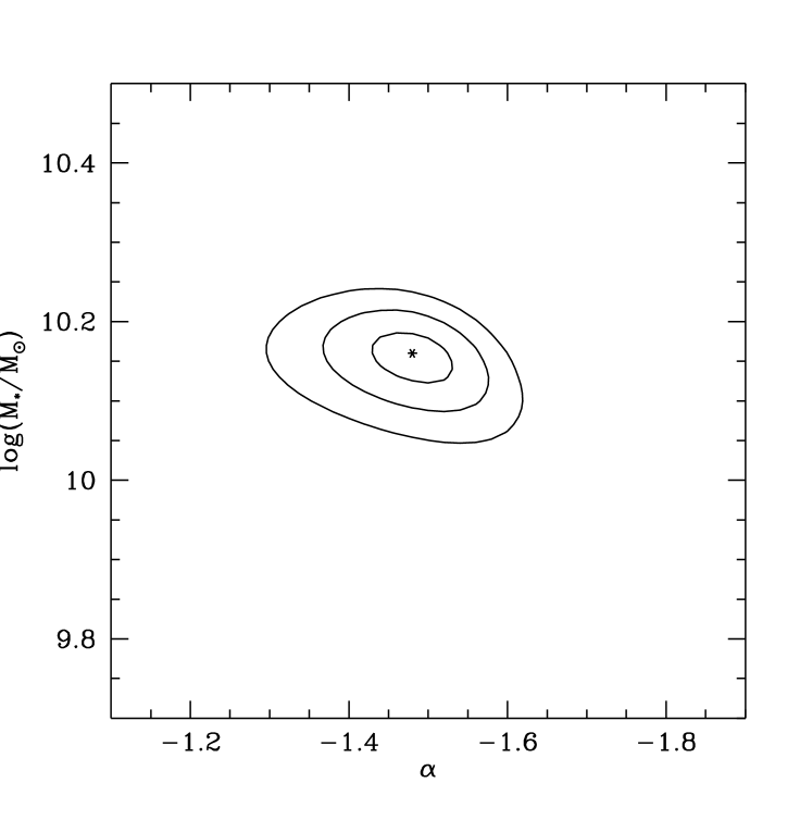
Figure 14: Contours of $\chi^{2}$ for pairs of our fit parameters are shown both before (top row) and after (bottom row) correction for galaxy density variations with distance. Contours are drawn at $\Delta\chi^{2}$ = 1, 4 and 9 corresponding to 1, 2 and 3$\sigma$ for one degree of freedom. The third parameter is kept fixed at the best-fitting value when plotting each pair.

The dotted line in Fig. 13 represents the approximate inverse search volume of our survey as function of mass, where we have assumed a relationship between H i mass and linewidth of the form: W${}_{20}\leavevmode\nobreak\ =\leavevmode\nobreak\ 0.16$ M${}_{\rm HI}^{1/3}$ km s^-1, for M_HI in solar units. The best-fitting Schechter functions of the form:

$$\Theta({\rm M})=\Theta_{*}{\rm ln}(10)({\rm M_{HI}}/{\rm M_{*}})^{\alpha+1}{\rm exp}(-{\rm M_{HI}/M_{*}}),$$

are over-laid on the data points. The straightforward (1/V_tot) points are best-fit with log(M_∗) = 10.15$\pm 0.1$, $\Theta_{*}$ = 9.5$\pm 3\times 10^{-4}$ and $\alpha$ = $-$1.5$\pm 0.1$, indicated by the dashed line in the figure. The best-fit values after correction for galaxy density as given by the upper panel of Fig. 11 are log(M_∗) = 9.85$\pm 0.07$, $\Theta_{*}$ = 55$\pm 15\times 10^{-4}$ and $\alpha$ = $-$1.28$\pm 0.1$, indicated by the solid line in the figure. Contours of $\chi^{2}$ for pairs of our fit parameters are shown in Fig. 14 both before and after correction for galaxy density variations with distance. The contours are drawn at $\Delta\chi^{2}$ = 1, 4 and 9 corresponding to 1, 2 and 3$\sigma$ for one degree of freedom. In each plot, the third parameter is kept fixed at the best-fitting value. From the $\chi^{2}$ contours it is clear that the solutions for log(M_∗) and $\alpha$ are well seperated, while combinations involving the galaxy density become somewhat degenerate.

For comparison the HIMF derived by Zwaan et al. (zwaa03 (2003)) from the HIPASS Bright Galaxy Catalog, based on 1000 H i selected galaxies in the $2\pi$ steradians below $\delta=0$, has log(M_∗) = 9.79$\pm 0.06$, $\Theta_{*}$ = 86$\pm 21\times 10^{-4}$ and $\alpha$ = $-$1.30$\pm 0.08$. Although completely at odds with our (1/V_tot) values, good agreement is apparent between these values and our own after application of the galaxy density correction. Similar considerations apply to HIMF derived by Rosenberg & Schneider (rose02 (2002)) from the Arecibo Dual-Beam Survey (ADBS) who find log(M_∗) = 9.88, $\Theta_{*}$ = 58$\times 10^{-4}$ and $\alpha$ = $-$1.53, although with somewhat poorer agreement in the faint end slope.

Although our choice of a minimum significance of 8$\sigma$ in integrated H i flux is expected to result in a high degree of completeness in our sample (cf. Rosenberg & Schneider rose02 (2002)), this can also be tested by evaluating the average value of V/V_max (Schmidt schm68 (1968)). For a complete sample of a uniform density volume we expect $<$V/V${}_{max}>$ = 0.5. In the absence of density corrections we actually find $<$V/V${}_{max}>$ = 0.35 for our sample, while after discrete density correction we find $<$V/V${}_{eff}^{\prime}>$ = 0.57, where D_max is based on the local 8$\sigma$ limit (which varies with distance as in Fig. 1) over a linewidth of 1.5$\times$W₂₀. If instead we define D_max by the local 8$\sigma$ limit over a linewidth of 1.2$\times$W₂₀ we obtain $<$V/V${}_{max}>$ = 0.31 and $<$V/V${}_{eff}^{\prime}>$ = 0.50. This may suggest that we have been somewhat too conservative in assessing significance based on the larger velocity intervals. However, a roll-off in completeness at the lowest significance levels can also result in an elevated expectation value of $<$V/V${}_{eff}>$ (Rosenberg & Schneider rose02 (2002)). Our value of $<$V/V${}_{eff}^{\prime}>$ = 0.57 is comparable to that found by Rosenberg & Schneider (rose02 (2002)) for the ADBS $<$V/V${}_{eff}>$ = 0.60.

4 Summary and Discussion

Our unbiased H i survey of 1800 deg² in the northern sky has allowed recognition of a number of significant points regarding the H i content, distribution and environment of nearby galaxies. From the analysis of some 500 candidate detections we have extracted a moderately complete sample of 155 galaxies (listed in Table 1 and illustrated in Fig. 3) with an integrated H i flux in excess of 8$\sigma$ at distances between 5 and 80 Mpc. Seven of the detections occur so near the boundary of our two segments of velocity coverage (near V_Hel = 2800 km s^-1), and two so near the edges of our spatial coverage, that their derived parameters are unreliable (although the detections themselves are secure). This leaves 146 detections with derived parameters of high quality. A plausible optical galaxy ID was found within a 30 arcmin search radius for all but one of the 8$\sigma$ detections, although one object was previously uncataloged and three others had no previous red-shift determination. Twenty-three objects (or their uncataloged companions) are detected in H i for the first time.

We have characterized the environment of each detected galaxy by performing a search within NED for all cataloged objects within a radius of 30 arcmin (corresponding to a possible contribution within our telescope beam). These (potential) companions have been tabulated in three categories in Table 1, namely; (a) confused for objects within 400 km s^-1 of the primary ID, (b) unconfused for objects offset by 400 to 1000 km s^-1 from the primary ID, and (c) possibly confused for objects of unknown red-shift. It will remain difficult to assess the actual liklihood of association for objects in this last category, until red-shift determinations become available. For the moment we will regard only those objects with entries in catgory (a) as “confused” and all others as “unconfused”.

We determine agreement of our absolute flux scale to the weighted average of all previous determinations of the H i flux (as tabulated by LEDA) to better than 1% for our unconfused detections, as shown in Fig. 7. Confused objects show a systematic excess H i flux in our large survey beam.

4.1 Centroid Offsets of Gas and Stars

Since our survey was not targeted at known galaxies, we have an independent determination of the position centroid for each detected object. The majority of apparent offsets between the gaseous and stellar distributions are consistent with the substantial uncertainties that follow from a large survey beam and only moderate signal-to-noise, as shown in Fig. 5. However, a number of significant centroid offsets (greater than 5$\sigma$) are detected in nominally unconfused galaxies which are indicated in Table 1 by entering the symbol “o”, “+” or “++” in the Note column. These have been divided somewhat arbitrarily into two categories, depending on whether the linear centroid offset is less than 10 kpc (category “o”) or greater than 10 kpc (categories “+” and “++”). The reasoning behind this division is that a 10 kpc limit may mark a plausible distinction between internal asymmetries of individual objects and the larger scales that are more likely to indicate external gaseous components.

Determining the cause of these significant centroid offsets requires higher resolution imaging. One extensive source of high resolution imaging is the WHISP survey (Kamphuis et al. kamp96 (1996), http://www.astro.rug.nl/w̃hisp) which has targeted some 200 UGC galaxies north of Dec = 20^∘ with synthesis observations using the WSRT array. WHISP observations are currently available for only a small fraction of the 155 galaxies in our 8$\sigma$ sample. The WHISP results for each galaxy are summarized in a web-accessible data overview consisting of a series of images of the integrated H i distribution and accompanying velocity field at three different angular resolutions, of about 15, 30 and 60 arcsec, together with a global H i profile, a major axis position-velocity plot and an optical reference image. The most relevant component of this overview for our purposes is the distribution of integrated H i at the lowest angular resolution of 60 arcsec, where the highest surface brightness sensitivity is reached. For the four of 11 instances of significant centroid offset noted in Table 1 that have already been imaged in the WHISP survey we comment briefly on what is seen in the 60 arcsec integrated H i image:

• NGC 7640 o : asymmetric with extensions.

• UGC 12732 o : possible companions.

• UGC 731 o : asymmetric.

• NGC 925 o : asymmetric with extensions.

All four cases that have been imaged with high resolution show large-scale asymmetries or possible uncataloged companions. Our tentative conclusion is that our measured centroid offsets are indeed indications of substantial asymmetries and the presence of possible uncataloged gas-rich companions in the immediate vicinity of the primary ID.

4.2 Uncataloged companions

The issue of uncataloged gas-rich companions is also addressed by the comparison of our survey flux densities with those measured previously for nominally unconfused galaxies in Figs. 8 and 9. Although the comparison with the heterogenous LEDA data has a large degree of scatter, the comparison with the Arecibo data may indicate an excess of H i at large radii.

The Arecibo data were taken from the Pisces-Perseus supercluster survey (Giovanelli & Haynes giov85 (1985), Giovanelli et al. giov86 (1986), Giovanelli & Haynes giov89 (1989), Wegner et al. wegn93 (1993) and Giovanelli & Haynes giov93 (1993)). We plot ratios of both the observed  and the corrected  H i flux density. In the latter case approximate corrections for telescope pointing errors and a model of the galaxy extent were applied to the Arecibo data. These data were only available for 20 of our unconfused detections, which vary in distance from about 7 to 70 Mpc. The Arecibo beam (3.3 arcmin FWHM at the time of those observations) has a linear dimension that varies from about 7 to 70 kpc over the distance range above, while our survey beam varies from about 100 kpc to 1 Mpc in diameter. Four of the unconfused galaxies have observed  flux ratios, $R$, of unity within our 1$\sigma$ errors, including the nearest object. All of the other galaxies have an excess detected H i flux in our larger survey beam which varies from about 10% to 300%. The comparison of corrected  flux ratios is more ambiguous, since at least five of the data-points now have apparent flux ratios which are significantly less than unity. As indicated in § 3 above, each of our survey detections was examined for evidence of source resolution effects and our absolute flux scale is well-defined, making such apparent deficits in our detected H i flux difficult to understand. Given the approximate nature of the corrections applied to the observed Arecibo fluxes it seems likely that they may (on occasion) result in a degree of over-compensation for missed flux.

The straightforward conclusion that can be drawn from the observed  flux ratio plots, it that in most cases, the H i distribution must be significantly more spatially extended than the Arecibo beam, even when this beam subtends 50–70 kpc.

High resolution imaging will be necessary to determine, on a case-by-case basis, where the excess detected flux actually resides. WHISP data (http://www.astro.rug.nl/w̃hisp) are currently available for 7 of the 20 unconfused galaxies that have Arecibo flux measurements. Inspection of the 60 arcsec integrated H i image in the WHISP database yields the following assessment:

• NGC 7286 : $R$=1.79, possible extensions.

• UGC 12693 : $R$=1.33, possible extensions.

• UGC 12713 : $R$=1.05, asymmetric.

• UGC 1856 : $R$=1.15, nothing unusual.

• NGC 972 : $R$=1.38, asymmetric, extensions, possible companions.

• NGC 1012 : $R$=1.21, 10% of H i flux in uncataloged companion.

• NGC 1056 : $R$=1.72, extensions.

The two cases showing the largest excess H i flux in the WSRT survey beam are notable for having possible extensions at low surface brightness in the distribution of integrated H i in the WHISP data. Only in one of these seven cases, has a distinct uncataloged companion been detected in the WHISP imaging. Deeper imaging of a larger field-of-view will be needed to search for additional uncataloged companions to account for the excess detected H i flux.

An intriguing possibility for the location of the excess detected H i flux is that it resides in a relatively diffuse distribution subtending a few 100 kpc in the vicinity of the primary target. This is exactly the type of hypothetical distribution, in the environment of M31, which motivated the negative velocity component of our wide-field H i survey. Such distributions were found (De Heij et al. dehe02 (2002)) to provide the best-fit to the spatial and kinematic distribution of the compact high–velocity cloud population in the vicinity of the Galaxy. The best-fitting models of this type consist of gas bound to low-mass dark-matter halos with a steep power-law ($\alpha=-1.7$) distribution in number as function of neutral gas mass and are concentrated around their major galaxy host in a Gaussian distribution with a spatial dispersion of 150–200 kpc. The total H i mass predicted in these Local Group models to survive (ram-pressure- and tidal-stripping) to the present day amounts to some 1.2$\times 10^{9}$M_⊙. Compared to the 8$\times 10^{9}$M_⊙ of H i in M31 and the Galaxy, this corresponds to an excess H i mass of about 15% distributed on scales of a few hundred kpc. Only a handful of the rare, massive components might be identifiable as discrete objects, while the rest of the distribution would merely contribute to a diffuse enhancement of H i mass, centered on the systemic velocity of the host.

This possibility can and should be tested with a dedicated experiment.

4.3 Spatial Variance of the HIMF

In §3 we derive an HIMF from our 8$\sigma$ sample of background galaxies. Despite the fact that our survey region covered some 1800 deg² and therefore sampled a variety of environments along the line-of-sight, it is impossible to overcome the fact that in a flux-density limited sample, all low mass detections must of necessity be very nearby. In consequence, the power-law slope and normalization of the HIMF are strongly dependent on whether or not there are significant variations of the average galaxy density with distance. We have quantified such a variation by utilizing cataloged optical galaxies in our survey volume as shown in Figs. 10 and 11. The absolute density of optical galaxies as function of distance was determined by fitting for the normalization of the “standard” luminosity function determined by Norberg et al. (norb02 (2002)) in a sequence of heavily over-lapping sub-samples. Density variations with distance of more than an order of magnitude are derived within our survey volume. Accounting for this variation leads to very substantial changes in the best-fitting HIMF parameters, as seen in Fig. 13. Before correction we obtain log(M_∗) = 10.15$\pm 0.1$, $\Theta_{*}$ = 9.5$\pm 3\times 10^{-4}$ and $\alpha$ = $-$1.5$\pm 0.1$, and after correction log(M_∗) = 9.85$\pm 0.07$, $\Theta_{*}$ = 55$\pm 15\times 10^{-4}$ and $\alpha$ = $-$1.28$\pm 0.1$, where the error estimates come from the 2$\sigma$ contours of $\Delta\chi^{2}$ in the fit parameters shown in Fig. 14.

Only after applying the density correction is statistical agreement realized with the HIPASS BGC values (Zwaan et al. zwaa03 (2003)) log(M_∗) = 9.79$\pm 0.06$, $\Theta_{*}$ = 86$\pm 21\times 10^{-4}$ and $\alpha$ = $-$1.30$\pm 0.08$ and to a lesser extent with the Arecibo Dual-Beam Survey (ADBS) values (Rosenberg & Schneider rose02 (2002)) log(M_∗) = 9.88, $\Theta_{*}$ = 58$\times 10^{-4}$ and $\alpha$ = $-$1.53.

Schneider et al. (schn98 (1998)) and Rosenberg & Schneider (rose02 (2002)) also consider the variation of number density of optical galaxies in the ADBS survey region. However they determine only a relative, rather than an absolute density and do so on the basis of galaxy number counts rather than explicit fitting to the complete portion of the luminosity function. They conclude that density corrections have only a minor impact on the form and normalization of the HIMF in their sample, although their normalization does increase from 48 to 58$\times 10^{-4}$ (Mpc^-3dex^-1), when relative density corrections are applied. These authors also make use of the “integral” formulation of density correction discussed in §3 rather than the “discrete” formulation which we find leads to substantially reduced fit residuals.

The absolute normalization of the HIPASS BGC HIMF is not a trivial procedure (Zwaan et al. zwaa03 (2003)). Since a maximum likelihood method has been employed, the shape if the HIMF should be well-determined, but only in terms of a relative density. The normalization is determined after the fact by carrying out integrations of the derived selection function. Since a reasonable range of detected masses in the HIPASS sample is only achieved inside of about 25 Mpc, the normalization is, of necessity, also tied to this distance range. To assess the impact of a possible variation of galaxy density with distance within the HIPASS sample, we have also fit for the optical galaxy normalization using all LEDA galaxies at $\delta<0$, just as in §3, for our own survey volume. Given the larger optical galaxy sample size, we defined 25 overlapping sub-samples with sample populations varying linearly from a minumum of 100 galaxies at the nearest distances to 1500 galaxies at the maximum distance. This distribution is plotted as the dotted line in Fig.11. The southern hemisphere has a galaxy density which is equal to the Norberg et al. (norb02 (2002)) value between about 8 and 25  Mpc. At larger distances there appears to be a smooth decline to about 30% of this density by 80 Mpc. At distances smaller than about 8 Mpc there also appears to be a decline in galaxy density to about 50% of nominal. It seems that over the critical distance range of 10–25 Mpc, the galaxy density within the HIPASS survey volume is essentially the nominal one, suggesting that the HIPASS BGC value of $\Theta_{*}$ = 86$\pm 21\times 10^{-4}$ Mpc^-3dex^-1 should be quite reliable. The apparent down-turn in galaxy density below about 8 Mpc may have some consequence for the apparent shape of the HIPASS BGC HIMF below log(M) = 7.5, since such systems could only be detected out to 8 Mpc in the HIPASS data.

For comparison we have also determined and plotted the optical galaxy density in the same way for the entire northern hemisphere in Fig.11. The northern hemisphere distribution is quite different than the southern, with a moderate over-density (about 50 %) inside of 15 Mpc, followed by a relative dearth of galaxies between 20 and 60 Mpc. It seems quite conceivable that the apparent discrepancies between the HIPASS BGC and the ADBS HIMF parameters may be a consequence of such large-scale differences in the galaxy distribution.

- (1) Barnes, D. G., Staveley–Smith, L., de Blok, W. J. G., et al., 2001, MNRAS, 322, 486
- (2) Braun, R., Burton, W. B., 1999, A&A, 341, 437
- (3) Chamaraux, P., Balkowski, C., Fontanelli, P., 1987, A&ASS, 69, 263
- (4) de Heij, V., Braun, R., Burton, W. B., 2002, A&A, 392, 417
- (5) Ferguson, A. M. N., Gallagher, J. S., Wyse, R. F. G., 2000, AJ, 120, 821
- (6) Gooch, R., 1995, in ASP Conf Ser. 77, Astronomical Data Analysis Software and Systems IV, ed. R.A. Shaw, H.E. Payne, & J.E. Haynes (San Franciso: ASP), 144
- (7) Hartmann, D., Burton, W. B., 1997, Atlas of Galactic Neutral Hydrogen, Cambridge University Press
- (8) Giovanelli, R., Haynes, M. P., 1985, AJ, 90, 2445
- (9) Giovanelli, R., Haynes, M. P., Myers, S. T., Roth, J., 1986, AJ, 92, 250
- (10) Giovanelli, R., Haynes, M. P., 1989, AJ, 97, 633
- (11) Giovanelli, R., Haynes, M. P., 1993, AJ, 105, 1271
- (12) Haynes, M. P., Herter, T., Barton, A. S., Benensohn, J. S., 1990, AJ, 99, 1740
- (13) Kamphuis, J. J., Sijbring, L. G., van Albada, T. S., 1996, A&AS, 116, 15
- (14) Kilborn, V. A., Webster, R. L., Staveley–Smith L., et al., 2002, AJ, 124, 690
- (15) Lang, R. H., Boyce, P. J., Kilborn, V. A., et al., 2003, MNRAS, in press, (astro-ph/0302317)
- (16) Norberg, P., Cole, S., Baugh, C. M., et al., 2002, MNRAS, 336, 907
- (17) Putman, M. E., de Heij, V., Stavely–Smith, L., et al., 2002, AJ, 123, 873
- (18) Rosenberg, J. L., Schneider, S. E., 2002, ApJ, 567, 247
- (19) Saunders, W., Rowan-Robinson, M., Lawrence, A., et al., 1990, MNRAS, 242, 318
- (20) Schlegel, D. J., Finkbeiner, D. P., Davis, M., 1998, ApJ, 500, 525
- (21) Schneider, S. E., Thuan, T. X., Mangum, J. G., Miller, J., 1992, ApJS, 81, 5
- (22) Schneider, S. E., Spitzak, J. G., Rosenberg, J. L., 1998, ApJ, 507, L9
- (23) Schmidt, M., 1968, ApJ, 151, 393
- (24) Theureau, G., Bottinelli, L., Coudreau-Durand, N. et al. 1998, A&AS, 130, 1
- (25) Vennik, J., Richter, G. M., 1994, Astron.Nachr., 315, 245
- (26) Vorontsov-Velyamonov, B. A., 1977, A&AS, 28, 1
- (27) York, D. G., Adelman, J., Anderson, J. E., et al., 2000, AJ, 120, 1579
- (28) Wegner, G., Haynes, M. P., Giovanelli, R., 1993, AJ, 105, 1251
- (29) Zwaan, M. A., Staveley–Smith L., Koribalski, B. S., et al., 2003, AJ, in press (astro-ph/0302440)
- (30) Zwaan, M. A., Briggs, F. H., Sprayberry, S., Sorar, E., 1997, ApJ 490, 173