3-point temperature anisotropies in WMAP:
Limits on CMB non-Gaussianities and non-linearities

Abstract

We present a study of the 3-pt angular correlation function $w_{3}=<\delta_{1}\delta_{2}\delta_{3}>$ of (adimensional) temperature anisotropies measured by the Wilkinson Microwave Anisotropy Probe (WMAP). Results can be normalized to the 2-point function $w_{2}=<\delta_{1}\delta_{2}>$ in terms of the hierarchical: $q_{3}\sim w_{3}/w_{2}^{2}$ or dimensionless: $d_{3}\sim w_{2}/w_{2}^{3/2}$ amplitudes. Strongly non-Gaussian models are generically expected to show $d_{3}>1$ or $q_{3}>10^{3}d_{3}$. Unfortunately, this is comparable to the cosmic variance on large angular scales. For Gaussian primordial models, $q_{3}$ gives a direct measure of the non-linear corrections to temperature anisotropies in the sky: $\delta=\delta_{L}+f_{NLT}(\delta_{L}^{2}-<\delta_{L}^{2}>)$ with $f_{NLT}=q_{3}/2$ for the leading order term in $w_{2}^{2}$. We find good agreement with the Gaussian hypothesis $d_{3}\sim 0$ within the cosmic variance of $\Lambda$CDM simulations (with or without a low quadrupole). The strongest constraints on $q_{3}$ come from scales smaller than 1 degree. We find $q_{3}=19\pm 141$ for (pseudo) collapsed configurations and an average of $q_{3}=336\pm 218$ for non-collapsed triangles. The corresponding non-linear coupling parameter, $f_{NL}$, for curvature perturbations $\Phi$, in the Sachs-Wolfe (SW) regime is: $f_{NL}^{SW}=q_{3}/6$, while on degree scales, the extra power in acoustic oscillations produces $f_{NL}\sim q_{3}/30$ in the $\Lambda$CDM model. Errors are dominated by cosmic variance, but for the first time they begin to be small enough to constrain the leading order non-linear effects with coupling of order unity.

I Introduction

We study the cosmic microwave background (CMB) anisotropies measured by WMAP (Ben03, ) from the point of view of the 3-point angular correlation $w_{3}$. Current models for structure formation predict that the initial seeds, that later give rise to the observed structure in the universe , were Gaussian. If so, one would expect the angular 3-point CMB temperature correlations to be almost zero. Even for a Gaussian field, any non-linear processing of the primordial perturbations would lead to small non-Gaussianities. For an excellent review see (Kom03, ) and references therein.

Angular correlations have some advantages over spherical harmonic analyses. The main disadvantage is that different angular bins are highly correlated, which means that we need to use the full covariance matrix to assess the significance of any departures between measurements and models. The advantage of using the N-point function is that correlations can be easily sampled from any region of the sky, even when a foreground mask is required, provided the region is large enough. In comparison, harmonic decomposition breaks the angular symmetry in the sky into orthogonal bases which have an arbitrary phase orientation. This is not a problem in the case of full sky coverage, but the results will be coordinate-dependent if a mask is used. Moreover, higher order correlations, such as the bispectrum, have to focus on some small portion of the mutidimensional space of triangle configurations (see (Kom03, )). The formal equivalence between the bispectrum and the 3-point function is hardly realized in practice and as such it is of interest to study both separately.

Our analysis procedure is similar to that presented in (Gaz03, ), to which the reader can refer for further details. We use the same simulations where we’ve generated maps using the standard $\Lambda$CDM model and a low-Q $\Lambda$CDM model, a fiducial variation of the $\Lambda$CDM model with low values of the quadrupole and octopole. We concentrate our analysis on the V-band WMAP maps (FWHM = 21’ at 61 GHz) generated using HEALPix (Gor99, ) with pixel resolution n=512 (7’ pixels) and to which we apply the conservative WMAP kp0 foreground mask (Ben03, ), The resulting maps have approximately 2.4 million pixels.

II Correlation functions from WMAP

The 2-point angular correlation function is defined as the expectation value or mean cross-correlation of temperature fluctuations:

$$\mbox{$$}\delta({\bf q})\equiv{\Delta T({\bf q})\over{T_{0}}}$$ (1)

at two positions ${\bf q}_{1}$ and ${\bf q}_{2}$ in the sky:

$$\mbox{$$}w_{2}(\theta)\equiv\langle\delta({\bf{\bf q}_{1}})\delta({\bf{\bf q}_{2}})\rangle,$$ (2)

where $\theta=|\bf{{\bf q}_{2}}-\bf{{\bf q}_{1}}|$, assuming that the distribution is statistically isotropic. We normalize fluctuations to be dimensionless, $T_{0}=2.73$K, or dimensional with $T_{0}=1$. To estimate $w_{2}(\theta)$ from the pixel maps we use:

$$\mbox{$$}w_{2}(\theta)={\sum_{i,j}\delta_{i}\delta_{j}~{}w_{i}~{}w_{j}\over{\sum_{i,j}w_{i}~{}w_{j}}},$$ (3)

where $\delta_{i}$ and $\delta_{j}$ are the observed temperature fluctuations on the sky and the sum extends to all pairs $i,j$ separated by $\theta\pm\Delta\theta$. The mean temperature fluctuation is subtracted so that $\langle\delta_{i}\rangle=0$. The weights $w_{i}$ can be used to minimize the variance when the pixel noise is not uniform, however this introduces larger cosmic variance. Here we follow the WMAP team and use uniform weights (i.e. $w_{i}=1$). At the largest scales we use bins $\Delta\theta$ whose size is proportional to the square root of the angle $\theta$ and use linear bins of $\Delta\theta\simeq 0.26$ degrees at the smallest scales.

II.1 3-point function

In a similar fashion, the 3-point angular correlation function is defined as the cross-correlation of temperature fluctuations at 3 positions ${\bf q}_{1}$, ${\bf q}_{2}$ and ${\bf q}_{3}$ on the sky:

$$\mbox{$$}w_{3}(\theta_{12},\theta_{13},\theta_{23})\equiv\langle\delta({\bf{\bf q}_{1}})\delta({\bf{\bf q}_{2}})\delta({\bf{\bf q}_{3}})\rangle,$$ (4)

where $\theta_{ij}=|\bf{{\bf q}_{i}}-\bf{{\bf q}_{j}}|$. Consider a triplet of pixels with labels 1,2,3 on the sky. Let $\theta_{12}$ and $\theta_{13}$ be the angular separations between the corresponding pairs of pixels and $\alpha$ the interior angle between these two sides of the triangle. Assuming that the distribution is statistically isotropic, $w_{3}$ only depends on the sides of the triangles that define the 3 positions on the sky. One can characterize the configuration-dependence of the three-point function by studying the behavior of $w_{3}(\alpha)$ for fixed $\theta_{12}$ and $\theta_{13}$.

To estimate $w_{3}(\theta_{12},\theta_{13},\theta_{23})$ from the pixel maps we use:

$$\mbox{$$}w_{3}(\theta_{12},\theta_{13},\theta_{23})={\sum_{i,j,k}\delta_{i}\delta_{j}\delta_{k}~{}w_{i}~{}w_{j}~{}w_{k}\over{\sum_{i,j,k}w_{i}~{}w_{j}~{}w_{k}}},$$ (5)

where $\delta_{i}$, $\delta_{j}$ and $\delta_{k}$ are the temperature differences in the map and the sum extends to all triplets separated by $\theta_{12}\pm\Delta\theta$, $\theta_{13}\pm\Delta\theta$ and $\theta_{23}\pm\Delta\theta$. We use same bins and weights as in the 2-point function above.

The 3-point function can either be normalized to a dimensionless amplitude:

$$\mbox{$$}d_{3}\equiv{w_{3}\over{(w_{12}w_{23}w_{13})^{3/2}}}$$ (6)

where $w_{ij}=w_{2}(\theta_{ij})$, or a hierarchical amplitude:

$$\mbox{$$}q_{3}\equiv{w_{3}\over{w_{12}w_{23}+w_{12}w_{13}+w_{23}w_{13}}}.$$ (7)

II.2 Errors

The covariance matrix between different angular bins can be calculated from the simulations:

$$\mbox{$$}C_{ij} \equiv \langle\Delta w_{2}(\theta_{i})~{}\Delta w_{2}(\theta_{j})\rangle$$ (8)

$$= {1\over{N}}\sum_{L=1}^{N}\Delta w_{2}^{L}(\theta_{i})\Delta w_{2}^{L}(\theta_{j}),$$

where $\Delta w_{2}^{L}(\theta_{i})\equiv w_{2}^{L}(\theta_{i})-\widehat{w_{2}}(\theta_{i})$. Here $w_{2}^{L}(\theta_{i})$ is the 2-point or 3-point function measured in the $L$-th realization ($L=1\dots N$) and $\widehat{w_{2}}(\theta_{i})$ is the mean value for the $N$ realizations. The case $i=j$ gives the error variance: $\sigma_{i}^{2}\equiv C_{ii}$.

An estimate of the errors for correlations measured on the real sky can be obtained using a variation of the jackknife error scheme. This has the potential advantage of producing an error estimate which is model independent. The accuracy of the jack-knife covariance have been tested for both WMAP (Gaz03, ) and the APM and SDSS survey (Scranton et al., 2002), (Gaztañaga, 2002), (Gaztañaga, 2002). In the estimation, the sample is first divided into $M$ separate regions on the sky, each of equal area. The analysis is then performed $M$ times, on each occasion removing a different region. These are called the (jackknife) subsamples, which we label $k=1\dots M$. The estimated statistical covariance for $w_{2}$ at scales $\theta_{i}$ and $\theta_{j}$ is then given by:

$$\mbox{$$}C_{ij} = {M-1\over{M}}\sum_{k=1}^{M}\Delta w_{2}^{k}(\theta_{i})\Delta w_{2}^{k}(\theta_{j})$$ (10)

$$\Delta w_{2}^{k}(\theta_{i})\equiv w_{2}^{k}(\theta_{i})-\widetilde{w_{2}}(\theta_{i})$$

where $w_{2}^{k}(\theta_{i})$ is the measure 2 or 3-point function in the $k$-th subsample ($k=1\dots M$) and $\widetilde{w_{2}}(\theta_{i})$ is the mean value for the $M$ subsamples. The case $i=j$ gives the error variance. Note how, if we increase the number of regions $M$, the jackknife subsamples are larger and each term in the sum is smaller. We typically take $M=8$ corresponding to a division of the sphere into 8 octants. Note that the 3-point correlation function is in general a function of 3 variables. We will fix two of these variables and show variations of $w_{3}$ or $q_{3}$ as a function of a single variable, for which we estimate the covariance with the above prescription.

II.3 The algorithm

Estimation of correlations in configuration space is quite time consuming. A brute force algorithm to estimate all pair separations in a map with $N$ pixels takes $\simeq N^{2}$ operations. To do all triplets in Eq.[5] we need $\simeq N^{3}$ operations. In the healpix $n=512$ WMAP maps (7 arcmin pixel’s) we have $N\simeq 2.4\times 10^{6}$ (with the Kp0 mask galactic cut) so a brute force analysis requires $\simeq 10^{20}$ operations, well beyond current computing power. We overcome this difficulty in two steps. For large scales, $\theta>1$ degree, we reduce the resolution of the maps to $n=64$ (1 degree resolution) by averaging fluctuations over nearby pixels. The resulting correlation function contains the same information at scales larger than the new resolution scale. Now the number of pixels is reduced to $N=3\times 10^{4}$ and the number of operations to $\simeq 10^{13}$, which lies within current computer power (Teraflops). For scales smaller than a few degrees we can reduce the number of operations by precalculating the distance between neighboring pixels. The number of operations is then reduced to $N\times M^{2}$, where $M<<N$ is the number of neighbors. In our case we have $M\simeq 10^{3}$ for pixels around $\theta<4$ degrees, and thus $N\times M^{2}\simeq 10^{13}$ as in the case for the larger angles. In our implementation we have an overlap between the large and small scale estimations at around $2-4$ degrees. The agreement between both estimates here is quite good for both $w_{2}$ and $w_{3}$. In the case of the 2-point function we have compared both estimates in the whole range $2-180$ degrees and find excellent agreement.

II.4 Results

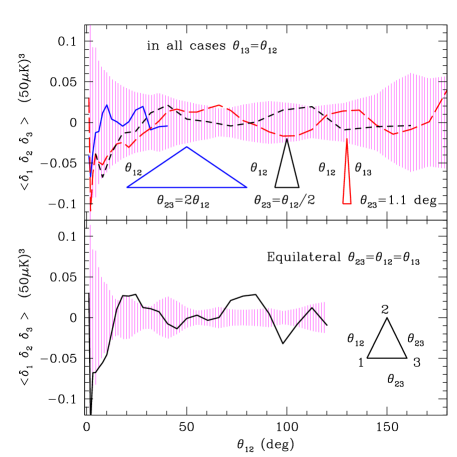
Figure 1: 3-point function $w_{3}=<\delta_{1}\delta_{2}\delta_{3}>$ at large angular scales. Bottom spanel shows $w_{3}$ for equilateral triangles as a function of side $\theta_{12}$. The top panel shows results for isosceles triangles $\theta_{13}=\theta_{12}$ with $\theta_{23}=1.1deg$ (long dashed line), $\theta_{23}=\theta_{12}/2$ (short dashed line) and $\theta_{23}=2\theta_{12}$ (continuous line), in all cases as a function of side $\theta_{12}$. Shaded regions are for the 68% confidence levels estimated using jackknife errors.

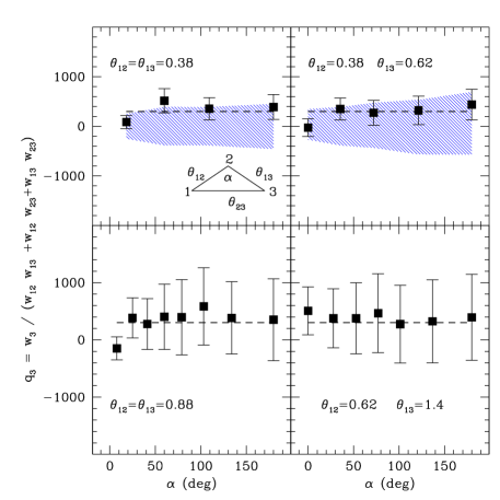
Figure 2: Reduced 3-point function $q_{3}$ at small angular scales. Different panels show configurations with triangles of fixed sides $\theta_{12}$ and $\theta_{13}$ (as labeled in each panel) and variable $\theta_{23}$ which is given by the interior angle $\alpha$ between $\theta_{12}$ and $\theta_{13}$ ($\alpha=0$ corresponds to $\theta_{23}=0$ and $\alpha=180$ corresponds to $\theta_{23}=2\theta_{12}$). Shaded regions are for the 68% confidence levels estimated using low-Q $\Lambda$CDM simulations. Errorbars are from jackknife variance.

Results are presented in Figures 1 and 2. At large scales Fig.1 shows the results of $w_{3}$ in units of $(50\mu K)^{3}$ (eg $T_{0}=50\mu K$ in Eq.[1]). Note that $w_{2}^{1/2}\simeq 50\mu K$ at small scales, so that $w_{3}\simeq d_{3}\equiv w_{3}/w_{2}^{3/2}$ in these units (see Eq.[6]). Errorbars in both cases are from jackknife subsamples and agree well with errors estimated from the simulations (see Gaztañaga etal 2003 for more details). The results for the equilateral and collapsed triangle configurations can be compared to the COBE analysis presented in Fig.1 of (Kog96, ). The pseudo-collapsed case in (Kog96, ) would correspond here to $\theta_{23}=1.1deg$ here. We can see how the COBE and WMAP results are in good agreement where the two curves even see the very same bumps and valleys. This is not totally surprising given the very good match between COBE and WMAP temperatures maps, pixel by pixel, when smoothed on large scales. The top panel in Figure 1 also shows two new triangle configurations: one that is elongated, $\theta_{23}=\theta_{12}/2$ (short dashed line), and a wide triangle, $\theta_{23}=2\theta_{12}$ (continuous line). The results for intermediate angular configurations are similar. In all cases the agreement with the Gaussian prediction $w_{3}=0$ is excellent, given the strong covariance.

At small scales we show the 3-point function in terms of the reduced amplitude $q_{3}$ in Eq.[7] where the best constraints are found on the smallest scales. As can be seen in the figure, as we approach triangles with side $\theta\simeq 1$degree, the cosmic errors become large $\Delta q_{3}\simeq 1000$. We have fit the data to a constant value of $q_{3}$, independent of scale using a $\chi^{2}$-test:

$$\mbox{$$}\chi^{2}=\sum_{i,j=1}^{N}\Delta_{i}~{}C_{ij}^{-1}~{}\Delta_{j},$$ (11)

where $\Delta_{i}\equiv q_{3}^{O}(\alpha_{i})-q_{3}^{fit}$ is the difference between the ”observation” $O$ and the $fitted$ value. In order to eliminate the degeneracies in the covariance matrix, we perform a Singular Value Decomposition (SVD) of the covariance matrix (see Gaztañaga et al. 2003 for more details). A joint fit with the jackknife covariance matrix for collapsed configurations with $\theta<1$ degree, yields:

$$\mbox{$$}q_{3}^{collapsed}=19\pm 141.$$ (12)

The best signal-to-noise is found for the non-collapsed triangle configurations with $\theta\simeq 0.5$ degree we find:

$$\mbox{$$}q_{3}=336\pm 218~{}~{}~{}~{}~{}~{}~{};~{}~{}~{}~{}\theta=0.5~{}deg$$ (13)

providing a marginal detection at about 90% confidence (shown as dashed line in Fig.2). This fit corresponds to the jackknife covariance matrix. A similar result is found for the covariance matrix in the low-q $\Lambda$CDM simulations. The errors increase by almost a factor of two when using the covariance of the standard $\Lambda$CDM simulations. This increase is due to the larger cosmic variance introduced by the quadrupole and octopole which are larger than in the WMAP data (see (Spe03, ), citepGaz03 for a discussion).

III Discussion

The above results for the 3-pt function confirms previous analyses ((Kom03, ) and references therein) that find WMAP to be in good agreement with the Gaussian hypothesis. Strong non-Gaussian statistics with $d_{3}$ in Eq.[6] of order unity or larger are ruled out. On larger (COBE) angular scales the results are dominated by cosmic variance so that $\Delta d_{3}\simeq 1$ (Sre93, ) and $\Delta q_{3}\simeq 1000$. On subdegree scales errors are smaller and we find evidence for a marginal detection (90% level) of non-Gaussianity in Eq.[13]. This result can be taken as a detection or, at a higher significance level, a bound on possible non-linear effects. Expanding the observed temperature fluctuation $\delta$ as a perturbation over some primordial Gaussian linear contribution $\delta_{L}$:

$$\mbox{$$}\delta=\delta_{L}+f_{NLT}~{}(\delta_{L}^{2}-<\delta_{L}^{2}>),$$ (14)

we then have that to leading order in $w_{2}$:

$$\mbox{$$}w_{3}=2~{}f_{NLT}~{}(w_{12}w_{23}+w_{12}w_{13}+w_{23}w_{13})+{\cal O}[w_{2}^{4}]$$ (15)

so that $q_{3}\simeq 2~{}f_{NLT}$. The corresponding non-linear coupling parameter, $f_{NL}$, for curvature perturbations $\Phi$ is:

$$\mbox{$$}\Phi=\Phi_{L}+f_{NL}~{}(\Phi_{L}^{2}-<\Phi_{L}^{2}>).$$ (16)

In the Sachs-Wolfe (SW) regime ($\delta\sim\Phi/3$) we have: $f_{NL}^{SW}\simeq q_{3}/6$, while on degree scales, the extra power in acoustic oscillations produce $f_{NL}\simeq q_{3}/30$ in the case of $\Lambda$CDM KS01 . This corresponds to $f_{NL}\simeq 11.2\pm 7.3$ for Eq.[13] and $f_{NL}\simeq 0.6\pm 4.7$ for the collapsed case Eq.[12]. For a comparison with recent predictions see (Kom03, ; BU02, ; Acq02, ; Mal02, ; Zal03, ) and references therein.

Our bounds on $f_{NL}$ seem marginally better than the ones presented in (Kom03, ) from the WMAP bispectrum, but a direct comparison is not straight forward. First of all, our modelling provides a measurement of non-linearities in the final $\Delta T$ while (Kom03, ) provide a modelling for non-linear primordial curvature perturbations $\Phi$, before radiation transfer. Thus while limits on $q_{3}$ are model independent, direct limits on $f_{NL}$ depend on the assumed model for radiation transfer. Secondly, the bispectrum configurations used by (Kom03, ) are a subset of all possible triangle configurations so that both approaches are neither equivalent nor optimized in the same way. In both cases, errors are dominated by cosmic variance, and they begin to be small enough to constrain the leading order non-linear effects with coupling $f_{NL}$ which are of order unity.

- (1) Bennett C.L. et al. , 2003, preprint (astro-ph/0302207).
- (2) Komatsu, E. et al. 2003, preprint (astro-ph/0302223).
- (3) Gaztañaga, E, Wagg, J., Multamäki, T., Montaña, A., Hughes, D.H., 2003, submitted to MNRAS (astro-ph/0304178).
- (4) Górski, K. M., Hivon, E., & Wandelt, B. D., 1999, in Proceedings of the MPA/ESO Cosmology Conference ”Evolution of Large-Scale Structure”, eds. A.J. Banday, R.S. Sheth and L. Da Costa, PrintPartners Ipskamp, NL, pp. 37-42 (also astro-ph/9812350).
- Scranton et al. (2002) Scranton, R. et al. 2002, ApJ, 579, 48
- Gaztañaga (2002) Gaztañaga, E. 2002, MNRAS, 333, L21
- Gaztañaga (2002) Gaztañaga, E. 2002, ApJ, 580, 144
- (8) Kogut A., Banday A.J., Bennett C.L., Gorski K.M., Hinshaw G., Smoot G.F., Wright E.L., 1996, ApJ, 464, L29.
- (9) Spergel D.N. et al. , 2003, preprint (astro-ph/0302209).
- (10) Srednicki, M., 1993, ApJ, 416, L1
- (11) Komatsu, E., Spergel, D., 2001, PhRvD 63, 063002
- (12) Acquaviva, V., Bartolo, N., Matarrese, S., Riotto, A. 2003, preprint (astro-ph/0209156).
- (13) Bernardeau, F., Uzan, J-P., 2002, preprint (astro-ph/0209330).
- (14) Maldacena, J., preprint (astro-ph/0210603).
- (15) Zaldarriaga, M., preprint (astro-ph/0306006).