Red and Reddened Quasars in the Sloan Digital Sky Survey

Abstract

We investigate the overall continuum and emission line properties of quasars as a function of their optical/UV spectral energy distributions. Our sample consists of 4576 quasars from the Sloan Digital Sky Survey (SDSS) that were chosen using homogeneous selection criteria. Expanding on our previous work which demonstrated that the optical/UV color distribution of quasars is roughly Gaussian, but with a red tail, here we distinguish between 1) quasars that have intrinsically blue (optically flat) power-law continua, 2) quasars that have intrinsically red (optically steep) power-law continua, and 3) quasars whose colors are inconsistent with a single power-law continuum. We find that 273 (6.0%) of the quasars in our sample fall into the latter category and appear to be redder because of SMC-like dust extinction and reddening rather than because of synchrotron emission. Even though the SDSS Quasar Survey is optically selected and flux-limited, we demonstrate that it is sensitive to dust reddened quasars with $E(B-V)\lesssim 0.5$ assuming a classical Small Magellanic Cloud (SMC) extinction curve. The color distribution of our SDSS quasar sample suggests that the population of moderately dust reddened, but otherwise normal (i.e., Type 1) quasars is smaller than the population of unobscured quasars: we estimate that a further 10% of the quasar population with $M_{i}<-25.61$ is missing from the SDSS sample because of extinction, bringing the total fraction of dust reddened quasars to 15% of broad-line quasars.

We also investigate the emission and absorption line properties of these quasars as a function of color and comment on how some of these results relate to Boroson & Green type eigenvectors. Quasars with intrinsically red (optically steep) power-law continua tend to have narrower Balmer lines and weaker C IV, C III], He II and $3000\,{\rm\AA}$ bump emission as compared with bluer (optically flatter) quasars. The change in strength of the $3000\,{\rm\AA}$ bump appears to be dominated by the Balmer continuum and not by Fe II emission. The dust reddened quasars have even narrower Balmer lines and weaker $3000\,{\rm\AA}$ bumps, in addition to having considerably larger equivalent widths of [O II] and [O III] emission. The fraction of broad absorption line quasars (BALQSOs) increases from $\sim 3.4\%$ for the bluest quasars to perhaps as large as $20\%$ for the dust reddened quasars, but the intrinsic color distribution will be much bluer if all BALQSOs are affected by dust reddening.

1 Introduction

The existence of a significant population of red quasars has been the subject of debate for a number of years. The color distribution of quasars (Webster et al. 1995; Francis, Whiting, & Webster 2000; Brotherton et al. 2001; Richards et al. 2001) and the discovery of a few examples of highly reddened radio-selected quasars (Gregg et al. 2002; White et al. 2003) strongly suggest that a sizeable population of such objects does indeed exist. Nevertheless, it is still unclear how often different mechanisms (e.g., dust extinction, a synchrotron emission turnover, or simply intrinsic continuum differences) are at work, whether this class of objects is a significant fraction of the total quasar population, and whether moderately dust reddened Type 1 quasars are significant contributors to the X-ray background (Mushotzky et al. 2000; Brandt et al. 2000) — independent of the contribution of Type 2 quasars with completely obscured broad emission line regions (BELRs).

Part of the reason that these issues are not better understood may be the heterogeneous definitions that have been used to classify quasars as “red”. This paper suggests that traditional samples of red quasars that impose cuts on observed colors or spectral index (e.g., Webster et al. 1995; Francis et al. 2001; Wilkes et al. 2002; Gregg et al. 2002) are too heterogeneous with redshift to yield physically homogeneous samples of red quasars. Spectral indices are sensitive to the choice of continuum windows, and simple color cuts necessarily ignore the significant contribution that emission and absorption lines make to the colors of quasars as a function of redshift. That is not to say that such red quasar criteria are not reasonable, but rather that care must be taken in the interpretation of such samples after the fact. Herein we address these issues with a sample of quasars from the Sloan Digital Sky Survey (SDSS; York et al. 2000). Using this sample, we present a more redshift-independent selection criterion for red quasars that allows for better classification of the types (and causes) of red quasars, which, in turn, will lead to a better census of the quasar population in the future.

We demonstrate that the distribution of optical colors of normal quasars is resolved by the SDSS and we isolate quasars as a function of optical color. The majority of our quasars are consistent with a roughly Gaussian distribution in color that can be characterized by a Gauassian distribution in spectral index. For these quasars, which have colors that are roughly consistent with a single power-law continuum, the fact that our photometric errors are smaller than the width of the distribution allows us to differentiate between those quasars that have bluer than average colors (hereafter referred to as “optically flat” quasars) and quasars that have slightly redder than average color — but still blue in an absolute sense — hereafter referred to as “optically steep” quasars. In addition, there is a red tail to the distribution beyond that which can be explained by a Gaussian distribution in spectral index. These quasars that have continua with curvature that cannot be explained by a single power-law slope; they appear reddened as a result of a decrement of blue flux such as might result from dust extinction and are referred to hereafter as “dust reddened” quasars. Quasars can also appear redder than average as a result of an excess of red flux such as might result from the presence of a synchrotron source with a high-frequency turnover in the rest-frame UV or optical, such quasars are referred to hereafter as “red synchrotron” quasars; Serjeant & Rawlings 1997; Francis et al. 2000). See § 3.2 and § 4.1 for figures that help with visual clarification of our flat/steep/dusty nomenclature.

Our analysis of reddened quasars discusses whether the heavily reddened quasars in the literature are just the tail of a population dominated by less reddened quasars, or if there is an equal distribution of extreme, moderate, and mild reddening, or if the distribution is bimodal with reddening. We demonstrate that the SDSS quasar survey is sensitive to moderately dust reddened quasars ($0.1\lesssim E(B-V)\lesssim 0.5$) and that this sensitivity allows us to comment on the population of even more heavily reddened, but otherwise normal Type 1 quasars. We cannot, however, comment on the extent of the heavily obscured Type 2 quasar population using this data set.

Further analysis of the color distribution of quasars and the relationship of the emission and absorption line properties to optical/UV color may prove useful in determining the underlying physics of AGN. For example, it has become popular to probe the physical characteristics of quasars such as the black hole mass, luminosity, and accretion rate through eigenvector-type analyses (Boroson & Green 1992; Wills et al. 1999; Sulentic et al. 2002). Such analyses attempt to relate different quasar observables to each other and to determine which physical mechanisms might cause such correlations. In this paper, we specifically examine the relationship of optical/UV color to some of those emission and absorption line properties that are used in eigenvector analysis, especially since optical/UV color has not been one of the primary properties used in such analyses (Brotherton & Francis 1999).

In § 2 we describe the dataset used herein and discuss the ability of the SDSS to find red quasars. Section 3 presents the method by which we divide quasars into color samples and also presents our definition of an apparently dust reddened quasar. Section 4 presents and examines composite quasar spectra as a function of color. A discussion is presented in § 5, and conclusions are given in § 6.

2 The Data

2.1 Sample Definition

The quasars were selected for SDSS spectroscopic followup from the SDSS imaging survey which uses a wide-field multi-CCD camera (Gunn et al. 1998); quasar candidates were identified using the SDSS Quasar Target Selection Algorithm (Richards et al. 2002a). Objects were selected based on their broad-band SDSS colors (Fukugita et al. 1996; Lupton, Gunn, & Szalay 1999; Hogg et al. 2001; Smith et al. 2002; Stoughton et al. 2002) and as optical matches to radio-detected quasars from the VLA “FIRST” survey (Becker, White, & Helfand 1995), although the objects are primarily radio quiet (Ivezić et al. 2002). The automated extraction of point-spread-function magnitudes from the images is discussed by Lupton et al. (2001), and Pier et al. (2003) present the details of the SDSS astrometric solution. Magnitudes (and therefore colors) in this paper have been corrected for Galactic reddening using the reddening maps from Schlegel, Finkbeiner, & Davis (1998). The quasar spectra cover $3800\,{\rm\AA}$ to $9200\,{\rm\AA}$ at a resolution of $1800$ to $2000$. The spectra are calibrated to spectrophotometric standard F-stars and are thus corrected for Galactic reddening (at the scale of the separation to the nearest calibration star, $\lesssim 1\deg$) in the limit that these F stars are behind the dust in the Galaxy. The spectrophotometric calibration includes scaling by wider aperture “smear” exposures to the photometry from the imaging data. See Stoughton et al. (2002) for more details regarding the spectroscopic system and analysis pipelines. A discussion of the spectroscopic tiling algorithm can be found in Blanton et al. (2002).

The quasars used in this paper are the first SDSS quasars to be selected in a homogeneous manner using the algorithm described in detail by Richards et al. (2002a); most SDSS quasars to date were selected with an older version of the algorithm (see Stoughton et al. 2002). This sample is magnitude limited to $i^{*}=19.1$. We supplement our main sample by including quasars that were observed as part of the SDSS Southern Survey (which is designed to go deeper than the Main Survey) during the fall of 2001. These quasars were also selected with the algorithm described by Richards et al. (2002a) except that we relaxed some of the constraints. Quasar candidates were selected to $i^{*}=19.9$ (for both color and radio selection) and we did not bias against some high contamination regions of color space (e.g., where white dwarfs are found). Between the two samples, there are 5803 quasars with $M_{i^{*}}<-23$ (${\rm H_{o}=50\,km\,s^{-1}\,Mpc^{-1}},\Omega=1,\Lambda=0$, $\alpha_{\nu}=-0.5$ [$f_{\nu}\propto\nu^{\alpha_{\nu}}$]) that had at least one emission line broader than $1000\,{\rm km\,s^{-1}}$ FWHM. These quasars come from 147 spectroscopic plates (which are 3 degrees in diameter and hold 640 spectroscopic fibers) covering an area of $\sim 600\,{\rm deg}^{2}$. To define a sample that is as homogeneous as possible and that is not contaminated by light from the host galaxy or the absence of flux in the Ly$\alpha$ forest, we will further restrict the sample to $0.3\leq z\leq 2.2$, leaving 4576 quasars in our sample (639 of which are fainter than $i^{*}=19.1$).

2.2 The SDSS’s Sensitivity to Red/Reddened Quasars

Many previous (and current) optical surveys of quasars are somewhat biased against red quasars — and especially dust reddened quasars — because they are magnitude-limited at the blue end of the optical spectrum (e.g., the $B$ band at $4400\,{\rm\AA}$). The SDSS, on the other hand, is magnitude limited in the $i$ band ($\lambda_{\rm eff}\approx 7460\,{\rm\AA}$ for a quasar with optical spectral index $\alpha_{\nu}=-0.5$). As a result, the SDSS is more sensitive to dust reddened quasars since their spectral shapes are a strong function of wavelength. In addition, the SDSS photometric errors are much smaller than the errors of the photographic photometry used for other wide-area optical surveys of quasars. These smaller errors mean that there is less scatter in the stellar locus and thus less of quasar parameter space is contaminated by stars. Second, to the extent allowed by a limited number of spectroscopic fibers, we consider objects outside of the stellar locus (in color space) to be quasar candidates, thus we are sensitive to quasars with “nonstandard” colors; see Richards et al. (2002a) for details. Finally, the wide wavelength coverage and high quality of the SDSS spectra allow us to identify quasars with unusual spectral energy distributions.

Figure 11 of Richards et al. (2002a) showed the completeness of the SDSS quasar target selection algorithm as a function of redshift and absolute magnitude for 53,000 simulated quasars (Fan 1999) with a Gaussian distribution of spectral indices, $\alpha_{\nu}=-0.5\pm 0.3$. We test the SDSS’s sensitivity to optically steep quasars and dust reddened quasars by modifying the colors of this initial sample. To create a test sample of optically steep quasars, we have simply shifted the median of the power law spectral index of the 53,000 simulated quasar colors to $\alpha_{\nu}=-1.5$. To simulate dust reddened quasars, we reddened and extincted the colors using a SMC-like dust reddening law (Prevot et al. 1984) with the form $R_{\lambda}\equiv A_{\lambda}/E(B-V)=1.39\lambda^{-1.2}$, where $\lambda$ is in microns and the dust is located at the redshift of the quasar.

The results of running these simulated optically steep and dust reddened quasars through the SDSS’s quasar target selection algorithm (Richards et al. 2002a) are shown in Figure 1. The contours show the likelihood of selecting a quasar at a given redshift and $M_{i^{*}}$; the shaded regions are parts of the parameter space that are not explored by these simulations. We find that even optically steep quasars with $\alpha_{\nu}=-1.5$ and moderately dust reddened quasars with $E(B-V)=0.1$ (characteristic of our dust reddened quasar criterion, see § 3.4) have high selection probabilities in the SDSS. For $\alpha_{\nu}=-1.5$, the detection probability is over 90% for the entire redshift range considered in this paper ($0.3<z<2.2$). Even for $E(B-V)=0.1$, the detection probability is at least 90% for the $z\lesssim 2$ quasars studied herein and also for $z\gtrsim 3.5$ quasars. The sensitivity of the SDSS for high-redshift quasars that are redder than average is particularly good since their red colors move them away from the colors of stars.

Under certain circumstances, the SDSS is also sensitive to more heavily dust reddened quasars. The dynamic range of the SDSS quasar target selection algorithm is approximately 4 magnitudes ($15.0<i^{*}<19.1$) for $z\lesssim 3$, so at $z=2$, we are sensitive to intrinsically luminous quasars with $E(B-V)$ at least as large as $0.54$. In most cases, such heavily reddened quasars will be extincted out of our sample, but they may still be discovered by the SDSS if their unreddened magnitude is $i^{*}<15$ (the SDSS bright limit for spectroscopy) and dust causes them to be extincted into our sample. Quasars as intrinsically bright as $i^{*}<15$ are rare, but there will be enough of them in the area of sky covered by the SDSS that we can use them to comment on the extent of heavily reddened, but otherwise normal, broad-lined quasars.

Two examples probe the ability of the SDSS to detect extremely reddened quasars that are extincted by $E(B-V)\sim 0.5$. PMN 0134$-$0931 ($z=2.2$, $i^{*}=19.65$) is a heavily reddened, $E(B-V)\sim 0.54$, gravitationally lensed quasar (Gregg et al. 2002; Winn et al. 2002) recovered by the $griz$ branch of the SDSS color selection algorithm; see Hall et al. (2002b). Although this quasar is magnified by lensing, it still demonstrates the ability of the SDSS to find intrinsically luminous, dust reddened quasars. Perhaps more noteworthy in the context of this paper is the SDSS’s recovery of FIRST J0738+2750 (Gregg et al. 2002), an unlensed $z=1.985$ quasar that is internally reddened by $E(B-V)\sim 0.5$. Both quasars are fainter than the magnitude limit of the Main Survey, but are bright enough to be included in the deeper extension of the spectroscopic survey in the southern equatorial region. Even more heavily reddened and/or obscured quasars, including broad absorption line quasars, such as those presented by Hall et al. (2002a), may not always be classified as quasars by the automated SDSS pipelines as a result of their unusual spectra; see § 3.4.

3 Defining Quasar Samples as a Function of Color

3.1 Observed-Color Selection and Redshift Heterogeneity

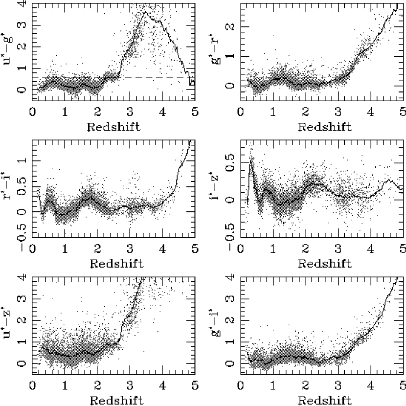
Figure 2: Colors of all 5803 SDSS quasars in our initial sample (grey points). The black lines show the median colors as a function of redshift. The dashed black line in the upper left hand panel is at $u^{*}-g^{*}=0.6$, which might be used as a dividing line between “red” and normal quasars. Note how the use of such a criterion produces a heterogeneous sample as a result of color changes as a function of redshift produced by emission and absorption features. A quasar with $u^{*}-g^{*}=0.6$ can be perfectly normal (if somewhat optically steep) at $z=0.6$, dust reddened at $z=1.2.$, or appear red because of Ly$\alpha$ forest absorption at $z\gtrsim 3$.

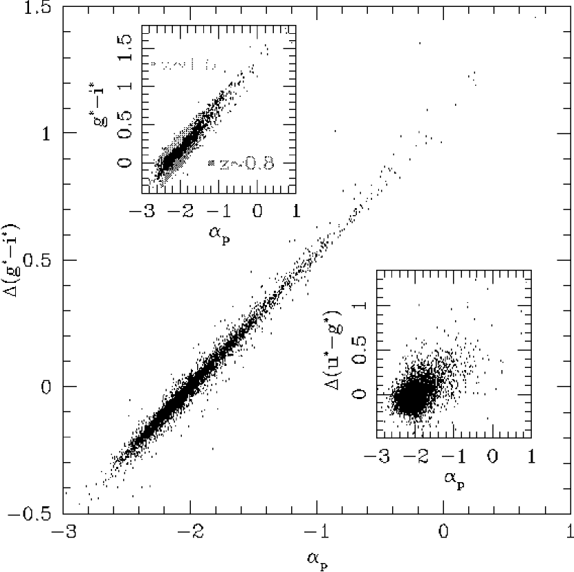
Figure 5: Relative $g^{*}-i^{*}$ colors versus photometric spectral index, $\alpha_{p}$. Upper Left Inset: Observed $g^{*}-i^{*}$ colors versus $\alpha_{p}$. The correlation between $g^{*}-i^{*}$ and $\alpha_{p}$ is not nearly as tight as for $\Delta(g^{*}-i^{*})$ because of redshift effects. Lower Right Inset: Relative $u^{*}-g^{*}$ colors versus $\alpha_{p}$, which shows that the relative $u^{*}-g^{*}$ colors are not a good surrogate for $\alpha_{p}$.

Red quasars are typically searched for using a simple color cut in the observed frame, such as $B-K\gtrsim 5$. In the upper left hand panel of Figure 2 we illustrate such an observed frame color cut (specfically, $u^{*}-g^{*}=0.6$). Although such a criterion does indeed select quasars that are apparently red, it fails to distinguish between four possible cases: (1) that the quasar has an intrinsically red power-law continuum (i.e., is intrinsically optically steep), (2) that the quasar is reddened by dust extinction, (3) that the quasar has excess synchrotron emission, and (4) that the redshift of the quasar is such that the quasar appears to be redder than normal because of strong emission or absorption in one of the bands (e.g., Ly$\alpha$ emission, absorption by the Ly$\alpha$ forest, or BAL troughs). A further example is that of Figure 5 of Barkhouse & Hall (2001) in which they demonstrate that while using $J-K>2.0$ as a color-cut may well select dust reddened quasars, it also selects perfectly normal, if somewhat optically steep, quasars with $z<0.5$. Thus it is perhaps not unexpected that follow-up X-ray observations of such a sample of “red” quasars (Wilkes et al. 2002) finds heterogeneous X-ray properties among red quasars selected in this manner.

There are similar problems with defining red quasars according to spectral indices. For example Gregg et al. (2002), suggest $\alpha<-1$ ($f_{\nu}\propto\nu^{\alpha}$) as an appropriate definition of a red quasar. The problem with this approach is that most spectra do not have enough wavelength coverage for redshift-independent spectral index determination. Vanden Berk et al. (2001) found that there were good continuum windows only at $\sim 1450\,{\rm\AA}$ and $\sim 4000\,{\rm\AA}$; most other commonly used windows are contaminated by Fe II emission. These wavelength regions are only seen simultaneously at $1.30\leq z\leq 1.62$ even in the SDSS spectra, which have broader wavelength coverage than do most other optical quasar studies. Furthermore, the optical spectral index of quasars is a function of the continuum windows used, and therefore depends on redshift (see, e.g., Vanden Berk et al. 2001; Schneider et al. 2002; Pentericci et al. 2003). Finally, using the spectral index can fail to distinguish between quasars that are intrinsically optically steep and quasars that are dust reddened. Dust reddened quasars will have spectral curvature that a simple power-law fit will be unable to characterize.

Observed-color selection is clearly necessary when initiating a follow-up campaign when the redshifts are not yet known. However, interpretation of results from red quasar samples requires the construction of good statistical samples that are independent of redshift. Thus, it is clear that it would be very useful to have a definition for a “red” quasar that takes redshift into account. In particular, we desire a simple but effective selection criterion that depends only on the SDSS photometry (given a redshift), yet correlates strongly with the overall optical/UV spectral energy distribution (SED) of quasars independent of the effect of emission lines. We will show that statistically significant differences in the optical/UV continua of quasars are reflected in their relative colors (the colors referenced to the median color at a given redshift; see below). We also demonstrate these relative colors can be used to distinguish between intrinsically optically steep quasars and dust reddened quasars.

3.2 Rest Frame Selection Using Relative Colors

Rather than determining the continuum color of our quasars by measuring a spectral index from each spectrum, we determine the underlying continuum color by subtracting the median colors of quasars at the redshift of each quasar from the measured colors of each quasar; we will refer to this difference as a relative color (Richards et al. 2001). Figure 2 shows the measured and median colors as a function of redshift in bins of $\Delta z=0.01$ for the SDSS quasars in our sample. As shown by Richards et al. (2001), the features in the color-redshift diagrams can be understood as being due to emission lines moving in and out of the filters. For redshifts between $z=0.6$ and $z=2.2$, we expect the colors of quasars to be dominated by their power law continua and emission lines (as opposed to light from the host galaxy for $z<0.6$ and Ly$\alpha$ forest absorption for $z>2.2$). We also chose to include quasars with $0.3<z<0.6$ so that we sampled both H$\alpha$ and H$\beta$ (in an attempt to study the Balmer decrement); however, in the end, the H$\alpha$ line was too poorly sampled to measure Balmer decrements.

Figure 3 depicts the distributions of the relative colors. The gray points give the individual relative colors as a function of redshift; see Richards et al. (2001) for similar plots as a function of apparent and absolute magnitude. There are no trends in $\Delta(g^{*}-i^{*})$ with position on the sky or Schlegel et al. (1998) Galactic reddening. Furthermore, these color distributions are not predominantly due to photometric errors; the distributions are formally resolved. For example, the FWHM of the $\Delta(r^{*}-i^{*})$ distribution is $\sim 0.2$ and even at $i^{*}\sim 19$ the photometric error in $r^{*}-i^{*}$ is typically only $\sim 0.025$ (FWHM $\sim 0.06$). As a result, we can meaningfully distinguish between blue (optically flat) and red (optically steep) quasars.

As we shall discuss below, from Figure 3 it is quite clear that there is a tail of red quasars which is particularly pronounced in colors involving the $u$ or $g$ filters. (This tail was previously seen in a smaller SDSS sample by Richards et al. 2001.) This tail indicates that the scatter in the colors of quasars is not a simple Gaussian distribution around the median color as can be seen in the lower right hand panel of Figure 3 where we show that a Gaussian distribution (dotted line) can be made to match the blue extent of the distribution, but not the red.

3.3 Photometric Spectral Indices

To determine the overall optical/UV SEDs of our quasars, we fit a power-law to the five SDSS photometric data points in a manner similar to that described by Whiting, Webster, & Francis (2001). Instead of using the observed photometric data points, which will deviate from the underlying power-law continuum because of emission and absorption features, we make use of the relative colors. First, we normalize all of the quasars to have the same apparent $i$ band magnitude since we are only interested in the slope and shape of the continuum. Then we compute the other relative magnitudes from the relative colors. In essence, we have applied a $k$-correction for the emission lines. To determine the spectral index from the relative magnitudes, $m_{rel}$, we utilized the error-weighted linear least-squares fitting routine from Press et al. (1992) and solved for what we refer to as the photometric spectral index, $\alpha_{p}$, according to

$$-0.4\times m_{rel}=\alpha_{p}\log\lambda+C.$$ (1)

using the original magnitude errors as measured in each band and effective wavelengths of 3541, 4653, 6147, 7461, and $8904\,{\rm\AA}$ in $ugriz$ (appropriate for a power-law continuum with $\alpha_{\lambda}=-1.5$ and $f_{\lambda}\propto\lambda^{\alpha}$). By subtracting the median quasar color from all the observed colors, we have essentially defined the relative magnitudes such that the median quasar will now have $f_{\lambda}\propto\lambda^{-2}$ (i.e., $\alpha_{\nu}\equiv 0$).

The solid line in the left panel of Figure 4 shows the resulting distribution of photometric spectral indices, while the dashed line shows the spectral index distributions derived from fitting a power-law to the observed magnitudes in a manner similar to Whiting et al. (2001). The mean offset between the distributions is irrelevant; it merely arises because the relative colors are defined to have a median of $\alpha_{p}=-2$. The right panel of Figure 4 shows the difference between photometric spectral indices using relative magnitudes and observed magnitudes as a function of redshift. Even though both indices recover the tail of red quasars, it is clear that failure to correct for redshift dependent color effects can lead to erroneous photometric spectral indices, where the errors result from not accounting for emission and absorption features (especially the small blue bump) and are systematic with redshift.

3.4 Using Relative Colors To Define Color Samples

Having determined the broad-band SEDs of our quasars, we now ask if we can find a cut (or cuts) using relative colors that can serve as a surrogate for the procedure of finding the photometric spectral index. Surprisingly, the relative $u^{*}-g^{*}$ color, $\Delta(u^{*}-g^{*})$, is not a very good discriminator despite the large spread in that distribution (see the lower right inset of Fig. 5). The observed colors also do not serve as an adequate surrogate for spectral index. The upper left-hand panel of Figure 5 shows that observed $g^{*}-i^{*}$ indeed is correlated with spectral index, but is broadened by redshift effects. For example, a $z=1.5$ quasar with $g^{*}-i^{*}=0.2$ predicts a much bluer (flatter) spectral index than a $z=0.8$ quasar with the same observed color. On the other hand, both the relative colors $\Delta(g^{*}-r^{*})$ and $\Delta(r^{*}-i^{*})$ correlate well with the photometric spectral index and have much less scatter than the observed colors. The combination of the two, $\Delta(g^{*}-i^{*})$, is an excellent redshift-independent surrogate for the photometric spectral index at $z<2.2$ as can be seen in the main panel of Figure 5.

The quantity $\Delta(g^{*}-i^{*})$ can also be used to distinguish between quasars in the red tail and optically steep quasars (at least in a statistical sense). Figure 3 shows that the distribution of relative $r^{*}-i^{*}$ and $i^{*}-z^{*}$ colors is roughly Gaussian and symmetric. If the distribution of colors were purely the result of a roughly Gaussian distribution of power-law spectral indices, the distributions would be similarly Gaussian and symmetric for the other relative colors. However, as we have already mentioned, the other colors, including $\Delta(g^{*}-i^{*})$, show a distinctive asymmetric tail to the red (as highlighted by excess above that of a Gaussian distribution [dotted line] in the lower right hand panel). The objects in this tail are not consistent with an optically steep power-law continuum. This behavior is characteristic of dust reddening, which gives rise to a curved SED.

Based upon the above discussion, we group our sample of quasars into color classes based upon the relative $g^{*}-i^{*}$ color. We begin by isolating the quasars in the red tail of the color distribution, which we presume to be reddened by dust. The definition of such quasars must address the fact that although power-laws are redshift invariant, dust reddened power-laws are not (at least for typical dust extinction curves). Dust-reddened quasars at higher redshift will have redder colors since a given set of filters will sample shorter rest wavelengths, which are more affected by reddening. Therefore, since we believe dust reddening is largely responsible for this population, we must use redshift dependent criteria to select them consistently.

Figure 3 shows no trend of $\Delta(g^{*}-i^{*})$ with redshift. Part of the reason why no trend is seen is that reddened quasars with higher redshifts (which sample bluer rest wavelengths) can be extincted enough that they drop out of the sample, whereas lower redshift quasars with similarly large reddenings will not. If we impose a cut in absolute magnitude ($M_{i^{*}}<-25.61$) such that the least luminous quasars could be seen at all redshifts in our sample, we do see such a redshift trend. This trend is shown in Figure 6, where the $\Delta(g^{*}-i^{*})$ colors of less luminous quasars are shown by points and more luminous quasars by the open squares. The dashed lines show the expected change in color as a function of redshift for an SMC-type reddening law (Prevot et al. 1984; Pei 1992) with $E(B-V)=0.04,0.12,0.20$ (from left to right, and shifted to the red by $0.20$ magnitudes; see caption and next paragraph). In our volume-limited sample (open squares), quasars at higher redshifts are redder, as expected in a dust reddening scenario. There are simply very few low-redshift quasars in our sample area which are intrinsically luminous enough to remain in our sample once they are extincted by an amount corresponding to a reddening of $\Delta(g^{*}-i^{*})\gtrsim 0.5$ at $z\lesssim 1.5$.

As a result of this redshift dependence, we define a dust reddened quasar to be any quasar that is redder than $\Delta(g^{*}-i^{*})=0.2$ by the redshift dependent correction for $E(B-V)=0.04$ (using the SMC reddening law given above), see Table 1. That is, all our putative dust reddened quasars have colors redder than a quasar whose intrinsic power-law continuum slope gives it a color of $\Delta(g^{*}-i^{*})=0.2$ and that is also dust reddened by $E(B-V)=0.04$. Our choice of $E(B-V)=0.04$ is somewhat arbitrary, but it is effective in defining a sample of quasars with color distinct from the general population. In practice, this yields a minimum value of $\Delta(g^{*}-i^{*})\sim 0.3$ for the lowest redshift quasars in our dust reddened sample (see Fig. 6).

For the sake of our analysis, we construct a restricted sample of dust reddened quasars by imposing an upper limit to how red they can be (see Table 1) since we are most sensitive to redder quasars at lower redshifts and we would like our criterion to be consistent as a function of redshift. We exclude objects that are redder than $\Delta(g^{*}-i^{*})=0.2$ by more than $E(B-V)=0.12$ (as a function of redshift) since our completeness drops rapidly for even more heavily reddened quasars. This restriction means that our restricted dust reddened sample excludes the most heavily reddened and absorbed quasars. We will also examine a subsample that includes all of these quasars, but even this sample will not include quasars of the type discussed in Hall et al. (2002a) since those quasars were all identified by eye and not by the automated algorithm on which we have relied for our sample. Such quasars are also of significant interest and will be discussed in future papers. Of the 4576 quasars in our sample, 273 (6.0$\pm$0.4%) are redder than the $E(B-V)=0.04$ cut and can be considered to be dust reddened; 211 (4.6$\pm$0.3%) also meet the $E(B-V)=0.12$ upper limit condition that we impose for the sake of uniformity and will constitute our restricted dust reddened sample in the following sections. (The uncertainties on the percentages above are statistical only, and neglect the effects of systematic errors.)

Our redshift dependent definition of a dust reddened quasar technically introduces a bias into the sample in that we have defined the cut with the explicit assumption of dust reddening. Clearly it would be better to define dust reddened quasars in terms of their rest-frame colors, but we cannot do so without interpolating (and extrapolating) our data. It could be argued that our definition weakens our hypothesis that the sample is indeed dust reddened. For example, the non-LTE accretion disk models of Hubeny et al. (2000) predict quasi-thermal spectra with significant intrinsic curvature in the rest-frame UV; such objects could fall within our dust reddened definition. In their model, lower luminosity objects also tend to have greater curvature (their Figure 13). This could explain why the $M_{i^{*}}\geq-25.61$ objects in our Figure 6 extend to redder colors at $z\lesssim 1.5$ than do the $M_{i^{*}}\leq-25.61$ objects. However, their model does not explain why the $M_{i^{*}}\leq-25.61$ objects extend to redder colors at $z\gtrsim 1.5$ than at $z\lesssim 1.5$. Furthermore, we would argue that the photometric properties of the sample (Fig. 3) support our conclusion that the reddest quasars in our sample are likely to be dust reddened — independent of our choice of definition.

Once we have isolated quasars that are probably dust reddened, it is easy to divide the remainder of the objects into further color classes. Quasars with $\Delta(g^{*}-i^{*})$ colors that are not in the red tail of the distribution, $\Delta(g^{*}-i^{*})\gtrsim 0.3$, are considered to be “normal” — their range of colors is consistent with that caused by a distribution of power-law continua. We do not impose a redshift dependent criterion to break the normal quasars into color subclasses; we merely subdivide them into color classes along lines of constant $\Delta(g^{*}-i^{*})$. See Table 1 and below for the definition of the four normal color quasar samples that we will use in our analysis.

4 Composite Spectra

4.1 Composite Spectra Construction

We now create composite spectra as a function of relative color (optical continuum slope) to study the dependence of spectral properties on color in the ensemble average. The composites are constructed in the same fashion as the Vanden Berk et al. (2001) SDSS quasar composite, using the same code. In detail, the quasars are sorted by their cataloged redshifts, shifted to their rest frame wavelengths, rebinned to a common wavelength scale, scaled by the overlap of the preceding average spectrum, and weighted by the inverse of the variance. The geometric mean of the spectra is used, which preserves input power-law slopes [and $E(B-V)$ values, if the extinction curve is the same in all objects].

Four samples of “normal” color quasars are created as a function of color by separating all quasars with $\Delta(g^{*}-i^{*})\leq 0.3$ into quartiles in $\Delta(g^{*}-i^{*})$; see Table 1. Each quartile contains 1053 quasars. Next, we examine the redshift and absolute magnitude distributions of each quartile in bins of $\Delta M_{i}=0.5$ and $\Delta z=0.2$. We restrict the number of quasars in each redshift-magnitude bin to the smallest number in that bin for any of the four quartiles. Each quartile then has only 770 quasars, but now the quartiles have roughly the same redshift and absolute magnitude distribution, which allows us to compare differences between the samples without having to worry that they are caused by redshift or luminosity effects. Table 1 gives the number of quasars in each of the subsamples, the $\Delta(g^{*}-i^{*})$ color limits, the spectral index of the composite spectra (see below), and the number and percentage of FIRST-detected radio sources.

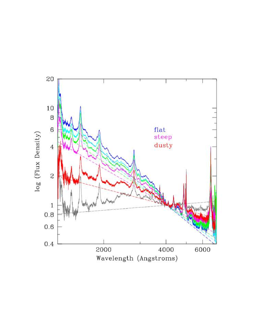
Figure 7: Composite spectra as a function of $\Delta(g^{*}-i^{*})$, normalized at $4040\,{\rm\AA}$. The blue, cyan, green, and magenta spectra are the four normal quasar composite spectra that have similar absolute magnitude and redshift distributions (composites 1-4). The red spectrum is the dust reddened composite (composite 5); it has a different absolute magnitude and redshift distribution from the other four spectra. Composite 5 has significant curvature. It is not well fit by a power-law at $2200\,{\rm\AA}$ or for $\lambda\gtrsim 5000\,{\rm\AA}$. The gray spectrum is a composite (number 6) of all of the dust reddened quasars that were too red to be included in the primary dust reddened composite; see text.

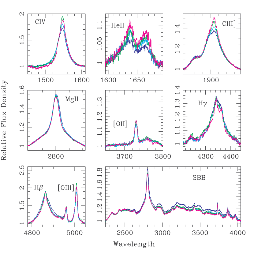
Figure 8: Expanded emission line regions from Figure 7 (composites 1-4). “SBB” refers to the $3000\,{\rm\AA}$ (or small blue) bump. The color scheme is the same as for Figure 7. The spectra are normalized such that their continua agree at the edges of the panels.

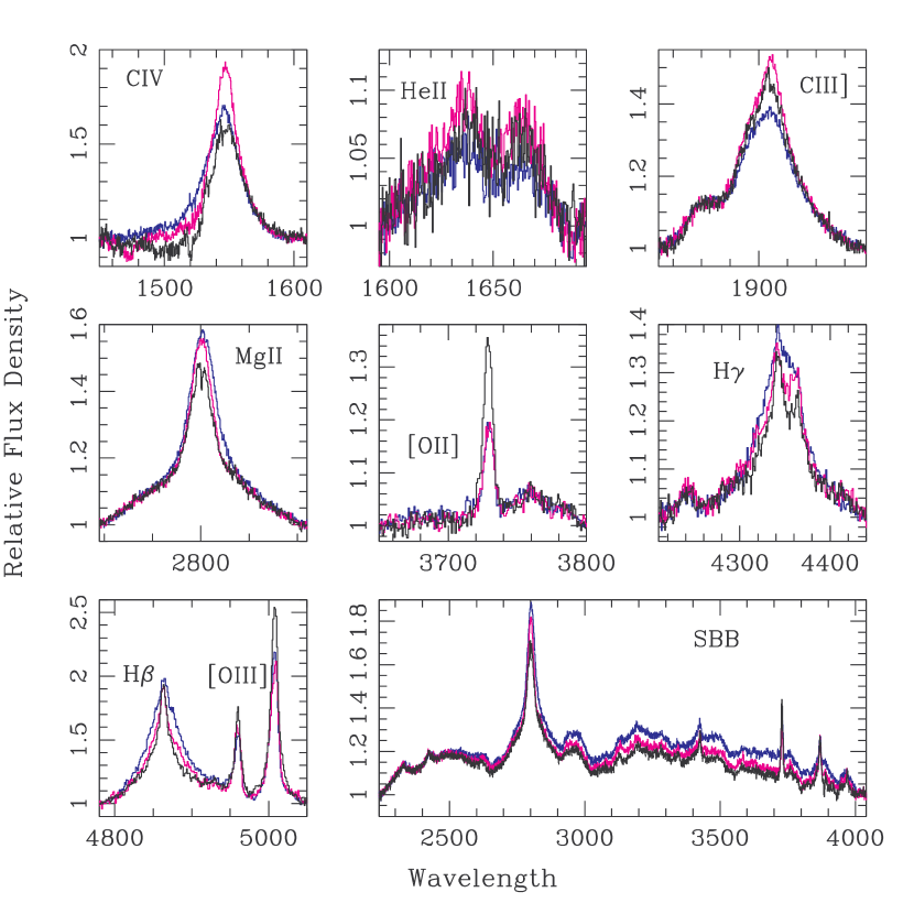
Figure 9: Expanded emission line regions of the bluest and reddest absolute magnitude and redshift normalized composite spectra (composites 1n and 4n, cyan and magenta, respectively), and the absolute magnitude and redshift normalized dust reddened composite spectrum (composite 5n, black). The spectra are normalized such that their continua agree at the edges of the panels.

We create composite spectra for each of these four samples (hereafter “composites 1-4”); these are shown in blue, cyan, green and magenta in Figure 7. The spectral indices (as measured from $1450\,{\rm\AA}$ to $4040\,{\rm\AA}$) are $\alpha_{\nu}=$ $-0.25$, $-0.41$, $-0.54$, and $-0.76$, respectively. These values are less reliable with increasing redness due to the presence of broad absorption line troughs in the reddest samples (see the C IV emission line regions in the upper left-hand panels of Fig. 8 and Fig. 9) and any possible curvature induced by dust extinction. That our photometrically defined color samples yield composite spectra with power-law continua in the same sense as their input colors testifies to the quality of the SDSS’s spectrophotometry.

We also create a composite dust reddened quasar spectrum (hereafter “composite 5”) by combining all 211 spectra that meet the restricted definition given above. The dust reddened spectrum is shown in red in Figure 7. A single power-law is a poor fit to this spectrum, as can be seen by examining the spectrum at $\lambda\sim 2200\,{\rm\AA}$ and $\lambda\gtrsim 5000\,{\rm\AA}$. In addition, we present a composite spectrum of the 62 quasars that are redder than the upper limit on the dust reddened composite that we imposed above; this composite (hereafter “composite 6”) is shown in gray in Figure 7. The quasars that contribute to the dust reddened composite (composite 5) have a different distribution in $M_{i}$ vs. $z$ space than the quasars in the normal color composites that we defined above: on average, the spectra are $0.55$ mag fainter. Thus, we have also created subsamples of the four normal quasar samples and the dust reddened sample such that the four new normal color samples and the new dust reddened sample all have the same distribution in $M_{i}$ vs. $z$ space; see Table 1. These five new composite spectra (hereafter “composites 1n-5n”) have 185 quasars each and are similar to the original composites, but have lower signal-to-noise, so we have not shown them in full (but see Fig. 9).

4.2 Composite Spectra Analysis

In addition to the change in the power-law spectral index with $\Delta(g^{*}-i^{*})$, some interesting changes occur to the emission line features. Here we point out some of the more obvious trends that will be important for our later discussion. The major emission line regions of interest are shown in Figures 8 and 9. These spectra have been normalized using local continuum windows at the edges of the plots. See Table 2 for the equivalent widths of the major emission lines in the color composite spectra. Below we comment on each of the panels in these figures. We begin by examining the four normal color composite spectra (composites 1-4; Fig. 8) that are normalized to have the same redshift and absolute magnitude distribution.

C IV — There is no clear systematic trend in C IV height or width with color, although the redder spectra do seem to have higher peaks and slightly wider profiles. There is, however, a clear trend in the existence of BAL-like absorption blueward of the C IV emission line; the reddest quasars (composite 4) clearly have more absorption on average, although the absorption feature is diluted because of averaging with nonBALQSOs in the composite. There also appears to be a slight blueshift of the line (as seen in the red wing of the line) with bluer colors; see also Richards et al. (2002b).

He II — The strength of He II $\lambda 1640\,{\rm\AA}$ grows with increasing redness. The same is true for the O III]/Al II/Fe II blend just redward of the He II line.

C III] — There is a very clear systematic trend of increasing C III] $\lambda 1909\,{\rm\AA}$ height with increasing redness. The nearby Al III $\lambda 1857\,{\rm\AA}$ and Si III] $\lambda 1892\,{\rm\AA}$ lines do not seem to show any change with color. The Fe III$\lambda\lambda$1895,1914,1926 Å complex also affects this wavelength region, but the profile change cannot be explained entirely by changes in the Fe III strength since the four composites agree well redward of the C III] peak.

Mg II — Mg II shows a weak, but clear trend towards weaker lines with increasing redness. There is also a slight ($\sim 150\,{\rm km\,s^{-1}}$), but systematic shift of the line peak to the blue with increasing redness. Interestingly, this shift has a color trend that is opposite to that of C IV.

[O II] — The two reddest composites have somewhat stronger [O II] $3727$ than the two bluest composites (see Table 2); however, the differences are relatively small.

$H\gamma$ — The $H\gamma$ line (which is blended with [O III] $\lambda$4363) is somewhat narrower in the reddest composite spectrum.

$H\beta$ — A systematic narrowing of the $H\beta$ line is seen with increasing redness. No systematic trend is seen for the [O III] lines.

$3000\,{\rm\AA}$ bump — There exists a very clear trend towards a weaker $3000\,{\rm\AA}$ (small blue) bump with increasing redness. This trend is consistent with that seen by Baker & Hunstead (1995) for a sample of radio-selected quasars, where both trends were a function of increasing radio core-to-lobe flux density ratio $R$ — that is, orientation. This issue is discussed further in the next section.

Unfortunately, we are not able to investigate $H\alpha$ (or the Balmer decrement) since there are not enough quasars in each sample at this wavelength.

The above trends are all with respect to the normal color composite spectra. Also of interest is how the dust reddened composite spectrum fits into these trends. Figure 9 depicts the absolute magnitude and redshift normalized dust reddened composite (5n) along with composites 1n and 4n. For these composites, we find the following trends. C IV is quite weak in the dust reddened spectrum; both the emission line and the continuum just blueward of the emission line are absorbed. The C III] emission line appears intermediate in strength between the bluest and reddest composites. The Mg II emission line is weaker than the other color composites and shows signs of intrinsic absorption with $z_{\rm abs}\sim z_{\rm em}$. [O II] $3727$ is much stronger in the dust reddened spectrum than in all of the other color composites. Both $H\beta$ and $H\gamma$ are noticeably narrower in the dust reddened composite spectrum. [O III] is considerably stronger in the dust reddened spectrum. The $3000\,{\rm\AA}$ bump in the dust reddened spectrum is the weakest of all of the composites, continuing the trend of a weaker feature with increased redness.

5 Discussion

5.1 Red vs. Reddened

The shape of our putative dust reddened composite spectrum reveals something fundamental about its nature. The two primary causes of red continua in the optical were discussed in detail by Francis et al. (2000). In their investigation of a sample of radio-detected quasars they showed that if quasars are redder because of the addition of a synchrotron turnover, then we expect them to be redder at red wavelengths than at blue wavelengths (i.e., they will have “u” shaped continua). On the other hand, if the quasars are redder at blue wavelengths, then they are reddened by dust extinction (i.e., they will have “n” shaped continua). Figures  3 and 7 show that our (mostly radio-quiet) quasars are are clearly redder at blue wavelengths than at red wavelengths — “n” shaped — and we conclude that these red quasars are redder in a way that is consistent with dust extinction and inconsistent with synchrotron emission. We have not fully investigated the nature of red radio-loud quasars separately since they are few in our sample, but their color distribution (see the two dashed histograms in Fig. 3) suggests that dust reddening is at work in radio-detected quasars as well as radio-undetected ones.

We can then ask how red our dust reddened composite is relative to the normal color composites. Using an SMC-like reddening law with dust local to the quasar, we find that the normal color composites (1n to 4n) need to be reddened by approximately $E(B-V)=0.135,0.11,0.10,{\rm and}\,0.07$, respectively from blue to red to fit the dust reddened composite spectrum (5n). A composite spectrum that includes all of the quasars in samples 1n, 2n, 3n and 4n requires $E(B-V)\simeq 0.11$ to fit composite 5n. These results are not surprising given our dust reddened quasar definition, but the relative values are still of interest.

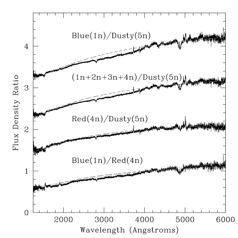
Figure 10: Composite spectra ratios (black lines). The bottom ratio spectrum is normalized to unity at $4040\,{\rm\AA}$; the top three spectra are each shifted upwards from the preceding spectrum by one unit in the flux density ratio. For each ratio we overplot an SMC reddening curve (gray dashed lines) with $E(B-V)=0.135,0.11,0.07$, and $0.035$ from top to bottom, respectively. For the ratio of the bluest to reddest (optically flattest and steepest; bottom panel) power-law composites we also overplot a curve (dotted gray line) showing a change in spectral index of $\Delta\alpha=0.45$.

Figure 10 displays the ratios of composites 1n to 5n; the average of 1n, 2n, 3n, and 4n to 5n; 4n to 5n; and 1n to 4n, respectively from top to bottom. Overplotted in gray dashed lines are SMC reddening curves with $E(B-V)$ values of 0.135, 0.11, 0.07 and 0.035, respectively. These reddening values result in good matches to the dust reddened composite (5n) at both $1700\,{\rm\AA}$ and $4040\,{\rm\AA}$, but they overpredict the flux between these wavelengths and underpredict the flux shortward of C IV. This discrepancy between these wavelengths is most likely the result of differences in the strength of the Balmer continuum between the composites. If we modeled these Balmer continuum differences, the resulting SMC reddening curves would trace the overall continuum differences much more closely. Similar results are found when using a simple $1/\lambda$ reddening law as given by Francis et al. (2000). Reddening the normal color composites with the shallower LMC reddening curve produces only marginally better fits to the dust reddened composite spectrum.

The issue of the color differences between the normal composites is somewhat more complicated. To help address this question, in the bottom panel of Figure 10, we overplot a curve (dotted gray line) showing a difference in spectral index of $\Delta\alpha=0.45$ on the ratio of the bluest to the reddest of the power-law composites. Comparing this curve to the curve produced by pure SMC reddening (dashed gray line) suggests that it is likely that dust reddening plays some role in the color differences between composites 1-4, since the ratio spectrum has slightly more curvature than the spectral index difference curve. Indeed, we will argue in § 5.3 that the C IV emission line shape as a function of color suggests that some intrinsically blue (optically flat) quasars are being reddened by dust into the redder (steeper) color bins. At the same time, reddening alone cannot be the cause of the significant trends in emission line properties from composite 1 to composite 4. Either the emission lines are responding directly to differences in the ionizing continuum, or both the optical SED and the emission lines are changing as a function of some other property (such as orientation or accretion rate). As a result, we suggest that the color changes between composites 1 through 4 are dominated by changes in the intrinsic continuum rather than by dust reddening (see § 5.3).

Finally, these ratio spectra in Figure 10 also highlight some of the changes in the emission line regions that we discussed earlier. One new result from this presentation is that the narrow component of H$\beta$ seems to be relatively constant while the broad component is changing (as can be seen by the inflection in the H$\beta$ residual profile).

5.2 BALQSOs and Reddening

It has been noted by numerous authors that BALQSOs, especially LoBALs, are redder than the average quasar (Sprayberry & Foltz 1992; ; Yamamoto & Vansevičius 1999; Becker et al. 2000; Najita, Dey, & Brotherton 2000; Brotherton et al. 2001; Hall et al. 2002a; Reichard et al. 2003), likely as a result of extinction by dust. The reddest of our four color composites and the dust reddened composite spectrum show considerable absorption blueward of C IV, in agreement with this result.

An interesting issue is the BALQSO fraction as a function of optical color; we explore this question using a well-defined BALQSO catalog (Reichard et al. 2003) from the SDSS Early Data Release (EDR; Stoughton et al. 2002). First, we consider only those quasars that would have been selected by the Richards et al. (2002a) algorithm since the EDR quasar sample was not selected with one uniform algorithm. Second, we consider only quasars with $1.7\leq z\leq 2.2$ so that the sample is restricted to those quasars for which a BALQSO classification was made using spectra of the C IV absorption region. Finally, we divide the quasars into four equal bins of normal color quasars (with 434 quasars in each bin) in the same manner as for our primary sample, and we also define an EDR dust reddened sample with 96 quasars. We find that from bluest to reddest (optically flattest to steepest), the BALQSO fractions are $3.4\pm 1.5$%, $6.3\pm 2.3$%, $10.3\pm 2.7$%, and $18.1\pm 3.5$%. The BALQSO fraction among EDR dust reddened quasars is is $20.0\pm 8.9$%, after restricting the samples such that they have the same absolute magnitude and redshift distributions.

Thus, in agreement with the work cited above, we find that the presence of BAL troughs and reddening are highly correlated. It is unclear to us whether the BAL material always reddens the intrinsic quasar spectrum, or if reddened quasars are more likely to be BALQSOs, but there is little doubt that BALQSOs are indeed reddened in a manner that is consistent with dust extinction. If BALQSOs suffer from dust extinction, then the fractions as a function of color given above are not the intrinsic fractions. That is, BAL troughs may be just as common in intrinsically blue (optically flat) quasars as in intrinsically red (optically steep) quasars if dust extinction skews the observed distribution of colors to the red.

In this analysis, we also must be careful about how any broad absorption troughs affect the colors of BALQSOs since the C IV trough will often fall within the $g$ band. For the majority of BALQSOs the change in color due to reddening in the $g$-band will dominate over the change in color due to an absorption trough in the $g$-band, as can be seen from the following argument. The standard measure of C IV BAL strength is the “balnicity” index, which is sensitive to flux decrements of 10% or more over a span of $25,000\,{\rm km\,s^{-1}}$ (from the peak of Si IV to the peak of C IV, or roughly $450\,{\rm\AA}$ at $z=2$) (Weymann et al. 1991). On the other hand, a $z=2$ quasar with $E(B-V)$ of only $0.03$ has a flux decrement across the entire $g$-band of 14% (relative to the $i$-band, and assuming SMC-like intrinsic reddening). Since the $g$-band has an effective width that is more than twice the wavelength range considered when calculating balnicities and since BAL troughs rarely span as much as $25,000\,{\rm km\,s^{-1}}$ (Reichard et al. 2003), the effective absorption due to reddening completely dominates that caused by absorption troughs. Our use of relative $g^{*}-i^{*}$ colors as a tracer of continuum color thus is valid for the vast majority of BALQSOs, failing only for FeLoBALs and for LoBALs with very extensive absorption (Hall et al. 2002a).

5.3 Emission Line Trends with Color

Many of the emission line trends with color discussed in § 4.2 can be related to the principal component analysis (PCA) of quasars, which has become popular in recent years (Boroson & Green 1992; Sulentic et al. 2002). The basic idea of PCA is to describe the data by orthogonal eigenvectors and to study the resulting distribution of eigenvalues to learn something about the underlying physics of quasars. Of particular interest are the correlations with the first eigenvector as found by Boroson & Green (1992) and summarized by Brotherton & Francis (1999).

One of the key emission lines used in eigenvector analysis is [O III] (see Brotherton & Francis 1999, and references therein). In our sample, little difference is seen in [O II] and [O III] among the normal color composites; however, both of these lines are significantly stronger in the dust reddened composite. This result suggests that optically steep quasars are not produced exclusively by dust reddening, but that the dust reddened spectrum is affected since the increase in line strength is larger at [O II] $\lambda 3727\,{\rm\AA}$ than at [O III] $\lambda 5007\,{\rm\AA}$ — as expected in a simple dust reddening scenario where dust affects the continuum and broad emission line region (BELR), but not the narrow emission line region .

We can test the consistency of this scenario by comparing the [O II] and [O III] EWs predicted for a reddened normal quasar with the observed EWs of the dust reddened composite. The [O III]$\lambda$5007 EW for the dust reddened quasars is 18.97 Å, while the average for normal quasars (composites 1n-4n) is 14.15 Å. Assuming the continuum is extincted but the narrow-line region is not, to match this difference requires $E(B-V)=0.10$ with the SMC extinction curve, in good agreement with the extinction required to best match the normal quasar composite to the dust reddened composite. However, the [O II]$\lambda$3727 EW for dust reddened quasars is 2.81 Å (after correcting for the 5% weaker Balmer decrement in the dust reddened composite at 3727 Å), while the average for normal quasars is 1.39 Å, and to match this difference requires $E(B-V)=0.17$.

This discrepancy could be explained if dust reddened quasars have stronger [O II] emission than normal quasars. Croom et al. (2002) suggest that a significant portion of the [O II] flux in quasars arises from the host galaxy. If true, stronger [O II] in dust reddened quasars might be expected, as galaxies with significant dust content are also likely to have significant star formation. Another possibility is that [O III] emission is less isotropic (or more anisotropic) than that of [O II]. Such anisotropy could occur if the higher-ionization [O III]-emitting region extended to small enough radii to be partially obscured by the dust which reddens the quasars (e.g., a dusty torus viewed at high inclination). This latter geometry has been suggested for radio-loud quasars (Hes, Barthel, & Fosbury 1996) though it may not apply to radio-quiet quasars (Kuraszkiewicz et al. 2000). Note that in this latter case there would have to be a range of reddenings across the sightline(s) to the continuum source (Hines & Wills 1995) to explain why the continuum appears reddened by only $E(B-V)=0.1$, instead of $E(B-V)=0.17$.

Boroson & Green (1992) also noted that there is an anti-correlation between the strengths of [O III] and Fe II. If the small blue bump is dominated by Fe II emission, the small blue bump being weak in dust reddened quasars when [O III] is strong would be consistent with this anti-correlation. However, as can be seen in the ratio spectra in Figure 10, the difference between composite 1n and the dust reddened composite (5n) has a minimum near $3500-3700\,{\rm\AA}$, rises steadily towards the blue, and rises more rapidly to the red. This behavior is consistent with this color-dependent component of the small blue bump being dominated by the Balmer continuum as opposed to Fe II and Fe III emission (Wills, Netzer, & Wills 1985).

Although Boroson & Green (1992) argue that their “Eigenvector 1” is independent of orientation, it is interesting to examine these results from an orientation perspective by comparing our results to the results of investigations of radio-loud quasars. Baker & Hunstead (1995) and Baker (1997) argue that radio-loud quasars (RLQs) of increasing lobe dominance are seen through increasing amounts of dust (i.e., RLQs are redder the closer they are to edge-on) and are observed to have weaker small blue bumps. The weaker small blue bump, stronger oxygen lines, and greater EW increase in [O II] than in [O III] seen in our dust reddened composite could be consistent with their argument (but see Kuraszkiewicz et al. 2000). It has also been suggested that an orientation effect would result if $H\beta$ were emitted from a disk-like structure (Wills & Browne 1986; Vestergaard, Wilkes, & Barthel 2000) with broader lines coming from quasars seen more edge-on. Curiously, however, if the change in the width of the Balmer lines is a function of orientation, then our results — narrower lines in objects which are presumably closer to edge-on (optically steep and dust reddened quasars) — conflict with Wills & Browne (1986). These conflicting results may indicate a real difference between the BELRs of radio-loud and radio-quiet quasars. Another possible explanation for the change in width of H$\beta$ with color is a correlation with black hole mass (Vestergaard 2002); perhaps the bluer (flatter) quasars simply have more massive black holes.

In an investigation of the X-ray properties of quasars, Laor et al. (1997) found a correlation between the width of H$\beta$ and the X-ray spectral index in the sense that narrow H$\beta$ corresponds to a soft X-ray dominated spectrum and higher $L/L_{Edd}$ (though it is unclear whether the X-ray SED is due to a soft X-ray excess or an intrinsically steep X-ray spectrum). Given our own results, this finding implies that redder quasars may have steeper X-ray spectral indices or larger soft X-ray excesses. Similarly, we have weak evidence that redder quasars are more likely to be radio sources than the bluer quasars (see Table 1). This result is consistent with Richards et al. (2002b) if redder quasars also have smaller C IV blueshifts (which will require a larger sample to determine). On the other hand, Sulentic et al. (2002) found that it was the radio-quiet quasars that tended to have the narrowest H$\beta$ emission lines and the largest soft X-ray excesses. Clearly more work is needed to understand the X-ray and radio properties as a function of color.

Another particularly interesting dilemma with regard to the emission lines as a function of color involves C IV, He II and C III], all of which are popular lines in eigenvector analyses. Richards et al. (2002b) found that quasars with large C IV blueshifts with respect to Mg II tended to have weaker C IV, He II and C III] emission and also tended to be bluer than quasars with small C IV blueshifts. Similarly, this paper’s color-divided samples also show that the bluest quasars have the weakest C IV, He II, and C III] emission. Richards et al. (2002b) argued that the emission line properties of such quasars were most similar to BALQSOs (or vice versa), whereas in our present work, it is the reddest quasars that are most likely to be BALQSOs. This trend with color for these three emission lines does not seem to extend to the dust reddened sample, which contains the most BALQSOs (see § 5.2). This discrepancy may be reconciled if dust reddened, but intrinsically blue quasars contaminate the redder composites, including the dust reddened composite, and if BALQSOs are drawn from a bluer parent population (Reichard et al. 2003).

5.4 The Fraction of Missing Quasars

We have not formally addressed the question of what fraction of quasars are missed by normal optically-selected samples of quasars because of reddening or because they would be classified as “Type 2” (narrow line only) quasars (e.g., Norman et al. 2002). Estimates for the fraction of optically extincted quasars that are “missing” have ranged as high as 80% for radio-quiet quasars, based on the existence of red radio-loud quasars (Webster et al. 1995). In addition, X-ray surveys estimate that a significant fraction of AGNs are undetected in the optical if obscured AGNs (particularly Type 2 quasars) are the primary contributors to the X-ray background (Mushotzky et al. 2000; Brandt et al. 2000).

Our red quasar sample can be used to reveal something about the population of reddened quasars that might be missed by blue-sensitive flux-limited surveys, but that are recovered by the SDSS. A full characterization of the incompleteness of previous UVX quasar surveys to dust reddened quasars is beyond the scope of this paper. We merely point out that the SDSS must, by definition, be more sensitive to dust reddened quasars simply because the SDSS is flux limited in the $i$-band instead of the $B$-band and because dust extinction is stronger at bluer wavelengths than red. Yet even our sample must be incomplete since despite the SDSS’s sensitivity to red quasars and its $i$-band selection, most quasars that are heavily dust reddened [$E(B-V)\gtrsim 0.5$] will be extincted below the limiting flux of even the SDSS.

Furthermore, our sample is restricted to those objects that were automatically classified as quasars by the SDSS’s spectroscopic pipeline. Quasars that have absent, weak, or very narrow emission lines; or that are extremely reddened, or show strong intrinsic absorption, such as those described by Hall et al. (2002a), are missing from this sample. Examples of extremely reddened quasars are rare, but they carry considerable weight since they are intrinsically luminous and are the only representatives in the SDSS of the population of similarly reddened but less luminous quasars. Thus, they must also be considered when determining the fraction of missing quasars. A full analysis of this issue is beyond the scope of this paper (and data set), but with the data in hand, we can perform some preliminary incompleteness calculations.

We can make a rough estimate of the fraction of missing quasars with $E(B-V)$ values within the limits of detectability by the SDSS. We take $E(B-V)$=0.11 (see §5.1) as representative of the dust reddened quasar population relative to normal quasars. At a representative $z=2$, observed $g$ and $i$ correspond to roughly 1550 Å and 2500 Å in the rest frame. An SMC extinction law with $E(B-V)$=0.11 produces $A_{1550}$=1.43 and $A_{2500}$=0.81 and thus reddens the observed $g^{*}-i^{*}$ color by $\Delta(g^{*}-i^{*})=0.62$. At a given apparent magnitude, for this representative SDSS-detected dust reddened quasar we are sampling the $i$-band luminosity function 0.8 magnitudes brighter than for normal quasars. In the luminosity range of our quasar sample, the 2dF QSO luminosity function (Boyle et al. 2000) shows an increase in the number of quasars of about a factor of 3 per unit magnitude. We must thus correct the number of dust reddened quasars with $\Delta(g^{*}-i^{*})=0.6$ by a factor of 2.5, $\Delta(g^{*}-i^{*})=1.2$ by a factor of 6.25, and so on. There are only 9 dust reddened quasars with $\Delta(g^{*}-i^{*})>0.9$ in our sample which require this factor 6.25 correction (Fig. 6); the remaining 264 dust reddened quasars will have a factor 2.5 correction. Thus, in addition to the 273 dust reddened quasars detected in our SDSS sample, constituting 6% of that sample (4.5% if we restrict the sample to $i^{*}<19.1$), we estimate that there are a further 443 (a further 10%) which would have been included in our SDSS sample if they had not been reddened. This fraction, however, assumes that our quasars have magnitudes near our flux limit and therefore somewhat overestimates the actual fraction of dust reddened quasars that the SDSS might miss. Nevertheless, this estimate, while crude, illustrates the importance of accounting for the reddening of such quasars when studying the full extent of the quasar population.

We can also make more general conclusions about the total AGN population. Specifically, the distribution of colors in our optical data suggests that the hidden X-ray population cannot be due to a continuous distribution of dust reddened, but otherwise normal Type 1 quasars. If the fraction of missing dust reddened Type 1 quasars were near 50%, the $\Delta(r^{*}-i^{*})$ and $\Delta(i^{*}-z^{*})$ color distributions shown in Figure 3 would be skewed to the red. Thus, if the X-ray background is due to obscured AGN, there would either have to be a class of broad-lined quasars whose reddening distribution is disjoint from the distribution that we observe, or the quasars would have to have their broad-line region obscured and thus would be classified as Type 2 quasars (as is generally suspected). In fact, another way of viewing the problem is described by Ivezić et al. (2002) who used FIRST-SDSS matches to show that the SDSS quasar survey is at least 89% complete to broad-lined AGN.

6 Conclusions

We have presented a homogeneously selected sample of 4576 SDSS quasars with $0.3\leq z\leq 2.2$ and $i^{*}<19.9$. The majority of these quasars are well-fit by a power-law continuum with spectral indices ranging from $\alpha_{\nu}=-0.25$ to $\alpha_{\nu}=-0.76$ (optically flat to optically steep). There is also a population of quasars that are red in comparison with even the reddest power-law continuum (optically steep) quasars and that are probably dust reddened. This population is $\simeq 6.0\%$ of the sample, a large fraction of which are likely to be missed by blue-sensitive optical surveys for quasars. A rough correction for incompleteness due to the extinction in this population suggests that the true fraction of dust reddened red quasars to which the SDSS quasar survey would otherwise be sensitive is $\simeq 15\%$.

Among the power-law continuum quasars, optically steep quasars are observed to have stronger emission at C IV, C III], and He II. The strength of the $3000\,{\rm\AA}$ bump is weaker in optically steep quasars than in optically flat quasars. This change in strength appears to be dominated by weakening of Balmer emission rather than iron emission. In addition to weaker Balmer continuum, redder quasars (including the dust reddened ones) have narrower Balmer lines. For the dust reddened quasar sample, we also find that [O II] and [O III] emission have very large equivalent widths.

We also find that BALQSOs appear to be more common among red quasars than among blue quasars and that this color distribution cannot be caused by the absorption troughs themselves. The BALQSO fraction is as high as 20% among the dust reddened quasars and as low as 3.4% in optically flat quasars. However, these fractions fail to account for the possibility that BALQSOs may be systematically reddened by dust and may have an intrinsically bluer parent population.

Further work on both the color distribution of quasars and the population of dust reddened quasars will benefit considerably from the availability of much larger samples of SDSS quasars in the near future, and from the extension of our technique to somewhat higher redshifts. In particular, we will be able to study the very reddest quasars found by the SDSS, which are much redder than those considered herein. We will also be better able to explore the questions of whether the reddening is always due to dust, how often the dust is intervening rather than intrinsic, and what the form of the average reddening law is in both cases.

Figure 1: Left: Completeness for simulated red (optically steep) but unextincted quasars with $\alpha_{\nu}=-1.5\pm 0.3$. Right: Completeness for simulated dust reddened and extincted quasars with $E(B-V)=0.1$ (assuming SMC dust extinction). In both panels, contours are drawn at 10, 25, 50, 75 and 90% completeness, with the 90% completeness contour shown as a dashed line. The shaded region is where there are no objects in the simulations; quasars more luminous than the most luminous of our simulated quasars are clearly even more likely to be detected.

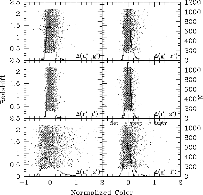
Figure 3: Relative colors of the 4576 quasars with $0.3\leq z\leq 2.2$, $i^{*}<19.9$, and $M_{i^{*}}<-23.0$. The grey points are a scatter plot of the relative colors ($x$-axes) versus the redshift (left hand $y$-axes). The black histogram is a histogram of the number of quasars as a function of relative color; the number in each bin is given by the right-hand $y$-axes. The dashed histograms in the $\Delta(u^{*}-g^{*})$ and $\Delta(i^{*}-z^{*})$ panels show the relative color distribution of radio-detected quasars (binned at half the resolution and multiplied by a factor of 5). The dotted line in the lower right hand panel shows a Gaussian color distribution as fit to the peak and blue wing; note the clear excess of quasars to the red. The top of the $\Delta(g^{*}-i^{*})$ panel shows the progression of optically-flat to optically-steep to dust reddened in our adopted nomenclature.

Figure 4: Left: Histogram of photometric spectral indices computed from the relative magnitudes of each quasar (solid line). The dashed line shows the histogram of spectral indices computed using the observed instead of relative magnitudes. Right: Difference between redshift corrected photometric spectral index and uncorrected photometric spectral index as a function of redshift. The expected difference is $\sim 0.5$; larger values indicate that the uncorrected photometric spectral index is too red.

Figure 6: Redshift versus relative $g^{*}-i^{*}$ color for quasars with $M_{i^{*}}<-25.61$ (open squares) and $M_{i^{*}}\geq-25.61$ (small points). The dotted line shows the effect of SMC-type reddening as a function of redshift with $E(B-V)=0.04$. The dashed lines are for $E(B-V)=0.04$, $0.12$, and $0.2$, respectively, but are shifted redward by 0.2 to match our dust reddened quasar definition. The two thicker dashed lines at $E(B-V)=0.04,0.12$ outline the part of the dust reddened quasar region that we use to create our primary dust reddened composite spectrum.

Table 1: Sample Definitions

Sample	${\rm N_{QSOs}}$	$\Delta(g^{*}-i^{*})_{\rm min}$	$\Delta(g^{*}-i^{*})_{\rm max}$	$\alpha$	Radio
1	770	$-$0.461	$-$0.109	$-$0.25	18/3.0
2	770	$-$0.109	$-$0.032	$-$0.41	32/5.5
3	770	$-$0.031	+0.066	$-$0.54	26/4.4
4	770	+0.066	+0.299	$-$0.76	51/8.7
5	211	$+0.200$	$+0.200$	$\cdots$	$\cdots$
		$+E(B-V)\geq 0.04$	$+E(B-V)\leq 0.12$
6	62	$+0.200$	$\cdots$	$\cdots$	$\cdots$
		$+E(B-V)\geq 0.12$	$\cdots$
1n	185	$-$0.461	$-$0.109	$\cdots$	0/0.0
2n	185	$-$0.109	$-$0.032	$\cdots$	7/4.8
3n	185	$-$0.031	+0.066	$\cdots$	6/3.9
4n	185	+0.066	+0.299	$\cdots$	9/6.0
5n	185	$+0.200$	$+0.200$	$\cdots$	16/10.2
		$+E(B-V)\geq 0.04$	$+E(B-V)\leq 0.12$

Table 2: Color Composite Emission Line Equivalent Widths

	Si IV	C IV	He II	C III]	Mg II	[O II]	H$\gamma$	H$\beta$	[O III]	[O III]
Spectrum	1400	1550	1640	1909	2800	3727	4340	4862	4959	5007
1	8.44	23.80	0.46	19.12	32.48	0.88	19.15	37.82	3.34	11.57
2	8.20	25.80	0.44	20.09	31.61	0.97	18.34	34.64	3.11	11.31
3	8.15	27.36	0.57	20.43	30.14	1.26	15.47	33.52	3.68	15.51
4	9.15	26.86	0.91	21.45	30.44	1.30	14.99	29.93	3.70	13.43
5	9.19	19.03	0.54	21.49	28.97	2.95	15.50	26.15	5.52	18.97
1n	6.85	24.00	0.21	17.76	33.11	1.54	19.86	39.73	4.42	15.30
2n	6.57	24.64	0.63	20.51	31.73	1.20	17.99	37.82	3.27	12.98
3n	9.58	24.87	0.43	18.64	31.43	1.46	18.59	34.84	3.67	14.16
4n	8.75	25.50	0.67	23.37	30.62	1.37	15.05	29.23	5.09	14.17

Note. — The wavelengths and equivalent widths are given in Angstroms and are measured in the rest frame.

References

- (1)
- Baker (1997) Baker, J. C. 1997, MNRAS, 286, 23
- Baker & Hunstead (1995) Baker, J. C. & Hunstead, R. W. 1995, ApJ, 452, L95
- Barkhouse & Hall (2001) Barkhouse, W. A. & Hall, P. B. 2001, AJ, 121, 2843
- Becker, White, Gregg, Brotherton, Laurent-Muehleisen, & Arav (2000) Becker, R. H., White, R. L., Gregg, M. D., Brotherton, M. S., Laurent-Muehleisen, S. A., & Arav, N. 2000, ApJ, 538, 72
- Becker, White, & Helfand (1995) Becker, R. H., White, R. L., & Helfand, D. J. 1995, ApJ, 450, 559
- Blanton et al. (2002) Blanton et al. 2002, AJ, in press
- Boroson & Green (1992) Boroson, T. A. & Green, R. F. 1992, ApJS, 80, 109
- Boyle, Shanks, Croom, Smith, Miller, Loaring, & Heymans (2000) Boyle, B. J., Shanks, T., Croom, S. M., Smith, R. J., Miller, L., Loaring, N., & Heymans, C. 2000, MNRAS, 317, 1014
- Brandt, Hornschemeier, Schneider, Garmire, Chartas, Hill, MacQueen, Townsley, Burrows, Koch, Nousek, & Ramsey (2000) Brandt, W. N., Hornschemeier, A. E., Schneider, D. P., Garmire, G. P., Chartas, G., Hill, G. J., MacQueen, P. J., Townsley, L. K., et al. 2000, AJ, 119, 2349
- Brotherton & Francis (1999) Brotherton, M. S. & Francis, P. J. 1999, in ASP Conf. Ser. 162: Quasars and Cosmology, 395
- Brotherton, Tran, Becker, Gregg, Laurent-Muehleisen, & White (2001) Brotherton, M. S., Tran, H. D., Becker, R. H., Gregg, M. D., Laurent-Muehleisen, S. A., & White, R. L. 2001, ApJ, 546, 775
- Croom, Rhook, Corbett, Boyle, Netzer, Loaring, Miller, Outram, Shanks, & Smith (2002) Croom, S. M., Rhook, K., Corbett, E. A., Boyle, B. J., Netzer, H., Loaring, N. S., Miller, L., Outram, P. J., et al. 2002, MNRAS, 337, 275
- Fan (1999) Fan, X. 1999, AJ, 117, 2528
- Francis, Drake, Whiting, Drinkwater, & Webster (2001) Francis, P. J., Drake, C. L., Whiting, M. T., Drinkwater, M. J., & Webster, R. L. 2001, Publications of the Astronomical Society of Australia, 18, 221
- Francis, Whiting, & Webster (2000) Francis, P. J., Whiting, M. T., & Webster, R. L. 2000, Publications of the Astronomical Society of Australia, 17, 56
- Fukugita, Ichikawa, Gunn, Doi, Shimasaku, & Schneider (1996) Fukugita, M., Ichikawa, T., Gunn, J. E., Doi, M., Shimasaku, K., & Schneider, D. P. 1996, AJ, 111, 1748
- Gregg, Lacy, White, Glikman, Helfand, Becker, & Brotherton (2002) Gregg, M. D., Lacy, M., White, R. L., Glikman, E., Helfand, D., Becker, R. H., & Brotherton, M. S. 2002, ApJ, 564, 133
- Gunn, Carr, Rockosi, Sekiguchi, Berry, Elms, de Haas, Ivezić , Knapp, Lupton, Pauls, Simcoe, Hirsch, Sanford, Wang, York, Harris, Annis, Bartozek, Boroski, Bakken, Haldeman, Kent, Holm, Holmgren, Petravick, Prosapio, Rechenmacher, Doi, Fukugita, Shimasaku, Okada, Hull, Siegmund, Mannery, Blouke, Heidtman, Schneider, Lucinio, & Brinkman (1998) Gunn, J. E., Carr, M., Rockosi, C., Sekiguchi, M., Berry, K., Elms, B., de Haas, E., Ivezić , Ž., et al. 1998, AJ, 116, 3040
- (20) Hall, P. B., Anderson, S. F., Strauss, M. A., York, D. G., Richards, G. T., Fan, X., Knapp, G. R., Schneider, D. P., et al. 2002a, ApJS, 141, 267
- (21) Hall, P. B., Richards, G. T., York, D. G., Keeton, C. R., Bowen, D. V., Schneider, D. P., Schlegel, D. J., & Brinkmann, J. 2002b, ApJ, 575, L51
- Hes, Barthel, & Fosbury (1996) Hes, R., Barthel, P. D., & Fosbury, R. A. E. 1996, A&A, 313, 423
- Hines & Wills (1995) Hines, D. C. & Wills, B. J. 1995, ApJ, 448, L69
- Hogg, Finkbeiner, Schlegel, & Gunn (2001) Hogg, D. W., Finkbeiner, D. P., Schlegel, D. J., & Gunn, J. E. 2001, AJ, 122, 2129
- Hubeny, Agol, Blaes, & Krolik (2000) Hubeny, I., Agol, E., Blaes, O., & Krolik, J. H. 2000, ApJ, 533, 710
- Ivezić, Menou, Knapp, Strauss, Lupton, vanden Berk, Richards, Tremonti, Weinstein, Anderson, Bahcall, Becker, Bernardi, Blanton, Eisenstein, Fan, Finkbeiner, Finlator, Frieman, Gunn, Hall, Kim, Kinkhabwala, Narayanan, Rockosi, Schlegel, Schneider, Strateva, Subbarao, Thakar, Voges, White, Yanny, Brinkmann, Doi, Fukugita, Hennessy, Munn, Nichol, & York (2002) Ivezić, Ž., Menou, K., Knapp, G. R., Strauss, M. A., Lupton, R. H., vanden Berk, D. E., Richards, G. T., Tremonti, C., et al. 2002, AJ, 124, 2364
- Kuraszkiewicz, Wilkes, Brandt, & Vestergaard (2000) Kuraszkiewicz, J., Wilkes, B. J., Brandt, W. N., & Vestergaard, M. 2000, ApJ, 542, 631
- Laor, Fiore, Elvis, Wilkes, & McDowell (1997) Laor, A., Fiore, F., Elvis, M., Wilkes, B. J., & McDowell, J. C. 1997, ApJ, 477, 93
- Lupton, Gunn, Ivezić, Knapp, Kent, & Yasuda (2001) Lupton, R. H., Gunn, J. E., Ivezić, Z., Knapp, G. R., Kent, S., & Yasuda, N. 2001, in ASP Conf. Ser. 238: Astronomical Data Analysis Software and Systems X, Vol. 10, 269
- Lupton, Gunn, & Szalay (1999) Lupton, R. H., Gunn, J. E., & Szalay, A. S. 1999, AJ, 118, 1406
- Mushotzky, Cowie, Barger, & Arnaud (2000) Mushotzky, R. F., Cowie, L. L., Barger, A. J., & Arnaud, K. A. 2000, Nature, 404, 459
- Najita, Dey, & Brotherton (2000) Najita, J., Dey, A., & Brotherton, M. 2000, AJ, 120, 2859
- Norman, Hasinger, Giacconi, Gilli, Kewley, Nonino, Rosati, Szokoly, Tozzi, Wang, Zheng, Zirm, Bergeron, Gilmozzi, Grogin, Koekemoer, & Schreier (2002) Norman, C., Hasinger, G., Giacconi, R., Gilli, R., Kewley, L., Nonino, M., Rosati, P., Szokoly, G., et al. 2002, ApJ, 571, 218
- Pei (1992) Pei, Y. C. 1992, ApJ, 395, 130
- Pentericci et al. (2003) Pentericci et al. 2003, A&A, submitted
- Pier, Munn, Hindsley, Hennessy, Kent, Lupton, & Ivezić (2003) Pier, J. R., Munn, J. A., Hindsley, R. B., Hennessy, G. S., Kent, S. M., Lupton, R. H., & Ivezić, Ž. 2003, AJ, 125, 1559
- Press, Teukolsky, Vetterling, & Flannery (1992) Press, W. H., Teukolsky, S. A., Vetterling, W. T., & Flannery, B. P. 1992, Numerical recipes in C. The art of scientific computing (Cambridge: University Press, —c1992, 2nd ed.)
- Prevot, Lequeux, Prevot, Maurice, & Rocca-Volmerange (1984) Prevot, M. L., Lequeux, J., Prevot, L., Maurice, E., & Rocca-Volmerange, B. 1984, A&A, 132, 389
- Reichard, Richards, Schneider, Hall, Tolea, Krolik, Tsvetanov, Vanden Berk, York, Knapp, Gunn, & Brinkmann (2003) Reichard, T. A., Richards, G. T., Schneider, D. P., Hall, P. B., Tolea, A., Krolik, J. H., Tsvetanov, Z., Vanden Berk, D. E., et al. 2003, AJ, 125, 1711
- Reichard et al. (2003) Reichard et al. 2003, in preparation
- (41) Richards, G. T., Fan, X., Newberg, H. J., Strauss, M. A., Vanden Berk, D. E., Schneider, D. P., Yanny, B., Boucher, A., et al. 2002a, AJ, 123, 2945
- Richards, Fan, Schneider, Vanden Berk, Strauss, York, Anderson, Anderson, Annis, Bahcall, Bernardi, Briggs, Brinkmann, Brunner, Burles, Carey, Castander, Connolly, Crocker, Csabai, Doi, Finkbeiner, Friedman, Frieman, Fukugita, Gunn, Hindsley, Ivezić, Kent, Knapp, Lamb, Leger, Long, Loveday, Lupton, McKay, Meiksin, Merrelli, Munn, Newberg, Newcomb, Nichol, Owen, Pier, Pope, Richmond, Rockosi, Schlegel, Siegmund, Smee, Snir, Stoughton, Stubbs, SubbaRao, Szalay, Szokoly, Tremonti, Uomoto, Waddell, Yanny, & Zheng (2001) Richards, G. T., Fan, X., Schneider, D. P., Vanden Berk, D. E., Strauss, M. A., York, D. G., Anderson, J. E., Anderson, S. F., et al. 2001, AJ, 121, 2308
- (43) Richards, G. T., Vanden Berk, D. E., Reichard, T. A., Hall, P. B., Schneider, D. P., SubbaRao, M., Thakar, A. R., & York, D. G. 2002b, AJ, 124, 1
- Schlegel, Finkbeiner, & Davis (1998) Schlegel, D. J., Finkbeiner, D. P., & Davis, M. 1998, ApJ, 500, 525
- Schneider, Richards, Fan, Hall, Strauss, Vanden Berk, Gunn, Newberg, Reichard, Stoughton, Uomoto, Waddell, & York (2002) Schneider, D. P., Richards, G. T., Fan, X., Hall, P. B., Strauss, M. A., Vanden Berk, D. E., Gunn, J. E., Newberg, H. J., et al. 2002, AJ, 123, 567
- Serjeant & Rawlings (1997) Serjeant, S. & Rawlings, S. 1997, Nature, 379, 304
- Smith, Tucker, Kent, Richmond, Fukugita, Ichikawa, Ichikawa, Jorgensen, Uomoto, Gunn, Hamabe, Watanabe, Tolea, Henden, Annis, Pier, McKay, Brinkmann, Chen, Holtzman, Shimasaku, & York (2002) Smith, J. A., Tucker, D. L., Kent, S., Richmond, M. W., Fukugita, M., Ichikawa, T., Ichikawa, S., Jorgensen, A. M., et al. 2002, AJ, 123, 2121
- Sprayberry & Foltz (1992) Sprayberry, D. & Foltz, C. B. 1992, ApJ, 390, 39
- Stoughton, Lupton, Bernardi, Blanton, Burles, Castander, Connolly, Eisenstein, Frieman, Hennessy, Hindsley, Ivezić, Kent, Kunszt, Lee, Meiksin, Munn, Newberg, Nichol, Nicinski, Pier, Richards, Richmond, Schlegel, Smith, Strauss, SubbaRao, Szalay, Thakar, Tucker, Vanden Berk, Yanny, Adelman, York, Zehavi, & Zheng (2002) Stoughton, C., Lupton, R. H., Bernardi, M., Blanton, M. R., Burles, S., Castander, F. J., Connolly, A. J., Eisenstein, D. J., et al. 2002, AJ, 123, 485
- Sulentic, Marziani, Zamanov, Bachev, Calvani, & Dultzin-Hacyan (2002) Sulentic, J. W., Marziani, P., Zamanov, R., Bachev, R., Calvani, M., & Dultzin-Hacyan, D. 2002, ApJ, 566, L71
- Vanden Berk, Richards, Bauer, Strauss, Schneider, Heckman, York, Hall, Fan, Knapp, Anderson, Annis, Bahcall, Bernardi, Szokoly, Tremonti, Uomoto, Waddell, Yanny, & Zheng (2001) Vanden Berk, D. E., Richards, G. T., Bauer, A., Strauss, M. A., Schneider, D. P., Heckman, T. M., York, D. G., Hall, P. B., et al. 2001, AJ, 122, 549
- Vestergaard (2002) Vestergaard, M. 2002, ApJ, 571, 733
- Vestergaard, Wilkes, & Barthel (2000) Vestergaard, M., Wilkes, B. J., & Barthel, P. D. 2000, ApJ, 538, L103
- Webster, Francis, Peterson, Drinkwater, & Masci (1995) Webster, R. L., Francis, P. J., Peterson, B. A., Drinkwater, M. J., & Masci, F. J. 1995, Nature, 375, 469
- Weymann, Morris, Foltz, & Hewett (1991) Weymann, R. J., Morris, S. L., Foltz, C. B., & Hewett, P. C. 1991, ApJ, 373, 23
- White et al. (2003) White et al. 2003, AJ, submitted
- Whiting, Webster, & Francis (2001) Whiting, M. T., Webster, R. L., & Francis, P. J. 2001, MNRAS, 323, 718
- Wilkes, Schmidt, Cutri, Ghosh, Hines, Nelson, & Smith (2002) Wilkes, B. J., Schmidt, G. D., Cutri, R. M., Ghosh, H., Hines, D. C., Nelson, B., & Smith, P. S. 2002, ApJ, 564, L65
- Wills & Browne (1986) Wills, B. J. & Browne, I. W. A. 1986, ApJ, 302, 56
- Wills, Laor, Brotherton, Wills, Wilkes, Ferland, & Shang (1999) Wills, B. J., Laor, A., Brotherton, M. S., Wills, D., Wilkes, B. J., Ferland, G. J., & Shang, Z. 1999, ApJ, 515, L53
- Wills, Netzer, & Wills (1985) Wills, B. J., Netzer, H., & Wills, D. 1985, ApJ, 288, 94
- Winn, Morgan, Hewitt, Kochanek, Lovell, Patnaik, Pindor, Schechter, & Schommer (2002) Winn, J. N., Morgan, N. D., Hewitt, J. N., Kochanek, C. S., Lovell, J. E. J., Patnaik, A. R., Pindor, B., Schechter, P. L., et al. 2002, AJ, 123, 10
- Yamamoto & Vansevičius (1999) Yamamoto, T. M. & Vansevičius, V. 1999, PASJ, 51, 405
- York, Adelman, Anderson, Anderson, Annis, Bahcall, Bakken, Barkhouser, Bastian, Berman, Boroski, Bracker, Briegel, Briggs, Brinkmann, Brunner, Burles, Carey, Carr, Castander, Chen, Colestock, Connolly, Crocker, Csabai, Czarapata, Davis, Doi, Dombeck, Eisenstein, Ellman, Elms, Evans, Fan, Federwitz, Fiscelli, Friedman, Frieman, Fukugita, Gillespie, Gunn, Gurbani, de Haas, Haldeman, Harris, Hayes, Heckman, Hennessy, Hindsley, Holm, Holmgren, Huang, Hull, Husby, Ichikawa, Ichikawa, Ivezić, Kent, Kim, Kinney, Klaene, Kleinman, Kleinman, Knapp, Korienek, Kron, Kunszt, Lamb, Lee, Leger, Limmongkol, Lindenmeyer, Long, Loomis, Loveday, Lucinio, Lupton, MacKinnon, Mannery, Mantsch, Margon, McGehee, McKay, Meiksin, Merelli, Monet, Munn, Narayanan, Nash, Neilsen, Neswold, Newberg, Nichol, Nicinski, Nonino, Okada, Okamura, Ostriker, Owen, Pauls, Peoples, Peterson, Petravick, Pier, Pope, Pordes, Prosapio, Rechenmacher, Quinn, Richards, Richmond, Rivetta, Rockosi, Ruthmansdorfer, Sandford, Schlegel, Schneider, Sekiguchi, Sergey, Shimasaku, Siegmund, Smee, Smith, Snedden, Stone, Stoughton, Strauss, Stubbs, SubbaRao, Szalay, Szapudi, Szokoly, Thakar, Tremonti, Tucker, Uomoto, Vanden Berk, Vogeley, Waddell, Wang, Watanabe, Weinberg, Yanny, & Yasuda (2000) York, D. G., Adelman, J., Anderson, J. E., Anderson, S. F., Annis, J., Bahcall, N. A., Bakken, J. A., Barkhouser, R., et al. 2000, AJ, 120, 1579