Cosmic Structure Growth and Dark Energy

Abstract

Dark energy has a dramatic effect on the dynamics of the universe, causing the recently discovered acceleration of the expansion. The dynamics are also central to the behavior of the growth of large scale structure, offering the possibility that observations of structure formation provide a sensitive probe of the cosmology and dark energy characteristics. In particular, dark energy with a time varying equation of state can have an influence on structure formation stretching back well into the matter dominated epoch. We analyze this impact, first calculating the linear perturbation results, including those for weak gravitational lensing. These dynamical models possess definite observable differences from constant equation of state models. Then we present a large scale numerical simulation of structure formation, including the largest volume to date involving a time varying equation of state. We find the halo mass function is well described by the Jenkins et al mass function formula. We also show how to interpret modifications of the Friedmann equation in terms of a time variable equation of state. The results presented here provide steps toward realistic computation of the effect of dark energy in cosmological probes involving large scale structure, such as cluster counts, Sunyaev-Zel’dovich effect, or weak gravitational lensing.

1 Introduction

Direct dynamical measurement of the expansion of the universe through the Type Ia supernova distance-redshift method discovered that the expansion is accelerating (Perlmutter et al., 1999; Riess et al., 1998). This has wide reaching implications with respect to the fate of the universe, its dominant constituent, and the nature of fundamental physics. Some 70% of the total energy density acts like a dark energy with strongly negative pressure. Subsequent observations of the cosmic microwave background (CMB) power spectrum and of large scale structure give a concordant picture (Bond et al., 2002; Percival et al., 2002; Spergel et al., 2003).

Mapping the expansion history of the universe offers a way to gain insights into the mysterious dark energy. For example, characterizing its equation of state (pressure to energy density ratio) behavior gives insight on the properties of the high energy physics scalar field potential. Distance measures, notably the supernova method, have proved adept at beginning to constrain the energy density and equation of state of the dark energy. Recent limits, combined with CMB or large scale structure information, within the low redshift approximation of a constant equation of state (EOS) ratio $w$, give $-1.61<w<-0.78$ at 95% confidence (Knop et al., 2003). Great improvements should occur in the next decade with, e.g., the Supernova/Acceleration Probe (SNAP; Aldering et al., 2002) dedicated dark energy program, in particular extending to constraints on the generically expected time varying function $w(z)$.

Several other cosmological probes look promising, though their systematic uncertainties are less well defined. But the eventual synergy of independent and complementary methods should prove powerful in revealing the nature of dark energy. Some of these probes offer the opportunity to measure fairly directly the expansion rate behavior $H(z)$, rather than just the distance which involves this quantity through a redshift integral. In turn, $H(z)$ involves an integral over the equation of state $w(z)$. One cannot however naïvely assume that a limited measure of $H(z)$ is better than knowing the distance over a wide redshift range. This was demonstrated for the cosmic shear, or Alcock-Paczyński, effect in Linder (2002b) and the baryon oscillation probe in Linder (2003b) (see Huterer & Turner, 2001, for a variety of other methods). But such information can prove valuable in complement with precision distance data.

Furthermore, methods involving the growth of large scale structure appear, initially at least, to possess sensitivity to the cosmic equation of state. This enters through the actual growth of density fluctuations, i.e. the balance of attractive gravitational stability with the dynamic friction of the expansion, through its evolution with redshift or time as the dynamics changes under the influence of dark energy, and through the cosmic volume available in which structures form. However little rigorous work has been done on the full impact of dark energy other than for the time independent cosmological constant model. This especially applies to the virtually universal time varying EOS models, where not just the energy density but the function $w(z)$ is time dependent. Indeed a constant $w$ model (other than the cosmological constant $w=-1$) functions only as a crude approximation, unsuitable for next generation data that extends beyond $z\approx 0.5$ or that seeks to combine complementary probes. Moreover, the important and revelatory physics responsible for the accelerating universe appears in the field dynamics – the time variation $w^{\prime}\sim dw/dz$.

If we desire to take advantage of the power of large scale structure formation as a probe of dark energy, we must include sufficient realism in the model that we form a consistent picture of the underlying physics. This includes both systematic uncertainties in the astrophysics and observations, and a treatment of time variation in the dark energy EOS. Structure based methods such as weak lensing, Sunyaev-Zel’dovich distance measures, and cluster counts all require knowledge of how structure formation behaves in the presence of realistic dark energy. In Section 2 we present the key role of $w^{\prime}$ in describing the dynamics of the expansion and in Section 3 solve the growth equation in linear perturbation theory. Section 4 describes the numerical simulation of large scale structure in the presence of dark energy and Section 5 discusses the results. Implications and an outline of future research are presented in Section 6.

2 $w^{\prime}$ Is Everywhere

The expansion rate of the universe, $H(z)=\dot{a}/a$, where $a(t)$ is the scale factor, enters into both the kinematics and dynamics of the cosmological model. Distances are integrals of the proper or conformal time; for example in a flat universe (assumed throughout) the comoving distance is

$$r(z)=\int_{a}^{1}dt/a(t)=\int_{0}^{z}dz/H(z),$$ (1)

where the redshift $z=a^{-1}-1$. The angular diameter distance is just $r_{a}=r/(1+z)$ and the luminosity distance is $r_{l}=(1+z)\,r$. The expansion rate, or Hubble parameter, $H(z)$ also enters into dynamical quantities such as the growth of structure through a “Hubble drag” term.

Within the flat universe, dark energy picture, the Friedmann equations give the expansion rate as

$$H^{2}(z)/H_{0}^{2}=\Omega_{m}(1+z)^{3}+(1-\Omega_{m})\,e^{3\int_{0}^{z}d\ln(1+z^{\prime})[1+w(z^{\prime})]},$$ (2)

where $H_{0}$ is the Hubble constant, the present value of the Hubble parameter, $\Omega_{m}$ is the dimensionless matter density today (so the dark energy density is $1-\Omega_{m}$), and $w(z)$ is the generically time dependent dark energy equation of state. While each model of dark energy has a particular form for $w(z)$, in order to compare models one usually adopts a parametrisation. The one proposed by Linder (2003a): $w(z)=w_{0}+w_{a}z/(1+z)$, with $w_{0}$ the present value of the EOS and the time variation $w^{\prime}\equiv dw/d\ln(1+z)|_{z=1}=w_{a}/2$, allows consideration of data extending to $z>1$ and presents an excellent approximation to slow roll scalar field dark energy models (Linder, 2002a). Thus we can use the observations in a well defined manner to investigate the fundamental physics manifesting in the EOS time variation.

However, a time varying equation of state is more general than this. Some theories have been proposed that explain the acceleration not through a scalar field dark energy but through modifications of the Friedmann equations themselves by alternative theories of gravitation, e.g. arising from extra dimensions, or by highly speculative components such as the Chaplygin gas or quantum or higher dimensional corrections. In Linder (2003a), a formalism was presented to use supernova distance data to constrain these scenarios by means of mapping the expansion history $a(t)$ directly, rather than using an intermediate parametrisation $w(z)$. While this is valid, and probably physically preferred, we note here an alternate interpretation.

Consider Eq. (2). The dark energy term really just describes our ignorance concerning the physical mechanism leading to the observed effects of acceleration in the expansion, i.e. an increase in the expansion rate. Let us instead write this as

$$H^{2}(z)/H_{0}^{2}=\Omega_{m}(1+z)^{3}+\delta H^{2}/H_{0}^{2},$$ (3)

where now we encapsulate any modification to the Friedmann equation of general relativity in the last term. That is, we take a very empirical approach: all we have observed for sure is a certain energy density due to matter, $\Omega_{m}$, and consequences of the expansion rate $H(z)$.

We can now write the deceleration parameter generally as

$$q\equiv-{a\ddot{a}\over\dot{a}^{2}}={1\over 2}-{3\over 2}{\delta H^{2}\over H^{2}}-{1\over 2}{\dot{(\delta H^{2})\over H^{3}}}.$$ (4)

If we interpret the modified expansion rate as being due to a $w(z)$ as appearing in Eq. (2) – whether or not it has anything to do with a scalar field – then we find

$$w(z)\equiv-1+{1\over 3}{d\ln\delta H^{2}\over d\ln(1+z)}\,.$$ (5)

This now defines an effective, time varying equation of state (something similar was noticed by Alam et al., 2003). Of course it reduces to the usual result in the scalar field dark energy case. But this goes to illustrate the centrality of a time varying $w(z)$ – or something that looks just like it – for probing cosmological models. To fix the EOS to be a constant $w$ rather than a varying function $w(z)$ is highly non-generic, an unjustified assumption and a frequently poor approximation, and can blind us to important physics.

3 Linear Perturbation Theory

The growth of structure depends sensitively on the expansion rate of the universe. For example, the solution to the classic Jeans instability in a static space shows exponential growth under gravity, while this gets reduced to only a power law behavior in time in an expanding space-time. The perturbations are sourced in the gravitational instability of slightly denser regions having correspondingly greater gravitational attractions and thus further increasing in density; this is opposed by an effective friction, or “Hubble drag” term, due to the expansion.

Since dark energy affects the expansion rate, one expects to see an influence due to the friction. That this can be substantial comes from our experience that open universes, which effectively have a component with EOS $w=-1/3$, can shut off the growth of structure when the curvature energy density dominates over the matter density. Similar results hold for a cosmological constant dominated universe. Thus for general dark energy models the state of structure formation at various redshifts could probe the equation of state, and even its time variation (we fix the sound speed to its canonical value, $c_{s}=1$). We first present a general, pedagogical analysis of the influence of EOS on growth in the linear perturbation regime, then specifically calculate the results for various dark energy models.

3.1 Growth of Linear Perturbations

On scales smaller than the horizon, the dark energy component is expected to be smooth (Ma et al., 1999; Davé, Caldwell, & Steinhardt, 2003) so we only consider perturbations to the matter. Then the growth equation becomes

$$\ddot{\delta}+2H\dot{\delta}-(3/2)H^{2}\Omega_{m}\delta = 0$$ (6)

$$\delta^{\prime\prime}+(2-q)a^{-1}\delta^{\prime}-(3/2)\Omega_{m}a^{-2}\delta = 0,$$ (7)

where $\delta$ is the fractional matter density perturbation, $q$ is the deceleration parameter, dot denotes a time derivative and prime a derivative with respect to scale factor $a$. One can readily see that growth in a universe with $\Omega_{tot}$ and $\Omega_{-1/3}$ in a component characterized by $w=-1/3$ behaves like growth in a universe with no such component but $\Omega_{tot}^{\prime}=\Omega_{tot}-\Omega_{-1/3}$. So a flat universe with a $w=-1/3$ component acts like an open universe.

We can write the growth equation in terms of the general EOS $w(z)$, which as we saw in §2 can also represent modifications to the framework of the theory. Because the interpretation of the source and drag terms is so straightforward, this generalization broadly (but not always: see the object lesson within standard gravitation in the Appendix) carries over to the growth dynamics. Defining the growth as the ratio of the perturbation amplitude at some scale factor relative to some initial scale factor, $D=\delta(a)/\delta(a_{i})$, the equation becomes (Linder, 1988)

$$D^{\prime\prime}+{3\over 2}\left[1-{w(a)\over 1+X(a)}\right]\,{D^{\prime}\over a}-{3\over 2}\,{X(a)\over 1+X(a)}\,{D\over a^{2}}=0\,.$$ (8)

$$X(a) = {\Omega_{m}\over 1-\Omega_{m}}e^{-3\int_{a}^{1}d\ln a^{\prime}\,w(a^{\prime})}$$ (9)

$$= \Omega_{m}a^{-3}\Big{/}(\delta H^{2}/H_{0}^{2})$$ (10)

where Eq. 9 gives the general case of $X$ and Eq. 10 puts it in terms of the time dependent scalar field equation of state.

The variable $X$ is the ratio of the matter density to the dark energy density, and the growth equation holds even if flatness does not, so we do not set $X/(1+X)=\Omega_{m}(a)$. As $X$ gets small the source term vanishes and growth cannot generally proceed. Note that this is the reason why (subhorizon dark matter) perturbations cannot effectively grow in the radiation dominated epoch, not from any overriding influence of the Hubble drag term. (Of course we have not included coupling between components; radiation-baryon coupling prevents gravitational instability in the baryon perturbations). From Eq. (8), one sees that the friction term opposing the growth is proportional to $1-w$ when matter is not dominant. So in the radiation epoch the drag is less than in an open or accelerating epoch. It is only for those cases when $w<1/3$, as comes from solving the characteristic equation, that the growth is shut off by the friction term. (Indeed growth can occur for $w>1/3$.)

One can readily verify that for large $X$ one recovers the matter dominated behavior $D\sim a$. It is convenient to remove this trend, common to all the considered cosmological models at high redshift, and define a variable $G=D/a$. The evolution equation for this “normalized” growth is

$$G^{\prime\prime}+\left[{7\over 2}-{3\over 2}{w(a)\over 1+X(a)}\right]\,{G^{\prime}\over a}+{3\over 2}\,{1-w(a)\over 1+X(a)}\,{G\over a^{2}}=0\,.$$ (11)

Through the cosmological Poisson equation $G$ is related to both the gravitational potential and peculiar velocity fields.

This formalism readily allows incorporation of dark energy with a time varying EOS, or the alternate equation of motion Eq. (3). Figure 1 illustrates the solutions for a variety of dark energy models. Note that models with constant equation of state have modest differences from the cosmological constant case, $\sim 7\%$ for $w=-0.8$. This is still larger than the differences caused by changing the matter density by $\pm 0.02$, shown by the dotted curves flanking the cosmological constant model.

Dark energy whose EOS is negatively evolving, $w^{\prime}<0$, e.g. acts more like a cosmological constant in the past but with a less negative EOS today, is almost indistinguishable in its linear growth predictions from the cosmological constant. This is because the dark energy contribution to the total energy density only becomes significant at late times in these models. This property holds as well for dark energy models with EOS $w<-1$.

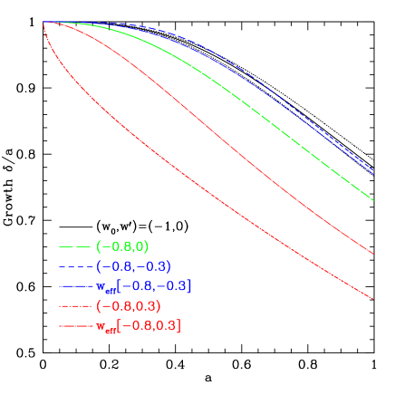
Figure 1: Growth factor of linear density perturbations plotted vs. scale factor $a=(1+z)^{-1}$ for six dark energy models with $\Omega_{m}=0.3$. Dotted curves show the effect of changing $\Omega_{m}$ by $\pm 0.02$ for the cosmological constant case. Curves labeled $w_{eff}$ use the constant equation of state that gives the same distance to the last scattering surface as the bracketed models, and hence are degenerate with respect to the CMB.

However, the class of models with $w^{\prime}>0$ exhibits dramatically different behavior. This includes what we chose as our fiducial model to test time varying EOS, the supergravity inspired model SUGRA of Brax & Martin (1999) that is well fit by $w_{0}=-0.82$, $w_{a}=0.58$ (i.e. $w^{\prime}=+0.29$). Note that Linder (2002a) has shown that the fit is good to 3% in $w$ at $z=1.7$ and to 0.2% in distance to the last scattering surface at $z=1089$.

Models with $w^{\prime}>0$ show definite differences in the growth of structure from a cosmological constant universe. For a model like SUGRA (here actually $w_{0}=-0.8$, $w^{\prime}=0.3$) the growth disparity reaches 26% at the present day. The figure shows two other points of interest. Comparing SUGRA to the constant EOS model that matches its distance to the last scattering surface, and so effectively mimics the time varying model as far as CMB data is concerned (except at low multipoles), the difference in total growth is 12%. That is, the time varying model and the constant, effective model can be distinguished through large scale structure information, despite being largely degenerate in their CMB power spectra. This is a promising sign.

The other interesting element is that even at high redshift the time varying model with $w^{\prime}>0$ possesses different behavior from the cosmological constant and other constant $w$ models. This shows the influence of dark energy at early times is very different from the cosmological constant, which quickly becomes dynamically negligible for $z>1$. Such a characteristic offers the possibility that evidence for time varying EOS dark energy might be found as well in the low multipole region of the CMB power spectrum (see Caldwell et al., 2003, for a discussion of the influence of “early quintessence” on the CMB through the integrated Sachs-Wolfe effect).

So three avenues appear to be open for the detection of physically important properties of dark energy from its influence on large scale structure: 1) linear growth rate, 2) nonlinear structure formation and evolution, and 3) large angle power in the CMB power spectrum. In the remainder of this section we investigate further the first avenue and then proceed in §4 to discuss numerical simulations of the second possibility (see Benabed & Bernadeau, 2001, for an analytic attempt). The third approach has been addressed by Hu (2002) with not very optimistic conclusions (but see Cooray, Huterer & Baumann, 2003).

Somewhat different results for the linear growth rate appear if we change the measurement technique. Suppose that rather than normalizing the density perturbations by their high redshift behavior (currently corresponding to COBE/WMAP normalisation of the matter power spectrum, though Planck will provide great improvement), we calibrate them by their present amplitude. This is like fixing $\sigma_{8}$, the power on the interface of linear/nonlinear scales. While observations have not yet determined this precisely, we can explore the consequences. As seen in Fig. 2, now the models are difficult to distinguish at low redshifts and there is near degeneracy in the growth factor between the time varying model and the effective constant $w$ model that matches it with respect to the CMB.

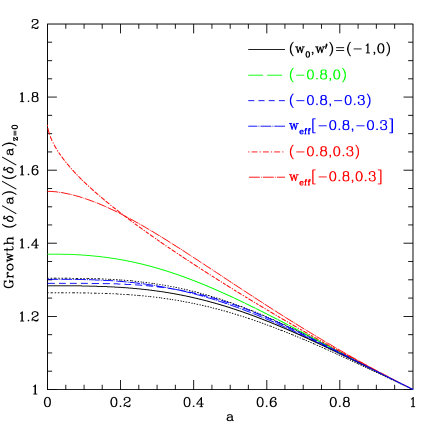
Figure 2: Same as Fig. 1 but with the growth factors normalized by their values today. The present growth, related to the mass variance $\sigma_{8}$, is not yet precisely known, however.

The issue of the optimal way to measure the growth factor through the matter power spectrum is an area of ongoing research, increasingly important with the future advanced large scale structure surveys. Perhaps the most realistic observable for now is the ratio of growth factors at different redshifts, a measure of the evolution of structure. This will carry correspondingly less content since it is only a relative measure, without information from the absolute level. Such a ratio could be read off from either Fig. 1 or 2 and indeed can be seen to vary little with cosmological model. For example, the evolution between $z=2$ and $z=1$ in the models with $(w_{0},w_{a})=(-0.8,0)$ or $(-0.8,0.3)$ agrees with the evolution in the cosmological constant model to 2% or 5%. This casts strong doubt on the idea that the growth evolution of large scale structure by itself (without a precise and robust high redshift, CMB normalisation) is useful as a probe of dark energy.

3.2 Sensitivity of Linear Growth Rate to Dark Energy

To understand the use of the evolution of linear matter density perturbations for probing the dark energy, we need to study not just the gross differences in the curves in Fig. 1 but the details of how they depend on dark energy properties and other cosmological parameters. We use the Fisher matrix formalism (see, e.g., Tegmark et al., 1998) to plot the sensitivity of the growth to the parameters $\Omega_{m}$, $w_{0}$, and $w_{a}$ in Fig. 3. The sensitivity increases toward low redshift since this corresponds to more time for the differing growth dynamics to take effect.

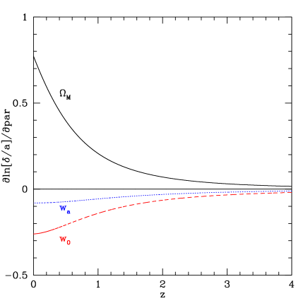
Figure 3: Logarithmic sensitivity of the growth factor to the cosmological parameters, perturbed around the cosmological constant model, as a function of redshift. Such a plot is useful in finding lower bounds to parameter estimation errors and in indicating degeneracies between parameters.

Besides the sensitivity, the degeneracy between parameters is a crucial aspect to the usefulness of the probe. The similarity of the shapes of the $w_{0}$ and $w_{a}$ curves guarantees a strong degeneracy between them, apart from further interaction with the value of $\Omega_{m}$. Combined with the relatively low accuracy achievable on the growth factor from observations, this leads to the growth factor by itself – even with the initial amplitude known – not serving as a precision cosmological probe. For example, even if all other parameters were fixed, a 5% determination of $\delta/a$ at $z=1$, say, would only constrain $w_{0}$ to $\pm 0.35$. And degeneracies strongly amplify the uncertainty. Additionally, the degeneracy direction in the $w_{0}-w_{a}$ plane is roughly aligned with the contours from the CMB, so the growth factor possesses little complementarity with the CMB and only a modest amount with the supernova distance measure.

For the simulated data sets we consider a measurement of the growth factor to 5% (equivalent to 10% determination of the linear power spectrum) at three values of the scale factor (equivalent to $z=0.67$, 1.5, 4), SNAP supernova measurements (including systematic uncertainties), and Planck CMB determination of the angular distance to the last scattering surface (normalisation of the primordial power is implicit in the growth factor measurement). The results, shown in Fig. 4, are not sensitive to the exact redshifts chosen for the growth factor estimates. Addition of growth information improves constraint of $w_{0}$, $w_{a}$ by less than 2%. This holds as well if the growth factor is normalized to $z=0$.

However, as was found for the baryon oscillation method (Linder, 2003b), the situation changes dramatically when the fiducial dark energy model is not taken to be the cosmological constant but the SUGRA model with time varying EOS. Now the growth factor under the influence of the dynamic field has a different cosmological dependence and possesses substantial complementarity with both the supernova and CMB data, as shown in Fig. 5. The parameter uncertainties using all three methods in synergy become $\sigma(w_{0})=0.04$, $\sigma(w^{\prime})=0.05$ (recall that $w^{\prime}=w_{a}/2$). That gives a 6$\sigma$ detection of time variation in the EOS!

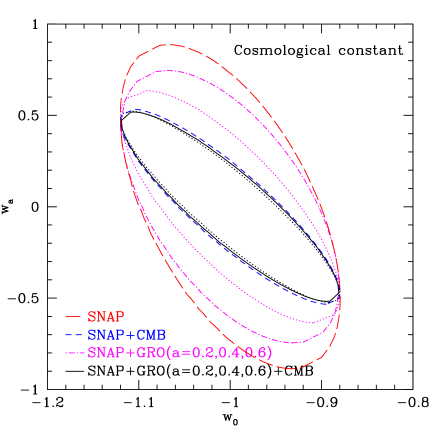
Figure 4: Parameter estimations (68% confidence level) of the present equation of state and its time variation, marginalizing over the matter density $\Omega_{m}$ with a prior of $\sigma(\Omega_{m})=0.03$. Dotted curves use the growth factor normalized to its value today. The growth factor alone (not shown) is poor in constraining the cosmological model, and offers little complementary leverage for the proposed SNAP supernova survey, and none in addition to SNAP plus the Planck CMB survey.

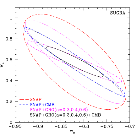
Figure 5: Same as Fig. 4 but for dark energy following the SUGRA model, with present equation of state $w_{0}=-0.82$ and time variation $w_{a}=0.58$. In this case, information on the linear growth factor adds valuable constraints.

A further interesting characteristic of the growth factor is a sufficiently distinct cosmological dynamics dependence to break some degeneracies outside the dark energy framework. For example, the braneworld model with crossover scale $H_{0}r_{c}=1.43$ discussed in Linder (2003a), difficult to distinguish from a $w=-0.7$ dark energy model through the distance relation ($<0.5\%$ difference), does differ by $\sim 4\%$ in the growth factor (though not when normalized at low redshift). This illustrates the utility of the $\delta H^{2}$ formalism of §2 for testing the cosmological framework.

3.3 Growth Rate and Weak Gravitational Lensing

One of the main applications of the growth rate is to cosmological observables that statistically characterize large scale structure. In §4 we address how the ingredient of the linear growth factor enters description of nonlinear structure. But here we make a brief, illustrative foray into the linear regime of the weak lensing shear used to map out the matter distribution (including dark matter) through its gravitational deflection of light from distant sources.

Observations of such shear are becoming increasingly useful cosmological tools and depend on the primordial matter density power spectrum, the growth rate, and geometric distance factors. We examine the simplified, though central, quantity of the shear linear lensing power spectrum (cf. Jain & Seljak, 1997; Huterer, 2002):

$$C_{\ell}\sim\int_{0}^{z_{s}}dz_{l}\,\left[\Omega_{m}(1+z_{l})\left(r_{ls}\over r_{s}\right)\,G(z_{l})\right]^{2}{1\over H(z_{l})\,r_{l}}\,.$$ (12)

Here $z_{l}$ is the redshift of the lensing mass, $z_{s}$ of the source galaxy, $r_{s}$ the comoving distance to the source, and $r_{ls}$ the comoving distance between the source and the lens. For simplicity we used the linear matter power spectrum $P_{k}\sim k\,G^{2}$ and fix $z_{s}$. The latter corresponds to having tomographic information.

We find that this lensing combination alone cannot place useful constraints on the dark energy but it does have good complementarity with the supernova distance measurements. Such lensing data strongly improves the determination of $\Omega_{m}$, as traditionally expected, and reduces uncertainty in the time variation $w_{a}$ slightly more dramatically than CMB information. However it has little complementarity with CMB data, and so the limits are not much further improved (1%) on inclusion of both lensing and CMB data. Fig. 6 shows the case of 5% determination of the weak lensing shear power spectrum at $z_{s}=1.5$. Results are not very sensitive to the exact redshift, or combination, chosen. The SUGRA case leads to similar conclusions, though there the weak lensing has more complementarity with the CMB and adding the lensing information tightens the constraints on $w_{0}$ and $w_{a}$ from supernovae and CMB by 34%. Thus the SNAP weak lensing program in combination with the SNAP supernova survey provides an important crosscheck on the results from SNAP supernovae plus CMB, plus the possibility of additional improvements.

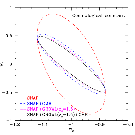
Figure 6: Parameter estimations (68% confidence level) of dark energy properties using future 5% measurement of the weak gravitational lensing linear power spectrum in addition to SNAP supernova distances and Planck CMB data. The lensing power has good complementarity with supernovae, though little with the CMB. Thus supernovae plus lensing should provide a valuable crosscheck on supernovae plus CMB results.

Of course the probe may be further strengthened by using information from the nonlinear part of the power spectrum. To employ the nonlinear regime, one needs to carry out numerical simulations including a time varying EOS or use fitting formulas valid for such cases, neither of which previously existed. In the remainder of the paper we present and discuss such a simulation.

4 A Simulation of Large Scale Structure Formation

So far in this paper we have concentrated on the dependence of the linear growth factor on the nature of the dark energy. In this section we turn our attention to the influence of the dark energy on the growth of non-linear large-scale structure – specifically the dark matter halo mass function. This measure of the number density of objects as a function of mass is important in a wide range of large-scale structure areas, including the use as a probe of the cosmological model.

Theoretically the dark matter halo mass function has been explored in CDM models mainly through n-body simulations e.g. Efstathiou et al. (1988); Lacey & Cole (1994); Gross et al. (1998); Governato et al. (1999); Jenkins et al. (2001); White (2001, 2002). Nearly all simulations to date focussing on this issue have modelled a universe in which the dark energy is static – a cosmolological constant $\Lambda$ – and the matter component is exclusively dark – and have ignored the fluid and dissipative nature of the baryonic component. The baryons are taken into account when computing the input matter transfer function used in making the initial conditions for the simulation. In the simulation itself it is assumed that the baryons behave as a pressureless component which mirrors the dark matter precisely. Modelling of the formation of individual haloes where a baryonic component is included, for example the Santa Barbara cluster comparison project (Frenk et al., 1999), lends support to the idea that one can determine the mass function for virialised dark matter haloes well without including the baryons at least for the high mass end.

At the same time as progress has been made studying the mass function using n-body simulations, analytic formulae have been developed to describe the mass functions. The most influential work was pioneered by Press & Schechter (1974) which utilises the spherical top-hat model of collapse. Comparisons of the Press-Schechter mass function to n-body simulations by a number of authors have noted that the Press-Schechter mass function tends to overestimate the mass function at low masses and underestimate the high mass end. This discrepancy has led to the development of improved analytic mass function formulae, such as the work of Sheth & Tormen (1999); Sheth, Mo & Tormen (2001); Sheth & Tormen (2002) (S-T hereafter), based on a model which accounts for ellipsoidal rather than spherical collapse. However in this paper we will concentrate on the ‘universal’ mass function formula presented in Jenkins et al. (2001) (J01 hereafter), which is an empirical fit to a wide range of simulation data (of which those used by S-T form a subset). As we will show in the next section this formula does actually predict the mass functions in a SUGRA quintessence model without needing modification.

Both simulations and the analytic formulae show for CDM models with Gaussian power spectra that the high mass end of the halo mass function is very sensitive to the precise normalisation of the power spectrum. If one can by some means determine the halo mass function over a range of redshifts then in principle one can find how the linear growth factor evolves as a function of redshift for the universe.

The dark matter halo mass function is not directly observable, though future observations exploiting weak gravitational lensing will make progress in this direction. However it is believed that the largest dark matter haloes are recognisable because they host galaxy clusters. Galaxy clusters contain, as well as galaxies, copious amounts of x-ray emitting gas. The presence of x-ray emitting gas not only signals the presence of the cluster halo which helps to find and count them, but can also be exploited to estimate the actual mass of the surrounding dark matter halo in a variety of ways. Estimates of the halo mass function using observational data of galaxy clusters have been made and utilised by many authors to estimate the value of the matter power quantity $\sigma_{8}$ locally - e.g. White, Efstathiou & Frenk (1993),Viana & Liddle (1996), Eke, Cole & Frenk (1996), Seljak (2002). Observations of clusters over a range of redshifts potentially enables the evolution of the growth factor to be determined. Two difficulties to surmount in using clusters as cosmological probes are the relation of the observables to theoretical characteristics, e.g. mass, and then the extraction of cosmological parameters free from astrophysical factors and degeneracies. The typical uncertainty in the theoretically determined mass functions are around 10%. However making accurate mass estimates of galaxy clusters is far from easy and comparing an observationally determined mass function with the relatively clean theoretical mass function requires extensive and detailed modelling - it is not our aim in this paper to discuss these important aspects.

As mentioned above the mass function formula given in J01 is a fit to the mass functions from a range of CDM simulations. These simulations include models with a cosmological constant ($w=-1$) and Open models which have an effective value of $w=-1/3$. The values of interest for $w$ for the dark energy are typically within the range that has already been studied so it would not seem too surprising if the mass function for models with constant values of $w$ intermediate between $-1/3$ and $-1$ are accurately predicted by existing mass function formulae. However it is interesting to ask how the mass function of a model where the value of $w$ is rapidly changing compares to the predictions. The SUGRA model of Brax & Martin (1999) is an attractive model to choose for this reason because the value of $w$ evolves reasonably rapidly.

The part of the mass function which is most sensitive to the linear growth factor is the high mass end where the mass function falls off steeply. One would similarly expect that it would be this region of the mass function that would show the greatest sensitivity to a time variation in $w$. We therefore have designed our simulation to model a large volume of space so that we can measure the abundance of very massive, but rare, clusters.

As far as we are aware the only simulations with a quintessence component with a changing EOS are those of Klypin et al. (2003) who also model the SUGRA quintessence together with a model by Ratra & Peebles (1988), which has a much more gently changing value of $w$, and some models with constant $w$. Their simulations have very good spatial and mass resolution, allowing them to study the properties of individual dark matter haloes in some detail. However their simulation cubes are relatively small compared to ours: even their largest simulation cube is some 66 times smaller in volume than our cube. The results the authors report for the mass functions determined from their simulations appear to be fully consistent with our own results. Our simulations are designed to give better statistics at the high mass end of the mass function and are in this sense complementary.

Below we describe the n-body code, the parameter choices for the simulation and the initial conditions for the simulation. The results themselves are reported in the section 5.

4.1 Code details.

We have used the publicly available parallel code GADGET (v1.1) described in Springel, Yoshida & White (2001) to perform the n-body simulation. We modified the code to allow the inclusion of a quintessence component with an EOS of the form $w(a)=w_{0}+(1-a)w_{a}$, where $a$ is the expansion factor defined so that $a=1$ at the present epoch. The only modifications required to the code were to update expressions for the Hubble parameter to include the quintessence component. We verified these modifications by checking that the modified code can reproduce the correct linear growth rates on a series of test simulations. We will only report the results of this test for the simulation presented here.

We determined the linear growth rates from the n-body simulation by measuring the power associated with the longest wavelength modes of the simulation box for the initial conditions and for each output. The longest wavelength modes are least affected by non-linear effects. For comparison we also computed the growth rates by numerical integration of equation (11). Between z=38.9 and z=2 the agreement in the growth factors measured from the simulation and computed by numerical quadrature is better than 0.2%. This is a non-trivial test that the code can handle a quintessence component because the SUGRA model has an EOS $w=-0.25$ at the upper redshift and by redshift 2 the quintessence component already has a significant dynamical influence: for example the value of $G(a)$ is 0.84 rather than unity as it would be in a matter dominated universe. The long wavelength modes grow slightly more slowly than the linear theory prediction, due we believe to non-linear effects (see Baugh & Efstathiou, 1999). By z=0, when the long wavelength density fluctuations themselves have an amplitude of a few percent, the agreement is better than 0.8%. By comparison this difference is 25 times smaller than the difference of the growth rates of the quintessence model and $\Lambda$CDM over the same interval.

4.2 Simulation details.

We have designed the simulation with two aims in mind:       (i) to determine the high end of the halo mass function, and (ii) to match as closely as possible, at redshift zero, the parameters of an existing $\Lambda$CDM simulation so that a direct comparison can be made. The most suitable reference $\Lambda$CDM simulation for determining the high mass end of the halo mass function is the $\Lambda$CDM Hubble volume run described in Evrard et al. (2002) which models a cube, $3000h^{-1}{\rm Mpc}$ on a side. We have therefore selected the same values for the matter density, $\Omega_{m}$, the particle mass and the gravitational softening length as the $\Lambda$CDM Hubble simulation. We also match very closely the power spectrum shape and amplitude of the linearly extrapolated power spectrum at redshift zero to those of the $\Lambda$CDM Hubble simulation. Our simulation volume is significantly smaller than the $\Lambda$CDM Hubble simulation at $648h^{-1}{\rm Mpc}$ on a side.

We have chosen a quintessence component with a variable value of $w$. As discussed earlier, the choice $w_{0}=-0.82$, $w_{a}=0.58$, gives a good fit to the SUGRA quintessence model. We will refer to our simulation as the SUGRA-QCDM model. The parameters of the simulation are listed in table 1.

The initial conditions were generated by the serial version of the code that was used to generate the initial conditions for the Hubble volume simulations (Evrard et al., 2002). The initial conditions are created from an initially uniform particle distribution (in this case a glass distribution generated in the way described by White, 1996) by perturbing the particles to give the desired power spectrum and using the Zel’dovich approximation (Zel’dovich, 1970) to assign velocities to each particle which are proportional to the displacements. The code needed to be altered to give the correct constant of proportionality, which depends on the logarithmic growth ${\rm d}\ln D/{\rm d}\ln a$, when assigning the velocities. The difference in this constant between an Einstein-deSitter ($\Omega_{m}=1$) and quintessence model at the start redshift is small - only $\sim 1.5\%$ - though this is much larger than the difference between a matter dominated and cosmological constant model.

Table 1: Parameters of the SUGRA-QCDM n-body simulation - the mass resolution, softening and power spectrum normalisation are chosen to match the $\Lambda$CDM Hubble volume simulation described in Evrard et al 2002. $\sigma_{8}$ is the RMS of the linear density field smoothed with a top-hat filter of $8h^{-1}{\rm Mpc}$ in radius.

Parameter		Value
$\Omega_{m}$		0.30
$w_{0}$		-0.82
$w_{a}$		0.58
$\sigma_{8}(z=0)$		0.90
Box size/$h^{-1}{\rm Mpc}$		648
Number of particles		10077696
Particle mass/$10^{12}h^{-1}M_{\odot}$		2.25
Comoving softening length/$h^{-1}{\rm Mpc}$		0.1

5 Simulation Results

The simulation was started at z=38.9 and outputs were made at redshifts z = 3, 2, 1.5, 1, 0.5, 0.25 and 0.

5.1 The mass function at z=0

To begin with we will compare the mass functions at redshift zero. The z=0 linear power spectrum of the SUGRA-QCDM simulation has the same shape and amplitude as the $\Lambda$CDM Hubble simulation by design. Analytical fitting formulae for mass functions such as Press & Schechter (1974), S-T and Jenkins et al. (2001), all predict that the CDM mass function depends primarily on the linear power spectrum. We would therefore expect if one extrapolates these results to quintessence models that our two models should have very similar mass functions at redshift zero.

One potential complication in comparing two different cosmological models lies in the problem of how to define the haloes in a consistent way so that they can be compared. A common approach to this problem is to use the spherical top-hat collapse model to give guidance as to the expected collapse overdensity of virialised objects - e.g. Lacey & Cole (1993); Eke, Cole & Frenk (1996). Following these arguments would lead to different values for the overdensity for haloes selected in $\Lambda$CDM and SUGRA-QCDM.

However we can circumvent these issues by adopting the halo definition used in J01. The haloes are defined using the friends-of-friends algorithm (Davis et al., 1985) with a linking length of b=0.2. J01 showed that using this way of defining haloes it is possible to fit the mass functions for CDM models with a wide range of cosmological parameters and redshifts with a single ‘universal’ fitting formula which is accurate to better than 20%. It is this simplicity which motivates our choice of halo definition. In this subsection we will compare the SUGRA-QCDM and $\Lambda$CDM simulations at z=0 directly.

Our ability to determine the mass function is limited by a number of considerations. At the high mass end, where the objects themselves are resolved with the largest numbers of particles, the main limitation in determining the mass function is the volume of the box. We plot the mass functions only up to the point where the Poisson error reaches 10%. At the low mass end the situation is less simple. One would expect determination of the mass function to be less and less reliable as one resolves haloes with fewer and fewer particles. We take a limit of 20 particles as the minimum number of particles. This limit is supported by tests presented in appendix A of J01 where they compare the mass functions from simulations with the same mass resolution as our SUGRA-QCDM simulation to those from simulations with superior mass resolution.

In figure 7 we show the SUGRA-QCDM and $\Lambda$CDM mass function evaluated with the FOF(b=0.2) group finder. The mass functions from both simulations have been smoothed using an identical Gaussian with an RMS width of 0.08 dex. The mass functions agree very well - the differences are below 10%. This is an encouraging result ( a similar result is also seen in Klypin et al., 2003) and suggests that it should be possible to predict the mass functions for this and other quintessence models with a smoothly varying value of $w$ with a precision of $\sim 10$% from a knowledge of just the linearly evolved power spectrum. In the next section we will compare the SUGRA-QCDM mass function with the universal mass function formula of J01 directly for several redshifts.

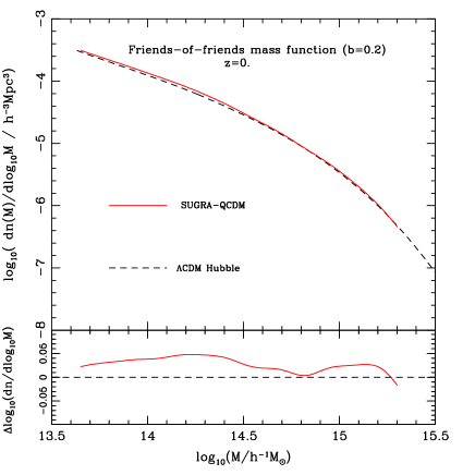
Figure 7: Top panel: the dark matter halo mass function defined using the friends-of-friends algorithm with a linking length of 0.2. The mass functions of $\Lambda$CDM Hubble simulations and SUGRA-QCDM that at z=0 have nearly identical power spectra are very similar. The mass functions are plotted for haloes of 20 particles and more and up to an upper mass cut-off where the Poisson uncertainty in the mass function first exceeds 10%. Bottom panel: the solid curve shows the difference between the SUGRA-QCDM mass function and the $\Lambda$CDM Hubble volume mass function. The differences are below 10%.

5.2 The mass function at all redshifts

Here we will plot the combined mass functions at redshifts 3, 2, 1.5, 1, 0.5, 0.25 and 0 for the SUGRA-QCDM run and compare them with the J01 mass function formula. But we first repeat a few definitions, adapted from J01, which are required further on.

It is convenient to use as an effective mass variable, $\ln\sigma^{-1}$, where $\sigma(M)$ is the RMS of the linear density field smoothed with a top-hat filter containing mass $M$ at the mean density. This is defined as:

$$\sigma^{2}(M,z)={D^{2}(z)\over 2\pi^{2}}\int_{0}^{\infty}k^{2}P(k)W^{2}(k;M){\rm d}k,$$ (13)

where $D(z)$ is the growth factor of linear perturbations normalised so that $D(0)=1$, $P(k)$ is the linear power spectrum at redshift zero and $W(k;M)$ is the Fourier-space representation of a real-space top-hat filter enclosing mass $M$ at the mean density of the universe.

We define the mass function $f(\ln\sigma^{-1},z)$ through:

$$f(\ln\sigma^{-1},z)\equiv\frac{M}{\rho_{0}}{{\rm d}n(M,z)\over{\rm d}\ln\sigma^{-1}},$$ (14)

where $n(M,z)$ is the abundance of halos with mass less than $M$ at redshift $z$, and $\rho_{0}(z)$ is the mean density of the universe at that time. With these definitions we can plot the mass functions for any CDM model and at any redshift conveniently onto the $\ln f-\ln\sigma^{-1}$ plane.

Figure 8 shows the mass functions for the SUGRA-QCDM simulation, plotted in the $\ln f-\ln\sigma^{-1}$ plane, for redshifts $z$= 0, 0.25, 0.5, 1.0, 1.5, 2 and 3. The mass functions are plotted as dashed lines for haloes of 20 particles and more (as in J01) and cut-off at the high mass end when the Poisson errors reach 10%. The simulation curves have been smoothed using a Gaussian with an RMS of 0.05 dex. The solid line shows the J01 universal mass function fit given by:

$$\phantom{xxxxxxx}f(\ln\sigma^{-1})=0.315\;\exp\big{[}-|\ln\sigma^{-1}+0.61|^{3.8}\big{]},$$ (15)

valid over the range $-1.2\leq\ln\sigma^{-1}\leq 1.05$, and the flanking dotted lines denote a 20% uncertainty about this fit. These curves are similarly convolved with a 0.05 dex Gaussian.

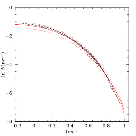
Figure 8: The halo mass functions for the SUGRA-QCDM simulation plotted in the $f-\ln\sigma^{-1}$ plane for redshifts 0,0.25,0.5,1,2,3. The smooth solid curve flanked by dotted curves marks the J01 universal mass function formula. The dotted lines mark a $\pm 20$% uncertainty in the mass predicted mass function. The SUGRA-QCDM mass functions are plotted for groups of 20 or more particles and up to the point where the Poisson error becomes 10%. The SUGRA-QCDM mass function is well fit by the Jenkins et al formula. Some departure is apparent at high values of $\ln\sigma^{-1}>0.85$, but as discussed in the text the origin of this departure is likely due to numerical limitations rather than being real.

Note that the universal nature does not imply that different models predict the same observable consequences, only that they can be treated by the same parametrization. Each model is distinguished by its particular $\sigma^{2}(M,z)$ relation.

The main result of this section is that the SUGRA-QCDM mass function is well fit by the J01 formula - at least to the same degree of accuracy as was found for a host of other CDM cosmological models. The fit is good despite the fact that this model has a changing value of $w$. It therefore seems likely that the J01 should work well for a wide range of dark energy models. Although we have used the J01 formula in figure 8 we could instead have used the formula of S-T. Klypin et al. (2003) find that the S-T formula provides an excellent fit to their mass functions. We do find however that for $\ln\sigma^{-1}$ above about 0.75 that J01 formula is definitely a better fit, with the S-T formula tending to overpredict the number of haloes.

It is apparent from figure 8 that the most significant deviation away from J01 formula occurs for $\ln\sigma^{-1}>0.85$, where only the $z=3$ output contributes. A closer analysis of this curve and other curves shows that the plotted mass functions tend to drop away relative to the J01 curve for small numbers of particles per group. This drop off is particularly apparent for the $z=$ 3 and 2 outputs where the mass function is steep. The cause of this feature is unclear but is likely numerical in origin. The influence of the dark energy component diminishes as one goes to higher redshift and the J01 formula works well for matter dominated models - so if anything one would expect the degree of fit to improve with increasing redshift contrary to what is seen. This divergence is much less pronounced at lower redshift and is not apparent in the resolution tests presented in appendix A of J01 for the Hubble volume simulations which are for redshift zero.

To conclude, firstly we have found in this section that the $z=0$ mass functions of the Hubble $\Lambda$CDM simulation and our own SUGRA-QCDM simulation match to a precision of better than 10% in abundance for haloes in the mass range of $4.5\times 10^{13}-2\times 10^{15}h^{-1}M_{\odot}$. By design, the $z=0$ linear power spectrum of the two models was closely matched. The results indicate that the mass function depends primarily on the linear power spectrum and is only very weakly if at all dependent on the details of the expansion history. Secondly, from an analysis of the SUGRA-QCDM mass function at a range of redshifts we find that mass function formulae such as J01 and S-T provide good estimates of the halo mass function for flat quintessence models. The J01 formula gives a better fit at the high mass end than S-T for $\ln\sigma^{-1}>0.75$. The goodness of fit is comparable with that found when comparing these formulae to the mass functions determined from the following cosmological models: matter dominated, open, and flat models with a cosmological constant. We are able to verify the accuracy of the fit over range $-0.2<\ln\sigma^{-1}<0.85$ from our simulation.

These results imply that the main observational discriminators for large-scale structure between cosmological models are: the present linear power spectrum, to be fixed by wide field surveys; the linear growth factor, discussed in the first part of this paper and probed by future deep surveys; and distances and volumes measured by expansion history mappers such as SNAP.

6 Conclusions

Cosmic structure formation and evolution provides an additional path to exploring the cosmological model besides mapping the expansion history. Many of the observational probes employing structure rely on the growth dynamics of density fluctuations, in either the linear or nonlinear regime.

Linear perturbations offer the best hope of structure measurements with relatively uncomplicated physics and clean observations free of many astrophysical entanglements. Analyzing the linear growth behavior, we find little leverage on the nature of the dark energy – unless it possesses a time varying equation of state. In this latter case the growth shows good complementarity with supernova and CMB measurements.

We have emphasized that such time variation appears generically in proposed dark energy models other than the cosmological constant and can also be used to treat modifications of the cosmological framework.

The growth also enters as a contribution to the gravitational lensing power spectrum, and weak lensing as a cosmological probe promises interesting complementarity and crosschecks. Such a method can take advantage of both the linear and nonlinear density scales to attempt to balance sensitivity with systematic uncertainties.

For the nonlinear realm of structure, investigations at the level of precision necessary require numerical simulations. We present one of the first, and currently the largest volume, N-body simulation with a time varying equation of state. As a first application of the data, we calculate the halo counts as a function of mass, a quantity relevant to forthcoming structure surveys. We find that this is well fit by the previous Jenkins mass formula, extending its universality to time varying equations of state, at least at the 20% level. At redshift zero the dynamical dark energy model shows agreement to better than 10% with the cosmological constant simulation that matches the linear power spectrum today, suggesting this serves generally as a central quantity in describing structure formation.

Much work remains for the future to bring observations of structure to the level of theoretical and systematic uncertainty necessary for precision probing of dark energy. But the results here lay a foundation to build upon for using not only the expansion history of the universe but the growth history of structure in a rigorous quest to understand the physics behind the accelerating universe.

Appendix. Approximation of the Linear Growth Factor

Within the formalism of the Birkhoff’s theorem argument presented by Peebles (1980, 1993) for the evolution of linear density perturbations, one can write a closed form expression for the growth. However this does not hold for general cosmological models. While it was sufficient and indeed prescient for the main models considered in 1980, it neglects a term arising for a general pressure component (as Peebles alludes to); this term is proportional to $(1+3w)(1+w)\Omega_{w}$ and so we see that serendipitously the closed form is exact for a pure matter model (SCDM, $\Omega_{w}=0$), an open model (OCDM, $w=-1/3$), and a cosmological constant model ($\Lambda$CDM, $w=-1$). But a second order differential equation does not generally possess such a quadrature and instead an equation like Eq. (8) must be solved.

Fig. 9 shows the difference between the exact solution for the growth factor and the approximation given by the closed form

$$G_{approx}={5\over 2}\Omega_{m}{H\over a}\int_{0}^{a}da\,(aH)^{-3}\,.$$ (16)

The differences for the time varying SUGRA model can be $\sim 15\%$; this propagates into the power spectrum as the square, and then further as a possibly substantial bias on the cosmological parameters. The situation is better if future detailed observations allow use of the growth factor normalized to the present ($\sim 1\%$ difference for SUGRA, though $\sim 5\%$ for $w=-1.2$). See Wang & Steinhardt (1998) for a fitting function involving an integral over the equation of state, valid at high redshifts, for slow variations.

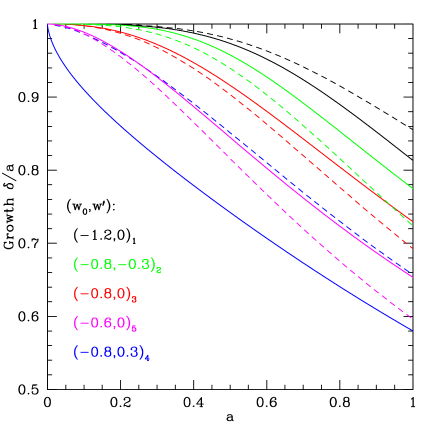
Figure 9: Comparison of the exact growth factor (solid curves) with the closed form approximation, Eq. 16 (dashed curves). The solid curves are labeled according to the vertical ordering, and the subscripts indicate the ordering of the dashed curves for those models. The approximation is insufficient for precision cosmology.

References

- Alam et al. (2003) Alam, U., Sahni, V., Saini, T.D., & Starobinsky, A., 2003, astro-ph/0303009
- Aldering et al. (2002) Aldering, G. et al., 2002, SPIE Proceeding 4835, astro-ph/0209550; http://snap.lbl.gov
- Baugh & Efstathiou (1999) Baugh, C. M. & Efstathiou, G. , 1994, MNRAS, 270, 183.
- Benabed & Bernadeau (2001) Benabed, K. & Bernadeau, F., 2001, Phys. Rev. D64, 083501
- Bond et al. (2002) Bond, J.R. et al., in Theoretical Physics, MRST2002, eds. V. Elias, R. Epp, R. Myers, astro-ph/0210007
- Brax & Martin (1999) Brax, P. & Martin, J., 1999, Phys. Lett. B, 468, 40
- Caldwell et al. (2003) Caldwell, R.R., et al., 2003, astro-ph/0302505
- Cooray, Huterer & Baumann (2003) Cooray, A., Huterer, D., & Baumann, D., 2003, astro-ph/0304268
- Davé, Caldwell, & Steinhardt (2003) Davé, R., Caldwell, R.R., & Steinhardt, P.J., 2002, Phys. Rev. D, 66, 023516
- Davis et al. (1985) Davis, M., Efstathiou, G., Frenk, C. S. & White, S. D. M., 1985, Ap.J, 292, 371.
- Efstathiou et al. (1988) Efstathiou, G., Frenk, C. S. & White, S. D. M., Davis, M., 1988, MNRAS, 235, 715
- Eke, Cole & Frenk (1996) Eke, V. R., Cole, S. & Frenk, C. S., 1996, MNRAS, 282, 263
- Evrard et al. (2002) Evrard, A. E., MacFarland, T. J., Couchman, H. M. P., Colberg, J. M., Yoshida, N., White, S. D. M., Jenkins, A., Frenk, C. S., Pearce, F. R., Peacock, J. A. & Thomas, P. A., 2002, ApJ, 573, 7.
- Frenk et al. (1999) Frenk et al , 1999, Ap.J, 525, 554.
- Governato et al. (1999) Governato, F., Babul, A., Quinn, T., Tozzi, P., Baugh, C. M., Katz, N. & Lake, G., 1999, MNRAS, 307, 949.
- Gross et al. (1998) Gross, M. K., Somerville, R. S., Primack, J. R., Holtzman, J. & Klypin, A., 1998, MNRAS, 301, 81.
- Hu (2002) Hu, W., 2002, Phys. Rev. D65, 023003
- Hu (2003) Hu, W., 2003, Phys. Rev. D66, 083515
- Huterer & Turner (2001) Huterer, D. & Turner, M.S., 2001, Phys. Rev. D64, 123527
- Huterer (2002) Huterer, D., 2002, Phys. Rev. D65, 063001
- Jain & Seljak (1997) Jain, B. & Seljak, U., 1997, ApJ, 484, 560
- Jenkins et al. (2001) Jenkins, A., Frenk, C. S., White, S. D. M., Colberg, J. M., Cole, S., Evrard, A. E., Couchman, H. M. P. & Yoshida, N., 2001, MNRAS, 321, 372.
- Klypin et al. (2003) Klypin, A., Maccio, A. V., Mainini, R. & Bonometto, S. A., 2003, astro-ph/0303304
- Knop et al. (2003) Knop, R. et al., 2003, ApJ in press.
- Lacey & Cole (1993) Lacey, C. G. & Cole, S., 1993, MNRAS, 262, 627.
- Lacey & Cole (1994) Lacey, C. G. & Cole, S., 1994, MNRAS, 271, 676.
- Linder (1988) Linder, E.V., 1988, Max-Planck-Institut (MPA) Research Note; Linder, E.V., 1997, First Principles of Cosmology (Addison-Wesley)
- Linder (2002a) Linder, E.V., 2002, in Proc. IDM2002, astro-ph/0210217
- Linder (2002b) Linder, E.V., 2002, astro-ph/0212301
- Linder (2003a) Linder, E.V., 2003, Phys. Rev. Lett., 90, 091301, astro-ph/0208512
- Linder (2003b) Linder, E.V., 2003, astro-ph/0304001
- Ma et al. (1999) Ma, C-P., Caldwell, R.R., Bode, P., & Wang, L., 1999, ApJ, 521, L1
- Peebles (1980) Peebles, P.J.E., 1980, Large-Scale Structure of the Universe (Princeton U. Press)
- Peebles (1993) Peebles, P.J.E., 1993, Principles of Physical Cosmology (Princeton U. Press)
- Percival et al. (2002) Percival, W.J. et al., 2002, MNRAS, 337, 1068
- Perlmutter et al. (1999) Perlmutter, S. et al., 1999, ApJ, 517, 565
- Press & Schechter (1974) Press, W. H. & Schechter, P., 1974, Ap.J, 187, 125.
- Ratra & Peebles (1988) Ratra, B. & Peebles, P. J. E., 1988, Phys.Rev.D, 37, 3406.
- Riess et al. (1998) Riess, A.G. et al., 1998, AJ, 116, 1009
- Seljak (2002) Seljak, U., 2002, MNRAS, 337, 769
- Sheth & Tormen (1999) Sheth, R. & Tormen, G., 1999, MNRAS, 308, 119.
- Sheth, Mo & Tormen (2001) Sheth, R., Mo, H. J. & Tormen, G., 2001, MNRAS, 308, 119.
- Sheth & Tormen (2002) Sheth, R. & Tormen, G., 2002, MNRAS, 329, 61.
- Spergel et al. (2003) Spergel, D.N. et al., 2003, astro-ph/0302209
- Springel, Yoshida & White (2001) Springel, V., Yoshida, N. & White, S. D. M., 2001, New Ast, 6, 79.
- Tegmark et al. (1998) Tegmark, M., Eisenstein, D.J., Hu, W., & Kron, R., 1998, astro-ph/9805117
- Viana & Liddle (1996) Viana, P. T. P. & Liddle, A. R., 1996, MNRAS, 281, 323
- Wang & Steinhardt (1998) Wang, L. & Steinhardt, P.J., 1998, ApJ, 508, 483
- White (2001) White, M., 2002, A&A, 367, 27.
- White (2002) White, M., 2002, Ap.J.sup, 143, 241.
- White (1996) White, S. D. M., 1996, Cosmology & Large-scale structure, Elsevier, Dordrecht, eds Shaefer, R., Silk, J., Spiro, M., & Zinn-Justin, J.
- White, Efstathiou & Frenk (1993) White, S. D. M., Efstathiou, G. & Frenk, C. S., 1993, MNRAS, 262, 1023.
- Zel’dovich (1970) Zel’dovich, Ya. B, 1970, A&A 5, 84.