Intracluster stellar population properties from N-body cosmological simulations – I. Constraints at $z=0$

Abstract

We use a high resolution collisionless simulation of a Virgo–like cluster in a $\Lambda$CDM cosmology to determine the velocity and clustering properties of the diffuse stellar component in the intracluster region at the present epoch. The simulated cluster builds up hierarchically and tidal interactions between member galaxies and the cluster potential produce a diffuse stellar component free-flying in the intracluster medium. Here we adopt an empirical scheme to identify tracers of the stellar component in the simulation and hence study its properties. We find that at $z=0$ the intracluster stellar light is mostly unrelaxed in velocity space and clustered in structures whose typical clustering radii are about 50 kpc at R=400–500 kpc from the cluster center, and predict the radial velocity distribution expected in spectroscopic follow-up surveys. Finally, we compare the spatial clustering in the simulation with the properties of the Virgo intracluster stellar population, as traced by ongoing intracluster planetary nebulae surveys in Virgo. The preliminary results indicate a substantial agreement with the observed clustering properties of the diffuse stellar population in Virgo.

1 Introduction

The diffuse light in nearby galaxy clusters is now clearly detected (Feldmeier et al., 2002) and its properties can be mapped via the Intracluster Planetary Nebulae (ICPNe hereafter) out to large radii (Arnaboldi et al., 1996; Theuns & Warren, 1997; Ciardullo et al., 1998; Feldmeier et al., 1998; Arnaboldi et al., 2002; Okamura et al., 2002; Arnaboldi et al., 2003). Recently, a complete sample of ICPNe identified by the [OIII] $\lambda$ 5007Å emission line in different fields in Virgo has been used in Aguerri et al. (2003, in preparation) to study the 2D spatial distribution of the diffuse intracluster stellar population.

While the presence of an intracluster stellar population (ICSP) has now been clearly demonstrated, its origin, time of formation, spatial distribution, and even its mass compared to that of the total stellar population are still largely unknown. Different cluster formation mechanisms might predict, at the present epoch, different spatial distributions or distribution functions for the ICSP that can be tested against the 2-dimensional (2D) projected distribution of ICPNe and their radial velocities.

Merritt (1984) proposed a model where the morphology distribution of galaxies in clusters is fixed during the cluster collapse and changes very little afterward. In this picture, tidal interactions have very limited effects on galaxies, with only those galaxies that are located deep in the cluster potential being affected. In such a model, the ICSP is removed from galaxies early during the cluster collapse, and its distribution is predicted to follow closely that of galaxies.

In the currently favored hierarchical clustering scenario, fast encounters and tidal interactions within the cluster potential are the main players of the morphological evolution of galaxies in clusters. “Galaxy harassment” (Moore et al., 1996) and “tidal stirring” (Mayer et al., 2001) cause a significant fraction of the stellar component in individual galaxies to be stripped and dispersed within the cluster in a few dynamical times. If the time scale for significant phase–mixing is longer than a Hubble time (or of the order of few cluster internal dynamical times), then the ICSP fraction should still be located in long streams along the orbits of the parent galaxies (as perhaps observed in Coma and Hydra, Calcáneo-Roldán et al., 2000). Detections of substructure in phase space (see analog in the Milky Way, Helmi, 2001) would be a clear sign of harassment as the origin of the ICSP. Dynamical properties of the ICSP are an important key in the puzzle of cluster evolution.

Until now, N-Body simulations have been used to investigate various observables in clusters of galaxies such as the density profiles (Navarro et al., 1997; Moore et al., 1998), projected galaxy number density (Moore et al., 1999b), dynamical properties of galaxies (Governato et al., 2001) and X-ray properties of the intracluster medium (Borgani et al., 2001). Dubinski (1998) studied the properties of the cluster stellar population in a CDM cosmological simulation, focussing on the origin of brightest cluster galaxies (BCGs). Semi-analytical models were used to study the properties of the baryonic component, e.g. the galaxy luminosity functions, Tully-Fisher and Faber-Jackson relations, number counts, the distribution of morphology, color and size, clustering strengths, and velocity dispersion profiles (Kauffmann et al., 1994; Cole et al., 1994; Guiderdoni et al., 1998; Mo et al., 1998; Governato et al., 1998; van den Bosch, 2000; Diaferio et al., 2001; Springel et al., 2001). However, this powerful approach is not able to follow in detail the dynamical evolution of the stellar component, once stripped from the parent galaxies.

We use here a cosmological N-body simulation to study the properties of the intracluster stellar population in a Virgo–like cluster at $z=0$, in a $\Lambda$CDM cosmology. N-body simulations for the dark matter component allow a larger number of particles and a larger dynamical range than simulations including an explicit treatment of hydrodynamics and star formation processes. Because stars are expected to form as gas cools at the bottom of the potential wells of dark matter halos (White & Rees, 1978), the simulated particles in the very high density regions (i.e. the center of DM halos) are likely to be good tracers of the stellar component. We therefore select as tracers of the stellar population those particles within local densities higher than $\sim 10^{4}$ times the critical density at any given time before $z\geq 0.25$, which is considered the epoch when the star formation stopped in the cluster.

This approach has some interesting advantages, when compared with the lower resolution hydrodynamical simulations with an explicit treatment of star formation. Namely we are able to follow the dynamical evolution of much smaller galaxies, and the higher numerical resolution helps to decrease significantly the numerical noise and the two–body relaxation, which can rapidly erase structures in the phase space.

The aim of this paper is to study the total amount of intracluster stellar light, the clustering properties, and the velocity distribution of the intracluster population of stars in a Virgo–like cluster in $\Lambda$CDM cosmology. We can then make predictions for observables such as the two-point angular correlation function (2PCF, hereafter) and the spatial correlation function (both of these computed via the LS estimator, see Appendix A) and the line of sight (LOS, hereafter) velocity distribution as expected in a present-day cluster. The former will be compared with the data samples now becoming available from wide field imaging surveys; the latter will soon be constrained by spectroscopical surveys with wide-field spectrographs. Linking the observable clustering and velocity properties of the ICSP with results from N-body simulations can in principle also be used to put constraints on the cluster formation epoch.

The paper is organised as follows: in Section 2 we describe the N-body cosmological simulations and the schema adopted to identify the ICSP; in Section 3 we describe the comparison with the observed datasets and the analysis of the velocity and clustering properties of the ICSP population; in Section 4 the dynamical characterisation of the intracluster stellar population is discussed. Conclusions are given in Section 5.

2 N-body Cosmological simulation

We have analysed a high resolution simulation of the formation of a galaxy cluster in $\Lambda$CDM cosmology (Governato, Ghigna & Moore, 2001), with $h_{0}$=0.7, $\sigma_{8}$=1, $\Omega_{0}$=0.3, $\Lambda$=0.7. The simulation was done using the so-called “renormalization technique” (Katz & White, 1993), with a total of 1.5 million particles, in a volume of 100 Mpc on a side. The cluster builds up hierarchically and has a typical merging history within the adopted cosmology, with a few groups being accreted at relatively low $z$. Tidal interactions between member galaxies and the cluster potential produce a diffuse stellar component free flying in the intracluster medium. At the end of the simulation, the cluster total mass is $\sim 3\times 10^{14}M_{\odot}$, similar to the Virgo cluster total mass, and half a million particles are within the cluster virial radius; each particle has a mass of $0.506\times 10^{9}M_{\odot}$. The spatial resolution is 2.5 kpc, which allows us to resolve substructures down to sub L_∗ scales. Several thousands of time steps were used to follow the simulation up to the present time. More details of the simulation are given in Governato, Ghigna & Moore (2001) and Borgani et al. (2001).

2.1 Tracing the stellar component

Following White & Rees (1978), the very high density regions at the center of DM halos are likely to be good tracers of the stellar component in galaxies. A simple criterion to select such tracers in an N-body simulation is via a density threshold; this is easily implemented and the implications can be studied in detail. We therefore select as tracers of the stellar population those particles in the simulation within local overdensities higher than $\sim 10^{4}$ times the critical density at any given time before $z\geq 0.25$, which is considered the epoch when the star formation stopped in the cluster.

For a fixed density threshold, the size of such an overdensity region varies with redshift, and for a given cosmological model depends mostly on the virial mass and concentration (Navarro et al., 1997; Bullock et al., 2001), and possibly on the accretion history of the dark halos (Wechsler et al., 2002; Zhao et al., 2002) because of the structure growth. The evolution with redshift of the overdensity regions in the growing halos is also determined by the cosmological model (see Navarro et al., 1997; Bullock et al., 2001, for a discussion). We estimated that the typical size of an overdensity region with 12000 times the critical density has a linear dimension of about 15 kpc at $z=0$ and 12 kpc at $z=3$ for a $M_{vir}=5\times 10^{12}h^{-1}M_{\odot}$ (a typical virial mass of a brightest cluster galaxy – BCG hereafter) and it is 7 kpc at $z=0$ and 5 kpc at $z=3$ for a virial mass of $M_{vir}=1.25\times 10^{12}h^{-1}M_{\odot}$ (Bullock et al., 2001; Wechsler et al., 2002; Zhao et al., 2002). Those particles within these scales experience local overdensities which are larger than the adopted threshold.

How do these overdensity regions compare with the optical radius of galaxies at different redshifts? Studies on the evolution of the linear scales of the luminous parts of galaxies suggest that they are a decreasing function of redshift; Nelson et al. (2002) found that the effective radius, $r_{e}$, for their galaxy sample decreases by a factor two at $z\sim 0.8$ with respect to the local values. Simard et al. (1999) showed that the total galaxy light is more concentrated at $z\sim 1$ with respect to local values.

This evidence implies that our simple density threshold criterion will select particles in the central regions of dark halos whose size is comparable to the galaxy luminous part. Some of these particles may be DM particles when selected at high–$z$, i.e $z\geq 1$, while when selected at lower redshifts, once the overdensity regions have reached the same scale of the luminous parts of galaxies, they will be most likely tracers of the stellar component and have typical stellar M/L ratios.

The particles in the N-body simulation which trace the stellar population are thus selected according to the following procedure: we measure the local density around each particle at different redshifts ($z=$ 3, 2, 1, 0.5, 0.25). Then we flag all those particles as tracers of the stellar mass which:
i) are found in a local overdensity of at least 12000 times the critical density for at least one output redshift;
ii) at $z\leq$0.5, we remove all those particles which are in a 12000 $\rho_{\rm crit}$ overdensity or in the central part of the cluster, and that were not marked at any other previous $z$. The aim here is to disregard those particles which are situated in the cluster center at low $z$, but did not belong to any halos at higher $z$, and therefore it is unlikely that they trace any stellar component.

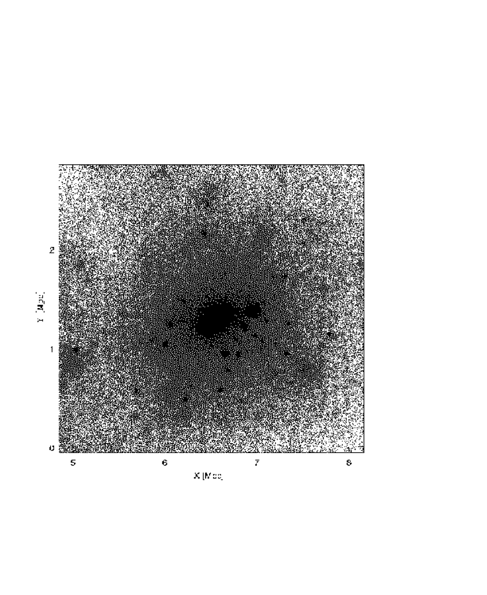
Figure 1: The simulated cluster used in our analysis. In gray we show all the mass particles in the simulation, in black the particles selected according to the criteria discussed in Section 2.

All the particles flagged by this procedure are shown in Figure 1, and they are overplotted to all the mass–particles in the simulation in the Virgo–like cluster region. These flagged particles provide us with a subsample of particles from the simulation, that have spent part of their lifes in the high-density region of at least one halo at $z>0.5$, and as previously argued, are good tracers of the baryons that formed stars in these dark halos. Then the division of the stellar component into galaxies or intracluster regions at $z=0$ can be easily achieved by selecting appropriate fields in the simulated data.

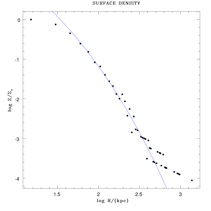
Figure 2: Surface density profile of the selected tracer particles in a cone free of surrounding subhalos, normalised to the central value, the full line shows an R^1/4 profile fitted to the inner parts. The outer profile indicates that the particle distribution there is not yet relaxed and some excess over the inner profile is present.

The surface density distribution of selected particles is shown in Figure 2. In producing this figure we have used particles in a cone which was free of obvious subhalo concentrations, so as to isolate the smooth component centred on the BCG. In the inner parts, this surface density profile follow closely an $r^{1/4}$ law; this result is similar to that of Dubinski (1998), which was based on a completely different treatment of the luminous component. The outer profile in Figure 2 shows the unrelaxed nature of the intracluster component at large radii, and suggests that after relaxation the density in these parts will have an excess of light in comparison with the $r^{1/4}$ law.

We have used a simple approach to identify luminous tracer particles through a density threshold criterion. As Figs. 1 and 2 show, this leads to a realistic stellar mass distribution. Because in cosmological dark matter halos with NFW profiles, relatively few stars in the densest regions come into the centre on elongated radial orbits from large distances, we expect that a selection based on binding energy would have produced largely similar results. We have also neglected the fact that part of the later intracluster material would be stripped from disks rather than spheroidal components. Material dispersed into intracluster space from cold components would be dynamically colder, even though it would have been typically heated by bar formation prior to stripping. Even stripped halos are still cold compared to the cluster velocity dispersion, however, so they also produce narrow structures in phase-space. Structures in phase-space originating from cold components would be even narrower, but not change our main results.

2.2 The conversion factor to ICPNe

Since we want to trace the properties of the ICSP and compare it with the ICPNe surveys, we need to define a conversion from the stellar-mass-particles in the N-body simulation to ICPNe, through the mass-to-light ratio of the stellar population. We assume that at $z=0$ the luminosity, mass-to-light ratio, etc., of the harassed–stellar matter are those of an evolved stellar population like those of M31.

This approach differs with respect to a semi–analytical approach because there is no Montecarlo realization of the baryonic population attached to the mass particles (see for example Kauffmann et al., 1994; Cole et al., 1994; Diaferio et al., 2001; Springel et al., 2001). All the information on the stellar population parameters that generate a PN in a galaxy environment is condensed in the luminosity-specific PN density, which specifies the number of PNe per unit luminosity. This quantity depends on the age and metallicity of a stellar population and it is a measured quantity. Here we adopt the luminosity-specific planetary nebulae density from M31: $\alpha_{1,B}=9.4\times 10^{-9}PNL_{B}^{-1}$ (Ciardullo et al., 1989). This is the best empirically determined value for an evolved population. $\alpha_{1,B}$ is the luminosity-specific planetary nebulae density within 1 mag from the bright cut-off of the planetary nebulae luminosity function (PNLF). We adopt this value because the ICPNe samples available in the literature are generally complete down to about 1 mag from the bright cut-off of their PNLFs.

The number of PNe per selected stellar–tracer mass particle (if not explicitly specified, we will refer to this selected stellar–tracer population as mass particles in what follows) in the cosmological simulation is then

$$n_{PN}/\mathrm{prtcl}=\frac{\alpha_{1,B}\times m_{p}}{\Gamma_{\mathrm{B}}}=\frac{9.4\times 10^{-9}\times 0.506\times 10^{9}}{\Gamma_{\mathrm{B}}}$$

where $m_{p}=0.506\times 10^{9}M_{\odot}$ is the mass of each mass particle in the simulation and $\Gamma_{\mathrm{B}}$ is a mass-to-light ratio, $\Gamma_{\mathrm{B}}$ = $M/L_{B}$, for the diffuse stellar population from which the ICPNe evolved. The best estimate for $\Gamma_{\mathrm{B}}$ is the value observed in galaxy regions where the dynamics is dominated by the luminous component alone. To be consistent with the adopted value of $\alpha_{1,B}$, we take the $\Gamma_{\mathrm{B}}$ value for the M31 bulge. Braun (1991) found $\Gamma_{\mathrm{B}}=6.5\pm 0.4$ for the bulge and disk of M31. With these assumptions, we obtain n${}_{PN}=0.74$ per mass particle, and n${}_{PN}=1$ is obtained for a $\Gamma_{\mathrm{B}}$ about 5. In what follows, we will adopt one PN for each mass particle after verifying that a $\Gamma_{\mathrm{B}}\sim 5-6$ is a consistent value for the ICSP.

2.3 Check on the stellar baryon fraction

An additional test on our selection of intracluster stars is whether the population we have chosen has a reasonable stellar baryon fraction in the selected IC fields. Once a ICSP is selected in an IC field, we take its mass to be the total stellar mass in this field, $M_{\mathrm{sel}}$. The stellar baryon fractions in this field is obtained by dividing $M_{\mathrm{sel}}$ by the total mass (dark+stellar), $M_{\mathrm{tot}}$, for all the mass particles in the same area. This is the compared with the corresponding number estimated for galaxy clusters.

Fukugita et al. (1998) found that the total contribution from stars in clusters, i.e. from spheroids, disks and irregular galaxies amounts to $\Omega_{\mathrm{stars}}=0.0027$, with an upper limit of about 0.005 and a minimum of about 0.0015 (for $h_{0}$=0.7) which, divided by $\Omega_{\mathrm{m}}=0.3$ (as in our simulation) gives a stellar baryon fraction ranging from 0.005 to 0.016 with a central value of $f_{\mathrm{stars}}=\Omega_{\mathrm{stars}}/\Omega_{\mathrm{m}}\sim$0.01. This is consistent with the recent estimate of the fraction of cluster baryons condensed in stars $f_{\mathrm{c,global}}=\Omega_{\mathrm{stars}}/\Omega_{\mathrm{bar}}=0.073h$ from Balogh et al. (2001). Following these authors in adopting $\Omega_{\mathrm{bar}}=0.039h^{-2}$ (Jaffe et al., 2001) and $\Omega_{\mathrm{m}}=0.3$, we obtain $f_{\mathrm{stars}}=0.0135$ (for $h_{0}$=0.7). We assume that the stellar baryon fraction does not differ greatly from this mean value at different positions in the cluster, and use this estimate in the intracluster fields discussed below.

3 Spatial and velocity structure of the ICSP population

3.1 Field selection and comparison strategy with ongoing surveys

We wish to use the simulated dataset at $z=0$ to predict those observables, the 2D distribution and the LOS velocity distribution, which can be readily compared with the results from photometric and spectroscopic ICPNe surveys. Photometric ICPNe sample are currently available (see Feldmeier et al., 1998; Arnaboldi et al., 2002, 2003; Ciardullo et al., 2002) and spectroscopic data may soon become so.

To facilitate a comparison with the ongoing surveys, we have chosen a series of projected regions in our data cube with the typical dimensions of the present wide-field-imaging cameras (WFI–like fields), 30${}^{\prime}\times$30^′, at different distances from the simulated Virgo–like cluster center. Assuming a distance of 15 Mpc for Virgo (as determined from the PNLF of M87), these WFI–like regions cover 0.131$\times$0.131 Mpc² in linear scale. These regions were selected at $R=0.2,~{}0.4,~{}0.5$ and 0.6 Mpc from the center, which corresponds to about $0.5,1,1.25\mbox{ and }1.5$ core radii respectively. These fields are placed so as to avoid significant sub–halos or overdensities which can be related to cluster galaxies.

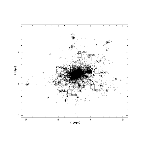
Figure 3: Here only the stellar tracers in the simulated cluster plus the fields adopted for the analysis are shown: CORE–like fields (top left), RCN1–like fields (top right), $F500$ fields (bottom left) and $F600$ fields (bottom right).

In what follows, we shall refer to CORE–like and RCN1–like for fields placed at $R$=0.2 Mpc and $R$=0.4 Mpc respectively (for similarity with the adopted convention in Arnaboldi et al. (2002) and Aguerri et al. (2003)). Fields at $R$=0.5 Mpc and $R$=0.6 Mpc will be named $F500$ and $F600$ respectively. In Figure 3, we show the fields selected at different distances from the cluster center. We have adopted the Z-axis as the line-of-sight and the X-Y plane as the plane of the sky, then we have analyzed for each field:
1) the M/L ratios (where information on the observed ICSP surface brightness is available from observations) and the baryonic stellar fraction as a check on the ICSP selection;
2) the 2D spatial distribution via the angular two-point correlation function (2PCF) using the Landy & Szalay (1993) estimator $\omega(\theta)$, as discussed in the Appendix;
3) the velocity distribution in order to evaluate the dynamical status of the ICSP:

3.2 Fields outside of the BCG halo (R$\geq$0.4 Mpc)

3.2.1 M/L ratios and baryonic stellar fraction

RCN1–like fields. The global properties of the selected fields are summarised in Table 1. We determined the M/L ratios for the RCN1-like fields in the simulations by computing the local surface mass densities from the selected ICSP particles and adopting the surface brightness from Arnaboldi et al. (2002). In most cases, resulting M/L ratios are compatible with an ICSP; fields 1RC3 and 1RC8 have larger M/L ratios than for a pure stellar population. Baryonic stellar fractions ($M_{\mathrm{sel}}/M_{\mathrm{tot}}$ in the fields, see Sect. 2.3) are shown in Table 1: they are in a range of 1-2% with a mean value of 0.015, in agreement with values observed in clusters.

$F500$ and $F600$ fields. The global properties of the selected fields are summarised in Table 2 and 3. We do not perform a check on the M/L ratios because we have no surface brightness (SB) information; no fields have been surveyed so far at such a large distances from the cluster center. The mean stellar baryonic fractions are 0.011 and 0.015 respectively, consistent with an ICSP population.

3.2.2 Velocity distributions

RCN1–like fields. Figure 4 shows the velocity distribution of the ICSP particles in some of these fields. The mean velocity, standard deviation, and kurtosis for these distributions along the three Cartesian axes are listed in Table 4. The inspection of Figure 4 shows clear deviations from a Gaussian distribution, as is also evident from the kurtosis analysis: the negative values of the kurtosis rule out a Gaussian distribution at the 95% c.l in at least one of the Cartesian coordinates, for the majority of the selected fields.

The non-Gaussian nature of the velocity distribution in Figure 4 signifies that the ICSP has only partially phase mixed. This is also seen from the lower panels of Figure 4 which show projections of the particle in the RCN1 fields onto two dimensional phase spaces. In these diagrams there are filaments, clusters of particles, and large empty regions. The dense clump in Field 1RCN6 comes from a local overdensity in the particle distribution which might be a separate small subsystem. The filaments probably originate from streams of particles which became unbound simultaneously and still have velocities well correlated with their positions. The voids are regions into which no such particle streams have yet phase mixed. It is possible that these diagrams even underestimate the amount of phase space substructures, because individual particle orbits are often not integrated accurately over long times in N-body codes.

$F500$ and $F600$ fields. Velocity distribution parameters are listed in Table 4. As for the RCN1–like fields, negative values of the kurtosis suggest a general deviation from a Gaussian distribution toward a flatter behavior even if it is not as strong as in case of the RCN1–like fields. In some cases, in the $F5004$, $F5009$, $F6006$ fields, the radial velocity distributions follow a Gaussian.

The unrelaxed, non-Gaussian nature of these velocity distributions shows that the ICSP has not had time to phase-mix on the scales probed. This is a strong prediction of this hierarchical cluster formation model, to be tested by future spectroscopic surveys.

3.2.3 2D spatial distribution

RCN1–like fields. Using the LS estimator, we label a field as clustered when its $\omega(\theta)$ differs significantly from zero given the errors. Results are listed in Table 5. The 2D clustering properties are anti–correlated with the degree of relaxation in the fields as derived by the velocity distributions: almost all fields that have a flat velocity distribution, in at least one direction, incompatible with a Gaussian distribution, are also clustered.

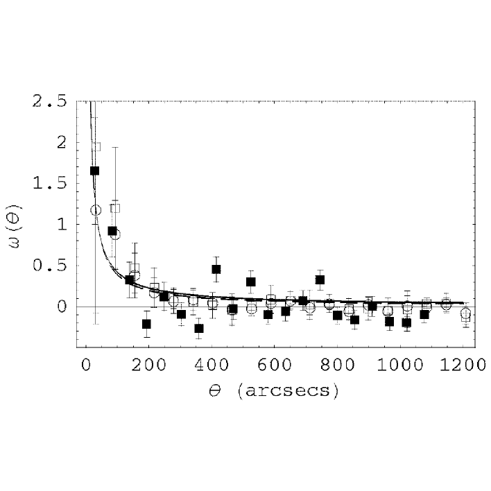
Figure 5: 2PCFs for the RCN1 fields. Open squares are the mean $\langle 2PCF\rangle$ from all the RCN1–like fields, open circles show the mean $\langle 2PCF\rangle$ with a (25%) contamination from a uniform population, filled squares are the 2PCF from the ICPNe data. Solid curve is the fit to open circles, dashed curve is the fit to the ICPNe sample: see discussion in the text.

The mean 2PCF over all fields is shown in Figure 5, where we compared it with that obtained from the RCN1 observed data (Aguerri et al., 2003). The 2PCF from the simulation shows a stronger clustering signal, i.e., it is systematically larger than the 2PCF from the observed RCN1 at small $\theta$: in particular the innermost bins have 1.5 times larger values in the simulated fields. Such an offset can be caused (see also Giavalisco et al., 1998) by the inferred 25% contamination by high-z emitters expected in the ICPNe catalogue (see Arnaboldi et al., 2002). In order to check this we have added a 25% uniform population to each of the simulated fields and computed again the mean 2PCF for the RCN1-like fields. The results are also given in Figure 5. The mean 2PCF from the simulation including the contamination, and the ICPN 2PCF are now compatible within the errors. The 2PCF fit to the power–law as in eq. A3 gives $A_{w}=25\pm 16$ and $\beta=0.89\pm 0.15$ for the average 2PCF from the simulation fields and $A_{w}=35\pm 20$, $\beta=0.98\pm 0.31$ from the photometrically complete sample of 55 ICPNe candidates (i.e. the sample selected within about 1 mag from the PNLF cutoff, see Aguerri et al., 2003, for further details): these values are fully consistent within the errors. We conclude that the observed RCN1 field has a clustering signal consistent with that expected from the N-body simulation.

$F500$ and $F600$ fields. No clear evidence for a clustering signal comes from the averaged 2PCF for both sets of fields (more marked for the $F600$ fields), except for a few $F500$ fields which are clustered.

3.3 CORE–like fields

In our simulated dataset, the BCG halo extends out to about 150 kpc from the galaxy center and it appears relaxed, with no evident spatial structures. At a distance of 15 Mpc, 150 kpc corresponds to about 34^′, i.e. the distance of the observed Core field from M87. Therefore fields selected at these radii in the simulated data cube will be embedded in the BCG extended halo. As discussed in Section 2.1, at high–z our adopted ICSP selection criteria also find DM particles. Thus in the extended BCG halo we expect a mix of stellar and DM tracers in our ICSP particle catalogue.

M/L ratios. Because of the substantial DM component in the model ICSP in the CORE–like fields, the computed $\Gamma_{\mathrm{B}}$ values (Table 6) are much larger than for a pure ICSP component.

The velocity distributions. The kurtosis values computed for the velocity distributions are shown in Table 4, together with the other parameters. Different from the RCN1–like fields, here negative kurtosis values are rare, and close to zero. The large mass-to-light ratios and the quasi-Gaussian velocity distributions indicate that the selected ICSP particles are more nearly relaxed (i.e., phase-mixed). Furthermore, some large positive kurtosis values ($>$1.2) suggest the presence of tails in the velocity distributions.

Is this a signature of an unrelaxed population as those observed in the fields further away from the BCG halo? In the BCG halo fields, given the setup of the simulation, we cannot say whether there is a relaxed ICSP component in addition to the DM particles, because we have no independent way of selecting it. If the ICSP is related to some unrelaxed population, however, then we can hope to select it via the identification of substructures in the velocity distribution. Given the large number of mass particles in the BCG halo fields, we can subtract the particles associated with a relaxed component and study the properties of the remaining particles.

This is done as follows. We make a Gaussian fit to the velocity distribution in each BCG halo field, and generate a “relaxed” population of particles whose radial velocities are randomly extracted from the fitted Gaussian distribution. This relaxed population is then subtracted off the simulated particle distribution in the CORE–like fields. The particles remaining after this procedure, if any, are taken as residual ICSP population. In each field, we have produced 30 random realizations for the relaxed population from the same Gaussian radial velocity distribution and look for the presence of an unrelaxed component in all the 30 residual fields. Hereafter we refer to this procedure as a statistical velocity subtraction (SVS).

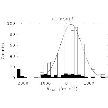
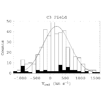
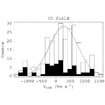
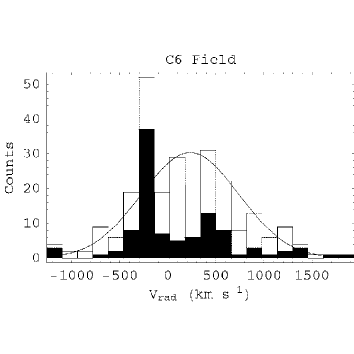
Figure 6: Results from the statistical velocity subtraction (SVS) for the CORE–like fields: velocity distributions of residual fields (black) in singular SVS experiments are overplotted on the velocity distributions for all the selected particles in different CORE–like fields.

Are the residual particle fields in the simulated CORE–like region compatible with the ICSP properties previously studied in the RCN1–like fields? Figure 6 shows a sample of these residual velocity fields; when an unrelaxed component is present the velocity distributions are similar to those from RCN1 fields. We can also verify whether the M/L ratio of this unrelaxed population is consistent with a M/L for a stellar population, and the results are shown in Table 7. The last row in this table lists the averaged quantities over all Core IC fields for the residual particles, after SVS. As a result, indeed the unrelaxed component is compatible with an ICSP population and the stellar baryon fraction, $\simeq 0.009$ in these fields is consistent with values expected for galaxy clusters.

3.3.1 Angular 2PCF

We compute the 2PCFs ($\omega(\theta)_{i}$, $i$=1…30) using the residual particle fields, then produce the mean $\langle\omega(\theta)\rangle$ and the relative error, given as the standard deviation of the $\omega(\theta)_{i}$ distribution. When the mean $\langle\omega(\theta)\rangle$ is compared with that computed for the all the particles in the fields the former has a clustering signal dominated by the DM particles, which show large clustering scales, while for the un-relaxed component the clustering scales are smaller, similar to those obtained for the RCN1–like fields.

We have performed several tests of the SVS procedure in order to identify systematic effects introduced by this approach, in particular, how a clustering signal would be modified after the SVS subtraction. As a test we have taken a RCN1–like field with significant clustering signal, and added a uniform distribution of particles, whose radial velocities where randomly extracted from a Gaussian with $\sigma=400$ kms^-1. We then applied the SVS, and compared the clustering signal in the residual particles with that in the original RCN1–like field. These tests indicate that the clustering signal is recovered correctly if the particles generating it are located in the tails of the velocity distribution, and that it is underestimated in the residual particles if the particles generating the signal are more uniformly spread over the velocity distribution. Applying the SVS procedure to the CORE-like fields will therefore not generate a spurious clustering signal.

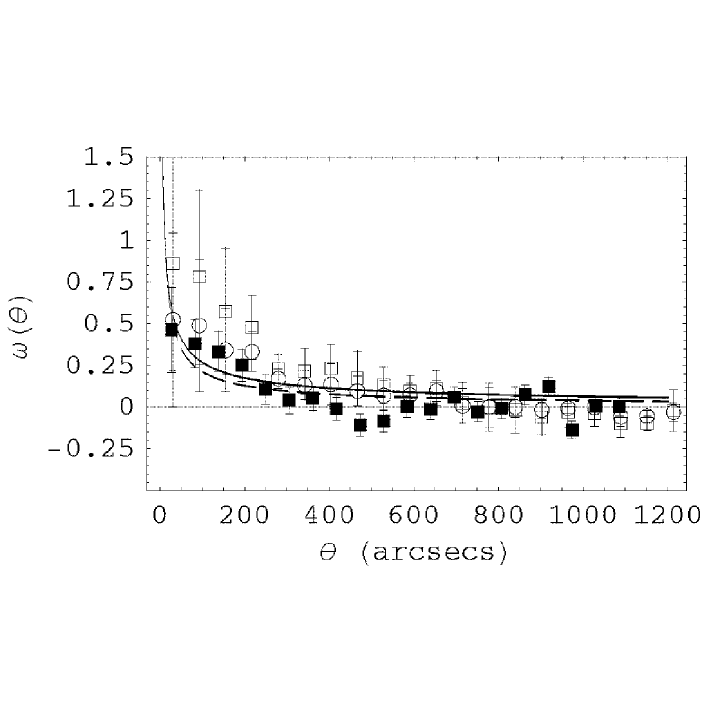
Figure 7: 2PCF for the Core fields. Symbol code as in Figure 5.

The mean 2PCF for the unrelaxed component plus a 25% uniform sample (see Sect 3.2.3) in the CORE–like simulation fields is shown in Figure 7, with the measured 2PCF from the observed ICPNe sample (77 candidates) superposed. The two are in agreement within the errors. The power law fit to the mean $\langle\omega(\theta)\rangle$ gives $A_{w}=5.2\pm 2.2$ and $\beta=0.62\pm 0.09$ from the simulated fields, and $A_{w}=6.1\pm 4.4$, $\beta=0.73\pm 0.18$ from the real data, considering the photometric complete sample of 77 ICPN candidates (see Aguerri et al., 2003). On the other hand, the mean 2PCF computed for all the particles in the CORE–like fields is not consistent with the measured 2PCF from the observed ICPN sample.

The results for the CORE–like fields are indicative of the properties of an un-relaxed stellar-like population in these regions. The inferred M/L ratios and the baryonic stellar fraction are compatible with an ICSP population at a distance of 0.2 Mpc from the cluster center. Furthermore the clustering properties of this un-relaxed ICSP population in the CORE-like regions are in agreement with those for the observed ICPN data in Virgo, at the same cluster radii.

4 Global properties of the ICSP

4.1 ICSP surface brightness and mass radial profiles at the cluster scales

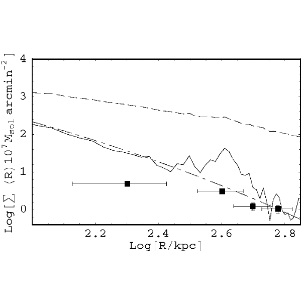
Figure 8: Radial surface density profiles for the ICSP. Surface brightness (SB) is on the upper panel: filled squares (triangles) are the mean SB values from the selected fields assuming $\Gamma_{\mathrm{B}}=5$ ($\Gamma_{\mathrm{B}}=6$), open squares are the estimates from the ICPNe data taking into account a 25% contaminants in the observed ICPNe data. Surface mass density (SM) is on the lower panel: filled squares are the mean SM values from the selected fields, continuous line show the total light (i.e. mass particles selected as stellar tracers) distribution, and dashed line is the total mass (luminous+dark).

Having selected an ICSP in our data cube of simulated particles, we can now predict its radial surface density profile and the results are shown in Figure 8. Here we compare the radial surface density profile from the ICSP component identified in the simulations with the points derived from the ICPN data. In the same Figure, we plot the surface mass density for all the dark particles in the simulation and for all the particles selected as stellar tracers (cf. Section 2). This comparison allows us to estimate the fraction of the mass associated with the ICSP in the simulation (i.e., the unrelaxed particles in the BCG halo fields and all the selected particles in the Intracluster fields), relative to the total stellar component. The distribution of the latter is averaged in annuli around the cluster center before comparing it with the ICSP surface mass density in the respective fields. We find that the ICSP component accounts for $\sim$33%, 29% and 50% of the total light in the RCN1–like, $F500$ and $F600$ fields respectively. For the CORE–like fields this estimate provides only a lower limit, because we cannot account for any relaxed stellar component, which may be present at these radii as well.

4.2 Clustering properties of the ICSP

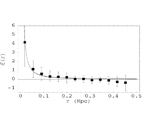
Figure 9: Average spatial 2-point correlation function from the RCN1-like fields from the simulated cluster. Error bars indicate 1 $\sigma$ confidence and solid line is the best-fit to the data. Discussion is in Section 4.2.

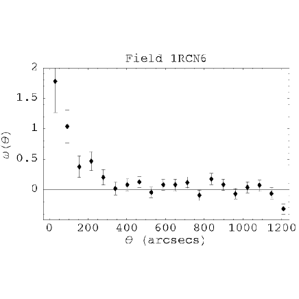
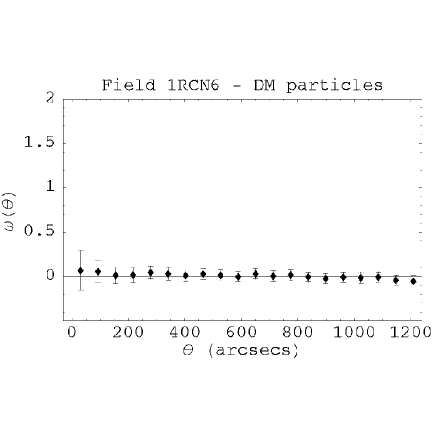
Figure 10: Observable properties of the selected stellar tracers (upper plots) vs. properties of the DM particles (lower plots) in the 1RCN6 field. Left panels: angular 2PCF; right panels: velocity distributions along the three Cartesian axes. The DM particles are relaxed and unclustered in the surveyed area, while the ICSP is clustered and unrelaxed.

In Figures 9 we show the average spatial 2PCF $\xi(r)$ for the RCN1–like fields: it indicates the presence of sub-structures in the ICSP. Similar features are found also in $F500$ and $F600$ fields. This evidence is stronger when we compare the clustering properties of the selected particles with those of the DM particles in the same field; in Figure 10 we show that there is no structure in the DM distribution as $\omega(\theta)$ is zero on all scales. A major result of this work is that the substructures in the ICSP are also evident in the radial velocity distribution of the ICSP particles in these IC fields, while the DM particles follow a Gaussian distribution as shown in Figure 10. From a Kolmogorov-Smirnov test, the velocity distributions for the ICPS and DM have less than 0.001 probability to come from the same distribution.

4.3 The degree of relaxation and density environment of the selected particles

An intriguing result from our analysis is that those particles identified as ICSP tracers are mostly unrelaxed in the velocity distribution. The most likely interpretation is that phase-mixing did not act for long enough to erase streamers or tails produced during galaxy interactions within the cluster. If a stream is produced during encounters, this will live for a period of order several dynamical times, $t_{\mathrm{dyn}}$. This is a function of the mass density at the location where the ICSP is evolving and is given by

$$t_{\mathrm{dyn}}=\sqrt{\frac{3\pi}{16G\rho}}$$ (1)

from Binney & Tremaine (1987), where $\rho$ is the mean density enclosed within the field distance from the center. Taking a mean of the selected fields at different distances we obtain $t_{\mathrm{dyn}}=(0.3,0.9,1.2,1.7)\times 10^{9}$ yr for fields at $R=(0.2,0.4,0.5,0.6)$ Mpc respectively. Phase-mixing timescales are thus of the order of several gigayears.

In this picture, both the degree of clustering and the velocity distribution of the ICSP particles give information on the history and evolution of the ICSP population. Because time scales for phase–mixing are large in cluster environments, it is difficult, however, to constrain the formation epoch from such streamers or tails. Perhaps more reliable constraints on the formation epoch for these structures may be obtained from the clustering properties which can be parametrised. Using the spatial 2PCF it is possible to derive the correlation scales for structures in the ICSP. The parameters for the best fit of Equation A4 to the $\xi(r)$ from RCN1–like, F$500$ and F$600$ fields as in Figure 9, are summarised in Table 8. Here $\gamma$ changes to lower values from the RCN1–like fields to the $F500$ fields, while the clustering radius $r_{0}$ becomes larger from RCN1–like to F500 fields. In the more distant $F600$ fields the clustering is quite weak and only present at smaller scales, as expected for populations of old streams for which the phase–mixing has erased the larger-scale structures. This suggests different dynamical evolution at different radii.

In the inner regions (R$\leq 0.4$ Mpc), the effects of these processes are evident. Here we are observing young ICSP clumps because the encounter probability is higher than at larger radii and structures are formed by harassment with higher frequency, and they are still unrelaxed and clustered. For structures originating more or less at the same epochs, the shorter dynamical time ($t_{\mathrm{dyn}}^{\mathrm{0.2}}/t_{\mathrm{dyn}}^{\mathrm{0.4}}=0.37$) in the BCG regions decrease the clustering signal with respect to structures forming at R=0.4 Mpc.

These estimates of $r_{0}$ are of the same order of magnitude as for the structures expected from harassment and tidal interaction in clusters (Gavazzi et al., 2001; Moore et al., 1996, 1998, 1999a).

The ICSP predicted in a hierarchical scenario for galaxy cluster formation is generally arranged in unrelaxed structures whose evolution is different from that of the stellar population condensed in galaxies. We have shown that the study of the velocity distributions can be used to distinguish older from younger streams. Constraints on the formation epoch of such a population also come from the clustering properties in the 2D distribution, for which observational data is now becoming available. Here younger streams are clearly identified as those with a significant clustering signal with respect to older streams for which clustering was erased by the random motions and phase-mixing.

5 Conclusions

We have used an N-body cosmological simulation in a $\Lambda$CDM cosmology to predict the properties of the intracluster stellar population (ICSP) in nearby galaxy clusters. We have selected particles from the simulation that trace the stellar component, by applying a density threshold criterion for redshifts $z\geq 0.5$. We have then focussed on the ICSP at $z=0$, by considering only “intracluster” fields in the model cluster, i.e., outside the central BCG galaxy and other cluster galaxies. The particles analysed in these fields are those that were lost from the inner halos they once belonged to at higher redshifts.

We have then studied the two-dimensional spatial distribution of this ICSP, comparing to existing data for the Virgo intracluster planetary nebulae (ICPNe). We have considered the two-point angular correlation function (2PCF) as a measure for the past dynamical evolution of the ICSP component. A significant clustering signal is expected if this component formed relatively recently without having time to phase-mix until the present, depending thus on the dynamical time on the different scales. The strongest clustering signal is found in the inner regions of the cluster ($R\leq 0.4{\rm Mpc}$) where the encounter probability appears to be largest. From the spatial 2PCF, we find a correlation length of 50 kpc at R=400–500 kpc in the simulation. The degree of clustering seen in the N-body ICSP is in approximate agreement with that inferred from the observed ICPNe dataset for the Virgo cluster.

The line-of-sight velocity distributions of the ICSP particles in the N-body model in intracluster fields are strongly non-Gaussian, consisting often of several distinct components, which trace the dynamical formation of the ICSP. Two-dimensional phase space diagrams show filaments, clusters of particles, and large empty regions, all of which indicate a young dynamical age. This is consistent with the model ICSP being in part made of particle streams as expected in a harassment picture. A strong prediction of this work is that, if the observed intracluster stars in the Virgo cluster formed in a similar way as in this N-body model, their velocity distributions should be highly non-Gaussian, and their phase space diagrams strongly unrelaxed, with subcomponents that should be easily observable in wide-field spectroscopic surveys of ICPNe.

Our results support the picture that the properties of the observed ICSP in the Virgo cluster are consistent with the hierarchical formation of cosmic structures and, more specifically, a complex and prolonged phase of galaxy infall into clusters. In future, we will have larger photometric and spectroscopic ICPNe data samples to measure the spatial and velocity substructure of the ICSP, and more refined simulations, following in detail the origin from individual harrassment events, and possibly including an explicit description of the star formation processes. This will allow us to compare in detail the internal structure of nearby galaxy clusters with cosmological cluster formation models, and use the properties of the ICSP to test the cosmological simulations and to constrain the cluster formation epoch.

Appendix A Clustering via angular two–point correlation function

Correlations in the distribution of a sample of objects offer, perhaps, the simplest and least ambiguous statistical description of their clustering properties. The angular correlation function, $w(\theta)$, is the projection of the spatial function on the sky and is defined in terms of the joint probability, $\delta P$, of finding two points separated by an angular distance $\theta$ relative to that expected for a random distribution Peebles (1980),

$$\delta P=N^{2}[1+w(\theta)]\delta\Omega_{1}\delta\Omega_{2},$$ (A1)

where $\delta\Omega_{1}$ and $\delta\Omega_{2}$ are elements of solid angle and $N$ is the mean number density of objects. For an unclustered population $w(\theta)=0$, while positive or negative values of $w(\theta)=0$ indicate clustering or anti-clustering respectively. Estimators for $w(\theta)$ are generally constructed out of ratios between three fundamental quantities. These are the number of pairs of objects (DD), the number of pairs given a cross–correlation between the points and a random distribution (DR), and the number of pairs for a random distribution (RR), all suitably normalized and accounting for the geometry of the fields where candidates were selected.

We have used the estimator proposed by Landy & Szalay (1993):

$$w(\theta)=\frac{DD(\theta)-2DR(\theta)+RR(\theta)}{RR(\theta)}.$$ (A2)

The Landy & Szalay estimator is a robust estimator because it removes edge effects for a field of arbitrary geometry, and gives a variance which is equivalent to Poissonian for an uncorrelated distribution of points. The angular two-point correlation function $w(\theta)$ can be represented by a power-law

$$w(\theta)=A_{w}\theta^{-\beta}$$ (A3)

(Giavalisco et al., 1998). If the spatial correlation function can be modeled as

$$\xi(r)=(r/r_{0})^{-\gamma}\times f(z)$$ (A4)

($f(z)=1$ for $z\sim 0$), the angular correlation function has, in fact, the form as in eq. A3, where $\beta=\gamma-1$ and $r_{0}$ is a characteristic clustering radius.

Figure 4: Velocity distributions and projected phase space diagrams for the ICSP in four RCN1–like fields. From top to botton: velocity distributions in transverse velocities on the sky, $V_{x}$ and $V_{y}$, and in line-of-sight velocity $V_{z}$; projected phase-space diagrams (R,$V_{z}$), ($x$,$V_{z}$), and ($y$,$V_{z}$), where R$=\sqrt{x^{2}+y^{2}}$.

Table 1: RCN1–like fields. (R,$\Phi$) are the polar coordinates in the sky plane, n.p.=number of particles(=ICPNe) selected in the fields, $M_{t}$= total mass of the particles in the fields, $f_{\mathrm{bar}}$ is the stellar baryon fraction in the selected fields. (*) $\Gamma_{\mathrm{B}}$ is obtained using the estimated surface brightness associated with the ICPNe, i.e. 6.2$\times 10^{6}$ $L_{\odot_{B}}$ arcmin^-2.

Field	R (Mpc)	$\Phi$(degrees)	n.p.	$M_{t}(10^{10}M\odot)$	$\Gamma_{\mathrm{B}}^{(*)}$	$f_{\mathrm{bar}}$
1RC1	0.4	60	57	2.885	5.1	0.014
1RC2	0.4	95	41	2.075	3.7	0.012
1RC3	0.4	220	137	6.93	12.4	N/A
1RC4	0.4	255	55	2.783	5.0	0.014
1RC5	0.4	315	68	3.441	6.1	0.022
1RC6	0.4	350	58	2.935	5.2	0.015
1RC7	0.4	143	49	2.48	4.4	0.013
1RC8	0.4	166	143	7.237	12.9	N/A

Table 2: $F500$ fields. (R,$\Phi$) are the polar coordinates in the sky plane, n.p.=number of particles(=ICPNe) selected in the fields, $M_{t}$= total mass of the particles in the fields.

Field	R (Mpc)	$\Phi$(degrees)	n.p.	$M_{t}(10^{10}M\odot)$
$F500$1	0.5	45	25	1.265
$F500$2	0.5	60	21	1.063
$F500$3	0.5	95	17	0.860
$F500$4	0.5	140	21	1.067
$F500$5	0.5	210	69	3.492
$F500$6	0.5	240	25	1.265
$F500$7	0.5	269	26	1.316
$F500$8	0.5	310	20	1.012
$F500$8	0.5	345	21	1.067

Table 3: $F600$ fields. (R,$\Phi$) are the polar coordinates in the sky plane, n.p.=number of particles(=ICPNe) selected in the fields, $M_{t}$= total mass of the particles in the fields.

Field	R (Mpc)	$\Phi$(degrees)	n.p.	$M_{t}(10^{10}M\odot)$
$F600$1	0.6	55	12	0.607
$F600$2	0.6	86	16	0.810
$F600$3	0.6	170	17	0.860
$F600$4	0.6	225	25	1.265
$F600$5	0.6	245	16	0.962
$F600$6	0.6	330	21	1.063
$F600$7	0.6	360	22	1.113

Table 4: Velocity moments along the three Cartesian axes for the selected fields: mean velocity ($\overline{v_{\mathrm{i}}}$), velocity dispersion ($\sigma_{\mathrm{i}}$) and kurtosis ($k_{\mathrm{i}}$) values (i=$x,y,z$).

Field	$\overline{v_{x}}$ (km s-1)	$\sigma_{x}$ (km s-1)	$k_{x}$	$\overline{v_{y}}$ (km s-1)	$\sigma_{y}$ (km s-1)	$k_{y}$	$\overline{v_{z}}$ (km s-1)	$\sigma_{z}$ (km s-1)	$k_{z}$
1RC1	80	401	-0.95	-181	549	-0.82	-366	524	0.91
1RC2	279	259	-0.58	117	388	0.11	436	553	-0.31
1RC3	96	447	-0.54	-18	471	-0.95	240	436	-0.46
1RC4	41	313	0.70	202	405	-1.05	199	399	0.7
1RC5	-274	477	3.40	140	397	0.84	-16	333	0.52
1RC6	51	695	1.46	242	414	0.65	-49	479	-1.17
1RC7	-23	327	-0.80	98	428	-0.22	5	384	-0.50
1RC8	50	449	-0.64	-6	258	-0.19	150	408	0.5
$F500$1	97	401	-1.02	-93	301	2.03	91	322	1.00
$F500$2	-119	268	-1.36	-387	333	-0.32	-35	182	1.45
$F500$3	200	194	0.12	0	476	-0.77	911	501	-1.53
$F500$4	30	384	2.59	125	255	-0.08	-232	266	0.67
$F500$5	56	509	-0.06	-26	402	-0.11	231	373	-0.22
$F500$6	178	254	-0.92	-28	674	-1.06	244	419	-1.43
$F500$7	27	280	-1.67	-78	444	-1.24	-304	745	-1.5
$F500$8	-215	389	-0.44	125	204	1.08	-1	263	2.54
$F500$9	100	441	1.46	-68	436	0.37	187	321	1.47
$F600$1	-16	154	-1.03	-18	203	-0.20	-337	336	-0.44
$F600$2	337	165	-0.36	-300	605	-0.78	316	367	2.62
$F600$3	395	681	-0.45	122	358	4.96	366	561	-1.37
$F600$4	-32	247	-0.07	-109	321	-0.95	51	360	-1.53
$F600$5	163	219	5.39	141	409	-0.53	372	186	0.89
$F600$6	-95	428	1.10	38	235	0.30	116	236	2.77
$F600$7	894	677	-0.54	53	209	0.35	44	277	-0.12
C1	122	474	2.5	151	459	0.09	107	643	0.09
C2	127	551	1.21	114	603	0.28	122	540	0.28
C3	173	401	3.92	117	534	-0.35	161	522	-0.35
C4	42	424	1.57	87	480	0.39	185	568	0.39
C5	24	432	1.21	127	541	-0.19	221	591	-0.19
C6	-2	605	-0.33	230	419	0.24	162	555	0.24
C7	301	767	0.63	172	336	1.98	121	455	1.98

Table 5: Clustering of the RCN1-like fields.

Field	CLASS
1RC1	clustered
1RC2	clustered
1RC3	clustered
1RC4	clustered
1RC5	clustered
1RC6	clustered
1RC7	not clustered
1RC8	not clustered

Table 6: CORE–like fields. (R,$\Phi$) are the polar coordinates in the sky plane, n.p.=number of particles(=ICPNe) selected in the fields, $M_{t}$= total mass of the particles in the fields. (*) $\Gamma_{\mathrm{B}}$ is obtained using the estimated surface brightness associated with the ICPNe, i.e. 9.7$\times 10^{6}$ $L_{\odot_{B}}$ arcmin^-2.

Field	R (Mpc)	$\Phi$(degrees)	n.p.	$M_{t}(10^{11}M\odot)$	$\Gamma_{\mathrm{B}}^{(*)}$
C1	0.2	140	872	4.413	51.2
C2	0.2	70	535	2.707	31.4
C3	0.2	105	434	2.196	25.5
C4	0.2	240	734	3.7145	43.1
C5	0.2	280	257	1.3001	15.1
C6	0.2	310	259	1.3107	15.2
C7	0.2	7	754	3.8156	44.3

Table 7: Results for CORE–like fields, after the SVS. $\langle V\rangle$=mean and SD= standard deviation of the gaussian fits; a.n.p.= the average number of objected selected in the SVS (over 30 experiments). Last row are the mean values over the six fields. (*) $\Gamma_{\mathrm{B}}$ is obtained using the estimated surface brightness associated with the ICPNe, i.e. 9.7$\times 10^{6}$ $L_{\odot_{B}}$ arcmin^-2.

Field	$\langle V\rangle$	SD	a.n.p.	$M_{t}(10^{10}M\odot)$	$\Gamma_{\mathrm{B}}^{(*)}$
C1	206	483	93	4.710	5.5
C2	232	421	94	4.757	5.5
C3	211	452	71	3.593	4.2
C4	205	488	99	5.010	5.8
C5	271	491	67	3.391	4.0
C6	232	515	96	4.858	5.6
$\langle C\rangle$			87	4.387	5.0

Table 8: Mean spatial 2PCF outside the cD halo: parameters of the fits with 1 $\sigma$ errors.

Field	$\gamma$	$r_{0}(kpc)$
RCN1	$1.49\pm 0.16$	$50\pm 5$
$F500$	$1.35\pm 0.18$	$58\pm 7$
$F600$	$1.8\pm 0.9$	$30\pm 10$

References

- Aguerri et al. (2003) Aguerri L., J.A. et al. 2003, in preparation
- Arnaboldi et al. (1996) Arnaboldi, M., et al. 1996, ApJ, 472, 145
- Arnaboldi et al. (2002) Arnaboldi, M., Aguerri L., J.A., Napolitano, N.R., et al. 2002, AJ, 123, 760
- Arnaboldi et al. (2003) Arnaboldi, M., et al. 2003, AJ, 125, 514
- Balogh et al. (2001) Balogh, M.L., Pearce, F.R., Bower, R.G., & Kay, S.T. 2001, MNRAS, 326, 1228
- Binney & Tremaine (1987) Binney, J.J., & Tremaine, S. 1987, Galactic Dynamics, Princeton Series in Astrophysics
- Borgani et al. (2001) Borgani, S., Governato, F., Wadsley, J., Menci, N., Tozzi, P., Lake, G., Quinn, T., & Stadel, J. 2001, ApJ, 559, L71
- Braun (1991) Braun, R. 1991, AJ, 372, 54
- Bullock et al. (2001) Bullock, J.S., Kolatt, T.S., Sigad, Y., Somerville, R.S., Kravtsov, A.V., Klypin, A.A., Primack, J.R., & Dekel, A. 2001, MNRAS, 321, 559
- Calcáneo-Roldán et al. (2000) Calcáneo-Roldán,C., Moore, B., Bland-Hawthorn, J., Malin, D., & Sadler, E.M. 2000, MNRAS, 314, 324
- Ciardullo et al. (1989) Ciardullo, R., Jacoby, G.H., Ford, H.C., & Neill, J.D. 1989, ApJ, 339, 53
- Ciardullo et al. (1998) Ciardullo, R., Jacoby, G.H., Feldmeier, J.J., & Bartlett, R.E. 1998, ApJ, 492, 62
- Ciardullo et al. (2002) Ciardullo, R., Feldmeier, J.J., Krelove, K., Jacoby, G.H., & Gronwall, C. 2002, ApJ, 566, 784
- Cole et al. (1994) Cole, S., Aragon-Salamanca, A., Frenk, C.S., Navarro, J.F., & Zepf, S.E. 1994, MNRAS, 271, 781
- Diaferio et al. (2001) Diaferio, A., Kauffmann, G., Balogh, M.L., White, S.D.M., Schade, D., & Ellingson, E. 2001, MNRAS, 323, 999
- Dubinski (1998) Dubinski, J., 1998, ApJ, 502, 141
- Feldmeier et al. (1998) Feldmeier, J.J., Ciardullo, R., & Jacoby, G.H. 1998, ApJ, 503, 109
- Feldmeier et al. (2002) Feldmeier, J.J., Mihos, J.C., Morrison, H.L., Rodney, S.A., & Harding, P. 2002, ApJ, 575, 779
- Fukugita et al. (1998) Fukugita, M., Hogan, C.J., & Peebles, P.J.E. 1998, ApJ, 503, 518
- Gavazzi et al. (2001) Gavazzi, G., Boselli, A., Mayer, L., Iglesias-Paramo, J., Vílchez, J.M., Carrasco, L. 2001, ApJ, 563, L23
- Giavalisco et al. (1998) Giavalisco, M., Steidel, C.C., Adelberger, K.L., Dickinson, M.E., Pettini, M., & Kellogg, M. 1998, ApJ, 503, 543
- Governato et al. (1998) Governato, F., Baugh, C.M., Frenk, C.S., Cole, S., Lacey, C. G., Quinn, T., & Stadel, J. 1998, Nature, 392, 359
- Governato et al. (2001) Governato, F., Ghigna, S., Moore, B., Quinn, T., Stadel, J., & Lake, G. 2001, ApJ, 547, 555
- Governato, Ghigna & Moore (2001) Governato, F., Ghigna, S., & Moore, B. 2001, ASP Conf. Ser. 245: Astrophysical Ages and Times Scales, 469
- Guiderdoni et al. (1998) Guiderdoni, B., Hivon, E., Bouchet, F.R., & Maffei, B. 1998, MNRAS, 295, 877
- Helmi (2001) Helmi, A. 2001, Nature, 412, 25
- Katz & White (1993) Katz, N. & White, S.D.M. 1993, ApJ, 412, 455
- Kauffmann et al. (1994) Kauffmann, G., Guiderdoni, B., & White, S.D.M. 1994, MNRAS, 267, 981
- Jaffe et al. (2001) Jaffe, A.H., et al. 2001, Phys. Rev. Lett., 86, 3475
- Landy & Szalay (1993) Landy, S.D. & Szalay, A.S. 1993, ApJ, 412, L64
- Mayer et al. (2001) Mayer, L., Governato, F., Colpi, M., Moore, B., Quinn, T., Wadsley, J., Stadel, J., & Lake, G. 2001, ApJ, 547, L123
- Merritt (1984) Merritt, D. 1984, ApJ, 276, 26
- Mo et al. (1998) Mo, H.J., Mao, S., & White, S.D.M. 1998, MNRAS, 295, 319
- Moore et al. (1996) Moore, B., Katz, N., Lake, G., Dressler, A., & Oemler, A.Jr. 1996, Nature, 379, 613
- Moore et al. (1998) Moore, B., Lake, G., & Katz, N. 1998, ApJ, 495, 139
- Moore et al. (1999a) Moore, B., Lake, G., Quinn, T., & Stadel, J. 1999a, MNRAS, 304, 465
- Moore et al. (1999b) Moore, B., Ghigna, S., Governato, F., Lake, G., Quinn, T., Stadel, J., & Tozzi, P. 1999b, ApJ, 524, L19
- Navarro et al. (1997) Navarro, J.F., Frenk, C.S., & White, S.D.M. 1997, ApJ, 490, 493
- Nelson et al. (2002) Nelson, A.E., Simard, L., Zaritsky, D., Dalcanton, J.J., & Gonzalez, A.H. 2002, ApJ, 567, 144
- Okamura et al. (2002) Okamura, S., et al., 2002, PASJ, 54, 883
- Peebles (1980) Peebles, P. J. E. 1980, The Large scale structure of te Universe (Princeton: Princeton Univ. Press)
- Simard et al. (1999) Simard, L., et al. 1999, ApJ, 519, 563
- Springel et al. (2001) Springel, V., White, S.D.M., Tormen, G., & Kauffmann, G. 2001, MNRAS, 328, 726
- Theuns & Warren (1997) Theuns, T., & Warren, S. 1997, MNRAS, 284, L11
- van den Bosch (2000) van den Bosch, F.C. 2000, ApJ, 530, 177
- Wechsler et al. (2002) Wechsler, R.H., Bullock, J.S., Primack, J.R., Kravtsov, A.V., & Dekel, A. 2002, ApJ, 568, 52
- White & Rees (1978) White, S.D.M. & Rees, M.J. 1978, MNRAS, 183, 341
- Zhao et al. (2002) Zhao, D.H., Mo, H.J., Jing, Y.P., & Boerner, G. 2002, MNRAS, 339, 12