Ordinary and Viscosity-Damped MHD Turbulence

Abstract

We compare the properties of ordinary strong magnetohydrodynamic (MHD) turbulence in a strongly magnetized medium with the recently discovered viscosity-damped regime. We focus on energy spectra, anisotropy, and intermittency. Our most surprising conclusion is that in ordinary strong MHD turbulence the velocity and magnetic fields show different high-order structure function scalings. Moreover this scaling depends on whether the intermittency is viewed in a global or local system of reference. This reconciles seemingly contradictory earlier results. On the other hand, the intermittency scaling for viscosity-damped turbulence is very different, and difficult to understand in terms of the usual phenomenological models for intermittency in turbulence. Our remaining results are in reasonable agreement with expectations. First, we find that our high resolution simulations for ordinary MHD turbulence show that the energy spectra are compatible with a Kolmogorov spectrum, while viscosity-damped turbulence shows a shallow $k^{-1}$ spectrum for the magnetic fluctuations. Second, a new numerical technique confirms that ordinary MHD turbulence exhibits Goldreich-Sridhar type anisotropy, while viscosity-damped MHD turbulence shows extremely anisotropic eddy structures. Finally, we show that many properties of incompressible turbulence for both the ordinary and viscosity-damped regimes carry over to the case of compressible turbulence.

1 Introduction

The interstellar medium (ISM) shows density and velocity statistics that indicate the existence of strong turbulence (Armstrong, Rickett, & Spangler 1995; Lazarian & Pogosyan 2000; Stanimirovic & Lazarian 2001; see also the review by Cho, Lazarian, & Vishniac 2003 and references therein). Understanding interstellar turbulence is essential for many astrophysical processes including star formation, and cosmic ray transport (see reviews by Vazquez-Semadeni et al. 2000; Lazarian, Cho, Yan 2002 and references therein). Moreover, the importance of magnetohydrodynamic (MHD) turbulence is not limited to interstellar processes. For instance, properties of MHD turbulence may be essential for describing gamma ray bursts (see Lazarian et al. 2003) and magnetic reconnection (Lazarian & Vishniac 1999).

Kolmogorov theory (1941) is the simplest model for incompressible hydrodynamic turbulence. The main prediction of the theory is the velocity-separation relation $v_{l}\sim l^{1/3}$, or energy spectrum $E(k)\sim k^{-5/3}$, where $l$ is the separation between two points (or, we regard it as eddy size) and $k\sim 1/l$ is the wave number. In general, $kE(k)\sim v_{l}^{2}$. Astrophysical turbulence differs from its laboratory counterpart in that it is usually magnetized, compressible, and the gas can be partially ionized. However, the single most important difference is that typical large eddy scales in MHD turbulence are usually many orders of magnitude larger than any relevant microphysical scale. This allows us to sidestep many of the issues that make laboratory plasma physics so complicated.

Including magnetic field effects has a dramatic effect on strong turbulence. Our current understanding of MHD turbulence owes a great deal to fundamental results obtained by Shebalin, Matthaeus, & Montgomery (1983), Higdon (1984), Matthaeus et al. (1998) and other researchers (see a more complete list in Cho, Lazarian & Vishniac 2003). Recently Goldreich & Sridhar (1995; hereafter GS95) proposed a model for incompressible MHD turbulence, which was later supported by numerical simulations (Cho & Vishniac 2000; Maron & Goldreich 2001). The GS95 model predicts a Kolmogorov energy spectrum, $E(k)\sim k^{-5/3}$, for both velocity and magnetic fields. The major difference between MHD and hydrodynamic turbulence is the anisotropy of the eddy structures - eddies are statistically isotropic in hydrodynamic turbulence while eddies show scale-dependent anisotropy (i.e. smaller eddies are more anisotropic) in the MHD case (see Cho, Lazarian, & Vishniac 2003).

How useful is studying incompressible turbulence? Does it have anything to do with turbulence in realistic compressible flows? Compressible MHD turbulence has been studied intensively by different researchers (for a review see Cho & Lazarian 2003c and references therein). A discussion of the extent to which the incompressible GS95 scaling is applicable to realistic compressible fluids may be found in the original GS95 paper. More recently Lithwick & Goldreich (2001) extended GS95 model for high-$\beta$ ($\beta\equiv P_{gas}/P_{magnetic}$) plasmas, i.e. for the case when gas pressure is larger than magnetic pressure. They also made a conjecture about the scaling of slow modes in low-$\beta$ plasmas. Cho & Lazarian (2002) studied turbulence in low-$\beta$ plasmas and obtained numerical scaling relations for both compressible and Alfvenic modes. Finally, both the high- and low-$\beta$ plasma cases are covered in Cho & Lazarian (2003a,b). They showed that the Alfvenic and slow modes follow the GS95 scaling not only for Mach numbers much less than unity, but also for much larger Mach numbers, as long as the motions were still sub-Alfvenic. Fast modes were shown to be decoupled from the rest of the modes and isotropic. The work on compressible turbulence shows that incompressible simulations are meaningful in terms of representing most features of realistic flows. Consequently in this paper we concentrate on incompressible turbulence.

In this paper, we focus on the effects of viscosity. In strong hydrodynamic turbulence energy is injected at a scale $L$, and cascades down to smaller scales without significant viscous losses until it reaches the viscous damping scale $l_{dv}$. The Kolmogorov energy spectrum applies to the inertial range, i.e. all scales between $L$ and $l_{dv}$. This simple picture becomes more complicated when we deal with MHD turbulence because there are two dissipation scales - the velocity damping scale $l_{dv}$ and the magnetic diffusion scale $l_{dm}$, where magnetic structures are dissipated. In fully ionized collisionless plasmas (e.g. the hottest phases of the ISM), $l_{dv}$ is less than an order of magnitude larger than $l_{dm}$, but both scales are very small. However, in partially ionized plasmas (e.g. the warm or cold neutral phase of the ISM), the two dissipation scales are very different and $l_{dv}\gg l_{dm}$. In the Cold Neutral Medium (see Draine & Lazarian 1999 for a list of the idealized phases) neutral particle transport leads to viscous damping on a scale which is a fraction of a parsec. In contrast, in these same phases $l_{dm}\sim 100km$.

This has a dramatic effect on the energy cascade model in a partially ionized medium. When the energy reaches the viscous damping scale $l_{dv}$, kinetic energy will dissipate there, but the magnetic energy will not. In the presence of dynamically important magnetic field, Cho, Lazarian, & Vishniac (2002b; hereafter CLV02b) reported a completely new regime of turbulence below the scale at which viscosity damps kinetic motions of fluids. They showed that magnetic fluctuations extend below the viscous damping scale and form a shallow spectrum $E_{b}(k)\sim k^{-1}$. The spectrum is similar to that of the viscous-convective range of a passive scalar in hydrodynamic turbulence (see, for example, Lesieur 1990). In addition they showed that turbulence in the new regime is very anisotropic and intermittent. Here, we compare ordinary and viscosity-damped MHD turbulence. We mainly focus on the energy spectra, eddy anisotropy, scale-dependent intermittency, and intermittency from high order velocity statistics.

In what follows, we briefly consider a theoretical model for viscosity-damped turbulence (§2). A detailed theoretical study is given in Lazarian, Vishniac & Cho (2003; hereafter LVC03). We discuss our numerical method in §3. We present our results on anisotropies and intermittency in §4, while results on higher-order statistics are given in §5. A discussion and the summary are presented in §6 and §7 respectively.

2 A Theoretical Model for Viscosity-Damped MHD Turbulence

Following the usual treatment of ordinary strong MHD turbulence, we define the wavenumbers $k_{\|}$ and $k_{\perp}$ as the components of the wavevector measured along the local mean magnetic field and perpendicular to it, respectively. In this Here the local mean magnetic field is the direction of the locally averaged magnetic field, which depends not only on the location but also the volume over which the average is taken. See Cho & Vishniac (2000) and Cho, Lazarian, & Vishniac (2002a; hereafter CLV02a) for details.

Lazarian, Vishniac, & Cho (LVC03) proposed a theoretical model for viscosity-damped MHD turbulence. We summarize the model as follows.

Since there is no significant velocity fluctuation below $l_{dv}$, the time scale for the energy cascade below $l_{dv}$ is fixed at the viscous damping scale. Consequently the energy cascade time scale $t_{cas}$ is scale-independent below $l_{dv}$ and the requirement for a scale independent energy rate rate $b_{l}^{2}/t_{cas}$ yields

$$b_{l}\sim\mbox{constant, or~{}~{}~{}}E_{b}(k)\sim k^{-1},$$ (1)

where $kE_{b}(k)\sim b_{l}^{2}$.

In LVC03, we assume that the curvature of the magnetic field lines changes slowly, if at all, in the cascade:

$$k_{\|}\sim\mbox{constant}.$$ (2)

This is consistent with a picture in which the cascade is driven by repeated shearing at the same large scale. It is also consistent with the numerical work described in CLV02b, which yielded a constant $k_{\|}$ throughout the viscously damped nonlinear cascade. A corollary is that the wavevector component in the direction of the perturbed field is also approximately constant, so that the increase in $k$ is entirely in the third direction.

The kinetic spectrum depends on the scaling of intermittency. In LVC03, we define a filling factor $\phi_{l}$, which is the fraction of the volume containing strong magnetic field perturbations with a scale $l\sim k^{-1}$. We denote the velocity and perturbed magnetic field inside these subvolumes with a “$\hat{\ }$” so that

$$v_{l}^{2}=\phi_{l}\hat{v}_{l}^{2},$$ (3)

and

$$b_{l}^{2}=\phi_{l}\hat{b}_{l}^{2}.$$ (4)

We can balance viscous and magnetic tension forces to find

$${\nu\over l^{2}}\hat{v}_{l}\sim\max[\hat{b}_{l}k_{c},B_{0}k_{\|,c}]\hat{b}_{l}\sim k_{c}\hat{b}_{l}^{2},$$ (5)

where $k_{c}\sim 1/l_{dv}$ and $k_{\|,c}$ is the parallel component of the wave vector corresponding to the perpendicular component $k_{c}$. We used the Goldreich-Sridhar scaling ($B_{0}k_{\|,c}\sim b_{l}k_{c}$) and $\hat{b}_{l}\geq b_{l}$ to evaluate the two terms in the square braces. Motions on scales smaller than $l_{dv}$ will be continuously sheared at a rate $\tau_{s}^{-1}$. These structures will reach a dynamic equilibrium if they generate a comparable shear, that is

$${\hat{v}_{l}\over l}\sim\tau_{s}^{-1}\sim\mbox{constant}.$$ (6)

Combining this with equation (5), we get

$$\phi_{l}\sim{k_{c}l}$$ (7)

and

$$E_{v}(k)\sim k^{-4}.$$ (8)

Note that equation (5) implies that kinetic spectrum would be $E_{v}(k)\sim k^{-5}$ if $\phi_{l}$=constant.

3 Method

3.1 Numerical Method

We have calculated the time evolution of incompressible magnetic turbulence subject to a random driving force per unit mass. We have adopted a pseudo-spectral code to solve the incompressible MHD equations in a periodic box of size $2\pi$:

$$\frac{\partial{\bf v}}{\partial t}=(\nabla\times{\bf v})\times{\bf v}-(\nabla\times{\bf B})\times{\bf B}+\nu\nabla^{2}{\bf v}+{\bf f}+\nabla P^{\prime},$$ (9)

$$\frac{\partial{\bf B}}{\partial t}=\nabla\times({\bf v}\times{\bf B})+\eta\nabla^{2}{\bf B},$$ (10)

$$\nabla\cdot{\bf v}=\nabla\cdot{\bf B}=0,$$ (11)

where $\bf{f}$ is a random driving force, $P^{\prime}\equiv P/\rho+{\bf v}\cdot{\bf v}/2$, ${\bf v}$ is the velocity, and ${\bf B}$ is magnetic field divided by $(4\pi\rho)^{1/2}$. In this representation, ${\bf v}$ can be viewed as the velocity measured in units of the r.m.s. velocity of the system and ${\bf B}$ as the Alfven speed in the same units. The time $t$ is in units of the large eddy turnover time ($\sim L/V$) and the length in units of $L$, the scale of the energy injection. In this system of units, the viscosity $\nu$ and magnetic diffusivity $\eta$ are the inverse of the kinetic and magnetic Reynolds numbers respectively. The magnetic field consists of the uniform background field and a fluctuating field: ${\bf B}={\bf B}_{0}+{\bf b}$. We use 21 forcing components with $2\leq k\leq\sqrt{12}$, where wavenumber $k$ is in units of $L^{-1}$. Each forcing component has correlation time of one. The peak of energy injection occurs at $k\approx 2.5$. The amplitudes of the forcing components are tuned to ensure $v\approx 1$ We use exactly the same forcing terms for all simulations. The Alfvén velocity of the background field, $B_{0}$, is set to 1. In pseudo spectral methods, the temporal evolution of equations (9) and (10) are followed in Fourier space. To obtain the Fourier components of nonlinear terms, we first calculate them in real space, and transform back into Fourier space. The average helicity in these simulations is not zero. However, previous tests have shown that our results are insensitive to the value of the kinetic helicity. In incompressible fluid dynamics $P^{\prime}$ is not an independent variable. We use an appropriate projection operator to calculate $\nabla P^{\prime}$ term in Fourier space and to enforce the divergence-free condition ($\nabla\cdot{\bf v}=\nabla\cdot{\bf B}=0$). We use up to $256^{3}$ collocation points. We use an integration factor technique for kinetic and magnetic dissipation terms and a leap-frog method for nonlinear terms. We eliminate the $2\Delta t$ oscillation of the leap-frog method by using an appropriate average. At $t=0$, the magnetic field has only its uniform component and the velocity field is restricted to the range $2\leq k\leq 4$ in wavevector space.

For the ordinary turbulence, we mostly use 8-th order hyper-viscosity and hyper-diffusion, so that the viscosity and diffusion terms in the equations (9) and (10) become

$$-\nu_{8}(\nabla^{2})^{8}{\bf v}\mbox{~{}~{}~{}and~{}~{}~{}}-\eta_{8}(\nabla^{2})^{8}{\bf B},$$ (12)

respectively. Here, $\nu_{8}~{}(=\eta_{8})$ is adjusted in such a way that the dissipation cutoff occurs right before $k\sim N/3$, where $N$ is the number of grids in each spatial direction. This way, we can avoid the aliasing error of pseudo-spectral method.

For viscosity-damped turbulence, we mostly use a physical viscosity ($\nu=0.015$) and a third order hyper-diffusion for magnetic field, so that the dissipations in the equation (10) is replaced with

$$-\eta_{3}(\nabla^{2})^{3}{\bf B}.$$ (13)

However, for the run 256PP-B₀1, we use a physical diffusion for magnetic field.

We list parameters used for the simulations in Table 1. The run 384PH3-B₀1 is exactly the same as the run with the same name in CLV02b. We use the notation 384XY-$B_{0}$Z, where 384 refers to the number of grids in each spatial direction; X, Y = P, H3, H8 refers to physical or hyper-diffusion (and its power); Z=0, 1 refers to the strength of the external magnetic field.

3.2 Parameter Space

We require that, at the energy injection scale, $B_{0}k_{\|,L}\approx V_{L}k_{\perp,L}$. Therefore, we take $B_{0}\sim 1$ for most of the runs (see Table 1).

For ordinary MHD turbulence, the dissipation cutoff ($k_{c}\sim 1/l_{d}$) occurs at $k\sim N/3$. For viscosity-damped MHD turbulence, we require that $k_{c}\sim k_{L}$ ($\sim 1/L$) to maximize the dynamical range. For 384PH3-B₀1, we use $\nu\sim 0.015$ (or, Reynolds number $R\sim 100$) to guarantee turbulence. In fact, the energy spectrum shows that the viscous cutoff occurs at $k\sim 7$ when we take $\nu\sim 0.015$. When we take $\nu\sim 0.06$ (e.g. run 256PH8-B₀0.5), the viscous cutoff occurs right at the energy injection scale $k_{L}$. In this case, we do not expect a turbulent velocity field.

4 Spectra, anisotropy, and scale-dependent intermittency

4.1 Spectra and $k_{\|}$

Figure 1 shows the energy spectra of ordinary and viscosity-damped turbulence. In both cases, energy is injected at $k\sim 2.5$. In ordinary turbulence, the injected energy cascades down to the single scale at $k\sim 100$. In the viscosity-damped case, the kinetic energy and magnetic energy cascade together to the viscous damping scale at $k\sim 7$. Beyond $k\sim 7$, kinetic spectrum drops sharply due to viscous damping. In contrast the magnetic spectrum flattens out to a $k^{-1}$ spectrum for $10<k<80$.

Figure 1: Spectra. (a: left) Ordinary MHD turbulence (384H8H8-B₀1). The kinetic spectrum ($E_{v}(k)$) is compatible with the Kolmogorov spectrum. However, the magnetic spectrum ($E_{b}(k)$) is slightly shallower than Kolmogorov. (b: right) Viscosity-damped MHD turbulence (384PH3-B₀1). The kinetic spectrum declines quickly after the viscous cutoff at $k\sim 7$. The magnetic spectrum follows a $k^{-1}$ power-law after the cutoff, in agreement with theoretical expectations. The slope of $E_{v}(k)$ is somewhat steeper than the $k^{-4}$ dependence that follows from theoretical considerations. Figure (b) is similar to that in CLV02b.

Figure 2 shows the parallel wave number $k_{\|}$ as a function of the total wavenumber. A method for calculating $k_{\|}$ is described in CLV02b. The term ${\bf B}\cdot\nabla{\bf B}$ describes magnetic tension and is approximately equal to $B_{0}k_{\|}b_{l}$ for an isolated eddy in a uniform mean field ${\bf B}_{0}$. Here $k_{\|}\propto 1/l_{\|}$ and $l_{\|}$ is the characteristic length scale parallel to ${\bf B}_{0}$, which is known to be larger than the perpendicular length scale. Cho & Vishniac (2000) and CLV02a argued that, in actual turbulence, eddies are aligned with the local mean field ${\bf B}_{L}$. We can obtain the local frame representation of $k_{\|}$, by considering an eddy lying in the local mean field ${\bf B}_{L}$: ${\bf B}_{L}\cdot\nabla{\bf b}_{l}\approx B_{L}k_{\|}b_{l}.$ The Fourier transform of this relation yields $|\widehat{{\bf B}_{L}\cdot\nabla{\bf b}_{l}}|_{\bf k}\approx B_{L}k_{\|}|\hat{\bf b}|_{\bf k},$ where hatted variables are Fourier-transformed quantities. From this, we have

$$k_{\|}\approx\left(\frac{\sum_{k\leq|{\bf k}^{\prime}|<k+1}|\widehat{{\bf B}_{L}\cdot\nabla{\bf b}_{l}}|_{{\bf k}^{\prime}}^{2}}{B_{L}^{2}\sum_{k\leq|{\bf k}^{\prime}|<k+1}|\hat{\bf b}|^{2}_{{\bf k}^{\prime}}}\right)^{1/2}.$$ (14)

Figure 2(a) shows that, for ordinary turbulence, $k_{\|}$ measured by this method gives results consistent with the GS95 relations between $k_{\|}$ and $k_{\perp}$: $k_{\|}\sim k_{\perp}^{2/3}$. This new method is complementary to the previous method utilizing structure functions (Cho & Vishniac 2000) for the study of anisotropy. Figure 2(b) shows that, for viscosity-damped turbulence, $k_{\|}\approx$ constant.

Figure 2: Scaling of parallel wavenumber $k_{\|}$, which is a measure of anisotropy. (a: left) Ordinary MHD. This result confirms the scale-dependent anisotropy prediction of Goldreich & Sridhar (GS95): $k_{\|}\sim k_{\perp}^{2/3}$. (b: right) Viscosity-damped MHD. The parallel wavenumber $k_{\|}$ remains almost constant in the viscosity-damped regime ($k>10$). Figure (b) is similar to one in CLV02b.

4.2 Scale-dependent intermittency

The theoretical model in LVC03 predicts that intermittency is scale-dependent for viscosity-damped MHD turbulence. For ordinary MHD turbulence, no theory has addressed this issue.

Figure 3 shows magnetic structures in a plane perpendicular to the mean field $\bf{B}_{0}$. In Figures 3(a) and (b), we plot medium scale eddy shapes, using Fourier modes with $10<k<20$. (Remember that in the viscosity-damped turbulence viscous damping occurs around $k\sim 7$.) In Figures 3(c) and (d), we plot small scale eddy shapes using Fourier modes with $40<k<80$. In ordinary turbulence (Figures 3(a) and (c)), magnetic field structures are more or less smooth. In viscosity-damped turbulence (Figure 3(b) and (d)), we can see that intermittency is more pronounced at small scales. It is obvious that intermittency is scale-dependent in viscosity-damped turbulence.

Figure 4 shows scale-dependent intermittency more clearly. On the x-axis we plot the volume fraction and on the y-axis the fraction of the perturbed magnetic energy contained in that volume. For example, in Figure 4(b) we see that about 7% of the volume contains half the magnetic energy for modes with $40<k<80$. However, at larger scales, the same energy occupies larger volume (e.g. see the solid line). In ordinary strong MHD turbulence (Figure 4(a)), there are only slight differences between the curves corresponding to different scales.

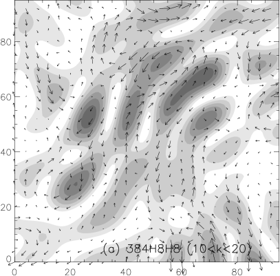
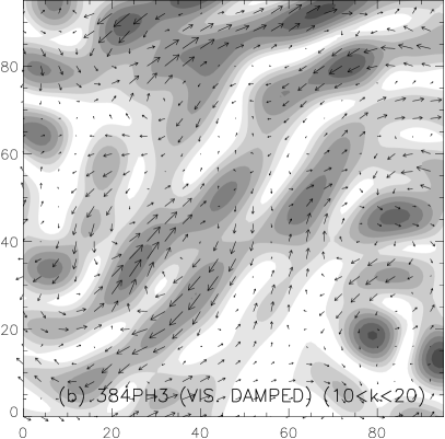
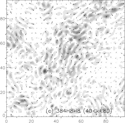
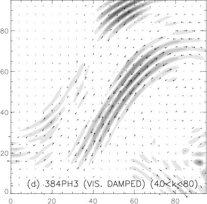
Figure 3: Magnetic structures in planes perpendicular to the mean magnetic field. (a) and (c): Ordinary MHD turbulence. The distribution of magnetic energy is more or less smooth. We do not observe scale-dependency. (b) and (d): Viscosity-damped MHD turbulence. In the Run 384PH3-B₀1, the viscosity-damped regime emerges below the dissipation scale at $k_{c}\sim 10$ (see Figure 1(b)). Panel (b) is not much different from panel (a) because the corresponding scale is not far from the dissipation scale. In panel (d), the distribution of magnetic energy is very intermittent. Panels (b) and (d) illustrate that intermittency is more pronounced at small scales.

Figure 4: Fractional volume (X-axis) vs. fractional magnetic energy in the volume (Y-axis) (a: left) Ordinary MHD strong turbulence: intermittency is independent of scale. (b: right) Viscosity-damped MHD turbulence: smaller scales show a higher concentration of magnetic energy.

5 High order statistics

Spectra do not provide a full description of turbulence. Another useful source of information is the scaling of high order structure functions. The p-th order (longitudinal) velocity structure function $SF_{p}$ and scaling exponents $\zeta(p)$ are defined as

$$SF_{p}({\bf r})\equiv\langle|\left[{\bf v}({\bf x}+{\bf r})-{\bf v}({\bf x})\right]\cdot{\bf\hat{r}}|^{p}\rangle\propto r^{\zeta(p)},$$ (15)

where the angle brackets denote averaging over x. In this section, we discuss the scaling of $\zeta(p)$ in ordinary and viscosity-damped turbulence.

5.1 Ordinary turbulence

The scaling relation suggested by She & Leveque (1994) contains three parameters (see Politano & Pouquet 1995; Müller & Biskamp 2000): $g$ is related to the scaling $v_{l}\sim l^{1/g}$, $x$ related to the energy cascade rate $t_{l}^{-1}\sim l^{-x}$, and C, the co-dimension of the dissipative structures:

$$\zeta(p)={p\over g}(1-x)+C\left(1-(1-x/C)^{p/g}\right).$$ (16)

For incompressible hydrodynamic turbulence, She & Leveque (1994) obtained

$$\zeta^{SL}(p)=p/9+2\left[1-(2/3)^{p/3}\right],$$ (17)

using $g=3$, $x=2/3$, and $C=2$, implying that dissipation happens over 1D structures (e.g. vortices).

In 3-dimensional MHD turbulence, there have been three recent developments for the scaling of the structure function exponents $\zeta(p)$. First, Müller & Biskamp (2000) extended the She-Leveque model to incompressible MHD turbulence and obtained

$$\zeta^{MB}(p)=p/9+1-(1/3)^{p/3},$$ (18)

where they used $g=3$, $x=2/3$, and assumed that the dissipating structures are 2-dimensional (i.e $C=3-2=1$). Their numerical calculations for decaying MHD turbulence without mean field show that scaling exponents for ${\bf z}^{\pm}\equiv{\bf v}\pm{\bf b}$ follow this relation very closely. Second, CLV02a studied MHD turbulence in a strongly magnetized medium and showed that turbulent motions (i.e. velocity) in planes perpendicular to the local mean field directions follow the original She-Leveque scaling (equation (17)). Physically this might mean that the dissipative structures are again 1D hydrodynamic-type vortices. However, more probably, this may just mean that the dissipation structures look like one-dimensional in the (perpendicular) slices of 3D MHD turbulence. Third, Boldyrev (2002) assumed that in compressible turbulence dissipation happens over 2D structures, i.e. $C=1$ and eq. (18) for $\zeta$. This scaling was supported by compressible MHD simulations (Padoan et al. 2003a). Padoan et al. (2003a) showed that the velocity field in highly super-sonic MHD turbulence follows the scaling given by eq. (18) scaling, while in subsonic MHD turbulence it follows the scaling in equation (17).

Combined together these results look puzzling. One can see easily that there are at least two apparent contradictions. First, Cho et al.’s (CLV02a) result conflicts with Müller & Biskamp’s result. This discrepancy could be attributed to the different simulation parameters. For example, CLV02a used a strong mean field while MB00 used no mean field. However, according to Müller & Biskamp (2003), the difference in $B_{0}$ does not resolve this problem. Second, Padoan et al. (2003a) is at odds with Müller & Biskamp (2000): Padoan et al.’s results for low Mach number do not converge to the incompressible case. The difference in $B_{0}$ looks marginal: Müller & Biskamp (2000) used a zero mean magnetic field while Padoan et al. (2003a) used a weak mean magnetic field.

These contradictions have led us to revisit the issue of intermittency in strong MHD turbulence. In Figure 5(a), we plot longitudinal velocity structure functions $SF_{p}$. The calculations are done in the perpendicular planes in the local frame of reference, where the parallel axis is aligned with the local mean magnetic field (see CLV02a):

$$SF_{p}^{local}({\bf r})\equiv\langle|\left[{\bf v}({\bf x}+{\bf r}_{\perp})-{\bf v}({\bf x})\right]\cdot{\bf\hat{r}}_{\perp}|^{p}\rangle,$$ (19)

where ${\bf r}_{\perp}$ is perpendicular to local mean field and ${\bf\hat{r}}_{\perp}$ is the unit vector parallel to ${\bf r}_{\perp}$. We show the second, third, fifth, and 10th order structure functions. We observe that the slopes are slightly shallower than those of She-Leveque model. Here the results are for longitudinal structure functions, which mostly reflect Alfven mode statistics in the perpendicular planes. However, when we use normal structure functions ($\langle|\left[{\bf v}({\bf x}+{\bf r}_{\perp})-{\bf v}({\bf x})\right]|^{p}\rangle$), which reflect both Alfven and pseudo-Alfven statistics, the $\zeta(p)$’s show a larger deviation from the She-Leveque model. This may be understood if the pseudo-Alfven modes have different scaling exponents. We can separate out the scaling of pseudo-Alfven modes when we use transverse structure functions in the perpendicular planes in local frame. We can also capture them using longitudinal structure functions in the parallel directions in local frame. However, we will not pursue this issue further here.

In Figure 5(b), we plot the normalized differential slope, $[d\ln SF_{p}/d\ln r]/[d\ln SF_{3}/d\ln r]$, for local frame velocity structure functions. In the actual calculations, we use $[d\ln SF_{p}/d\ln r](r)\approx\ln[SF_{p}(r+4)/SF_{p}(r-4)]/\ln[(r+4)/(r-4)]$. From the Figure, we obtain the $\zeta(p)$’s by averaging the differential slope over $r\in[20,45]$. In general, normalizing the differential slope using $SF_{3}$ gives better-defined scaling exponents, which was noted in Müller & Biskamp (2003) and by Boldyrev (private communication).

In Figure 5(c), we plot the $\zeta(p)$’s obtained this way for velocity, magnetic field, and $z^{\pm}$. The scaling exponents for velocity show reasonable agreement with the She-Leveque model, in agreement with CLV02a. Those for the magnetic field follow the Müller-Biskamp model for small $p$ but level off and do not change much when $p>7$. Those for Elsasser variables $z^{\pm}$ lie between those for the velocity and magnetic fields.

In Figure 5(d), we plot $\zeta(p)$’s calculated in the global frame, in which coordinate axes are aligned with the usual Cartesian axes. The method we used for Figure 5(d) is similar to the methods used by Müller & Biskamp (2000) and Padoan et al. (2003a), apart from the fact that our turbulence is strongly magnetized. It is worth noting that we get a good agreement with the Müller-Biskamp (2000) model for $z^{\pm}$ variables.

Our first result is that the scaling exponents obey the rule $\zeta^{magnetic}(p)<\zeta^{z}(p)<\zeta^{velocity}(p)$. It matters whether one uses Elsasser variables, velocity or magnetic field to determine the dimension of the dissipation structures. Our second result is that the dimension of the dissipation structures looks different when viewed in local and global frames of reference. It looks as if one dimensional vortices merge into two-dimensional sheets when viewed from the global system of reference. These differences should make us wary of a naive association of the corresponding parameters in eq.(16) with the dimensions of the dissipation structures in MHD turbulence.

This result can eliminate the contradiction between Müller & Biskamp (2000) and CLV02a: the former used the Elsasser variables in the global frame and the latter used velocity in the local frame for studying scaling exponents (see Figure 5(c) and (d)). Similarly, the conflict between Müller & Biskamp (2000) and Padoan et al. (2003a) can be partially relieved: the latter used velocity and, therefore, we expect that the scaling exponents in the latter are larger than those in the former. However, it is not certain from this that the discrepancy between the Padoan et al. (2003a) scalings at low Mach number and those in Müller & Biskamp (2000) in the incompressible case has been completely resolved. It is also unclear why the magnetic and velocity fields have different scalings. The sense of the difference suggests that the magnetic field is significantly more intermittent than the velocity field. Apparently this topic deserves further theoretical research.

(a)	(b)
(c)	(d)

Figure 5: The intermittency of ordinary turbulence (384H8H8-B₀1). (a: upper-left) Velocity structure functions (multiplied by arbitrary constants) in planes perpendicular to the local mean magnetic fields. (b: upper-right) Differential slopes normalized by that of the third-order structure function: $[d\ln SF_{p}/d\ln r]/[d\ln SF_{3}/d\ln r]$, where $SF_{p}$ is the p-th order longitudinal velocity structure function calculated in planes perpendicular to the local mean magnetic fields. The slope for $SF_{1}$ is the bottom curve and that for $SF_{12}$ is the top curve. (c: lower-left) Normalized structure function exponents in perpendicular directions in the local frame. The velocity exponents show a scaling similar to the She-Leveque model. The magnetic field shows a different scaling. (d: lower-right) Normalized structure function exponents in the global frame. Note that the result for $z^{\pm}$ is very similar to the Müller-Biskamp model.

5.2 High order structure functions in decaying compressible MHD turbulence

Above we speculated that there may not be a contradiction between the results by Müller & Biskamp (2000) and Padoan et al. (2003a). To test this we performed a numerical simulation for decaying compressible MHD turbulence without mean magnetic field. The compressible MHD code is described in detail in Cho & Lazarian (2002). We use the same numerical scheme described above. The initial kinetic and magnetic energy spectra are

$$E_{v}(k)\approx E_{b}(k)\approx k^{2}e^{-k^{2}/k_{0}^{2}},$$ (20)

where we take $k_{0}=2$. The initial phases of the individual Fourier components are random. The initial sonic Mach number (the ratio of the rms velocity to the sound speed) is $\sim 0.7$ and the density is constant.

Initially only small-$k$ Fourier components near $k=k_{0}$ are excited, but as the energy cascade begins to operate the large-$k$ Fourier components are excited. We measure high-order structure function statistics after the energy spectra develop inertial range (Figure 6(a)). Initially the velocity and magnetic fields have almost identical spectra (equation (20)). It is interesting that the magnetic energy spectrum is larger than its kinetic counterpart at later times (see Biskamp & Müller 2000 for a similar result in the incompressible case). Figure 6(b) shows the raw velocity structure functions. Figure 6(c) shows the normalized $\zeta(p)$ (i.e.$\zeta(p)/\zeta(3)$), which we obtain by averaging the slopes between $r=17$ and $r=34$. Interestingly, it appears that the velocity closely follows She-Leveque scaling while the magnetic field follows Müller-Biskamp scaling. The velocity scaling we find is indeed consistent with the result in Padoan et al. (2003a). However, since we do not resolve a sufficiently long inertial range (see the spectra), the results in Figure 6(c) should be regarded as very tentative. We will present a comprehensive study of higher order statistics elsewhere.

Figure 6: Compressible decaying MHD turbulence (COM2). The mean magnetic field is zero: B₀=0. (a: left) Spectra. (b: middle) Structure functions in the global frame. (c: right) Normalized scaling exponents $\zeta(p)$ in the global frame. The magnetic and velocity fields show different scalings.

5.3 Viscosity-damped turbulence

The run 384PH3-B₀1 has a very limited inertial range for the magnetic field, and is not suitable for the study of scaling exponents. We use the run 256PH8-B₀0.5 ($\nu=0.06$ and $\eta=hyper-diffusion$) instead. In this run, the mean field strength is reduced to 0.5 because the rms velocity is $\sim$0.4 due to strong viscous damping. The energy spectra is plotted in Figure 7. This run also clearly shows scale dependent intermittency. The parallel wavenumber $k_{\|}$ shows a very slow increase, a factor of $\sim 2$ from $k=5$ to $k=70$. Viscous damping occurs right at the energy injection scale (Figure 7(a)). The magnetic spectrum shows a slope roughly consistent with $-1$. Here we consider only the magnetic scaling exponents.

Figure 7(b) shows the structure functions for magnetic field. The calculation is done in perpendicular planes in local frame. Figure 7(c) shows that the scaling exponents becomes negative when $p$ is larger than 8.

In the original She-Leveque model, they first obtained the scaling relation for high order statistics of energy dissipation averaged over a ball of size $l$, $\epsilon_{l}$: $<\epsilon_{l}^{p}>\sim l^{\tau_{p}}$ with $\tau_{p}^{SL}=-2p/3+2[1-(2/3)^{p}]$. Then, using the Kolmogorov refined similarity hypothesis, $\epsilon_{l}\approx v_{l}^{3}/l$ or $v_{l}\approx l^{1/3}\epsilon_{l}^{1/3}$, they obtained

$$\zeta^{SL}(p)=p/3+\tau_{p/3}.$$ (21)

Note that $\tau_{p}<0$ and, hence, $\zeta^{SL}(p)<p/3$. In viscosity-damped MHD turbulence, we cannot use the Kolmogorov refined similarity hypothesis directly. Instead, from $\epsilon_{l}\approx b_{l}^{2}/l^{0}$ or $b_{l}\approx\epsilon^{1/2}$, we expect

$$\zeta^{damped}(p)=\tau_{p/2}.$$ (22)

As in She-Leveque (1994; see also Politano & Pouquet 1995), we may write

$$\tau_{p}=-xp+C[1-(1-x/C)^{p}],$$ (23)

where $x$ and $C$ are defined as in equation (16). When we substitute $x=0$, we get $\tau_{p}=0$ and $\zeta^{damped}(p)=0$. However, the 2-parameter She-Leveque model in equation (16) may not be applicable to the case of $x=0$.

Despite the evident problems with extending the She-Leveque model into the viscosity-damped regime, a crude estimate for the $\zeta(p)$ can be obtained from the theoretical model discussed in §2. Given the extreme intermittency of the magnetic field we expect that equation (15) will give

$$SF_{p}(l)\sim\hat{b}_{l}^{p}\phi_{l}\sim l^{1-p/2},$$ (24)

or

$$\zeta(p)=1-{p\over 2}.$$ (25)

However, the rise in magnetic field strength at small length scales introduces a competing contribution from the resistive scale, since for $p>2$ the rise in local magnetic field strength overwhelms the decrease in the filling factor as a function of scale. This small scale contribution is not a function of $l$ and when it dominates we expect $\zeta(p)\sim 0$. Putting all this together, we see that our simple model for the viscosity-damped regime predicts that $\zeta(1)$ will lie between $0$ and $0.5$, $\zeta(2)\sim 0$, and when $p>2$ we expect that $\zeta(p)$ will become negative and then asymptote to $0$ at large $p$.

Comparing this prediction to Figure (7) we see that this naive prediction enjoys some qualitative success, but is certainly not exactly correct. Part of the problem may lie in the limited resolution of our numerical simulation. For example, the expectation that the magnetic energy spectrum follows a $k^{-1}$ scaling is fairly compelling, but in that case we would expect $\zeta(2)=0$. The scaling in the simulation is slightly steeper (Figure 7(a)). The failure of the higher order exponents to match the theoretical model may be part of the same problem, but it is also likely to reflect the crude nature of the model. Kolmogorov turbulence theory gives a passable match to $\zeta(2)$, but fails noticeably at higher $p$, and our model for the viscosity-damped MHD regime is not particularly more sophisticated.

Figure 7: Viscous damped turbulence (256PH8-B₀0.5). (a: left) Spectra. (b: middle) Magnetic structure functions in the local frame. (Those calculated in the global frame show similar behaviors.) (c: right) Magnetic structure function exponents, $\zeta(p)$, in the local frame (not normalized). The observed scaling exponents are at least close to the expected asymptote $\zeta(p)=0$.

6 Testing and Discussion

6.1 Viscosity-damped turbulence with physical diffusion

How real are the structures that we observe in the new regime of MHD turbulence? Could they be a numerical artifact?

We have used a third or higher order hyper-diffusion term to minimize the effects of magnetic diffusion. However, in general, high order hyper-diffusion suffers from a bottle-neck effect, which is characterized by a flattening of the energy spectrum near the dissipation scale. Therefore it is necessary to check if the tail of the magnetic fluctuations is a real physical effect and not due to a bottle-neck. Here, we present a run with a physical magnetic diffusion term (Run 256PP-B₀1; $\nu=0.015$, $\eta=0.001$).

In Figure 8(a), we see that, compared with its kinetic counterpart, the magnetic spectrum has more power at $k>10$. Although we cannot say much about the spectrum of the magnetic fluctuations at scales smaller than the viscous cutoff ($k_{c}\sim 7$), the existence of the new regime is evident in Figure 8(a). A visual inspection of the magnetic structures in Figure 9(a) exhibit intermittent structures similar to those seen in the case of hyper-diffusion. We see that the bottle-neck effect is not responsible for intermittent magnetic structures at small scales.

Figure 8: Spectra of runs without hyper-diffusion. We use the same physical viscosity ($\nu=0.015$) for velocity. (a: left) From an incompressible run with a physical magnetic diffusion (256PP-B₀1). We use a small physical magnetic diffusion coefficient ($\eta=0.001$). The kinetic spectrum declines quickly due to the large viscosity. The magnetic spectrum shows structures at small scales (i.e. $k>10$). (b: right) From a compressible MHD run (COM1). We use numerical diffusion. The rms Mach number is $\sim$0.5. Due to the large viscosity ($\nu=0.015$), the kinetic spectrum drops quickly for $k\gtrsim 7$. The magnetic spectrum shows structures at small scales (i.e. $k>10$). Note that the shape of the density spectrum ($E_{\rho}$) is similar to the magnetic spectrum. Figure (b) is from Cho & Lazarian (2003a,b).

Further testing of the viscous damped regime was performed in Cho & Lazarian (2003a,b). There, using the compressible code mentioned earlier, we calculated not only velocity and magnetic field strength, but also density fluctuations that arise from MHD turbulence in the viscosity-damped regime. We present our results in Figure 8(b), side by side with a plot of the incompressible simulation results. The similarity between the two are vivid. It is also evident that the shallow spectrum of magnetic fluctuations results in a shallow spectrum of density fluctuations. Theoretically we expect the density spectrum to follow a $k^{-1}$ law. Unfortunately, our low resolution does not allow us to test this prediction at the moment.

Figure 9(c) shows that the density also has intermittent structures below the viscous cutoff. The density fluctuations may be (anti-)correlated with magnetic structures (see Figure 9(b)). However, we will postpone further discussion of this point until higher resolution runs become available.

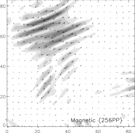
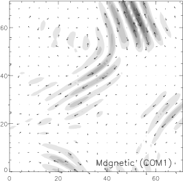
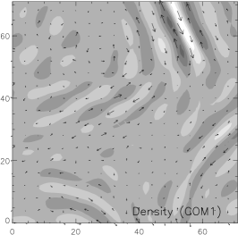
Figure 9: Intermittent small scale structures in a plane perpendicular to the mean magnetic field. (a: left) From an incompressible run with a physical magnetic diffusion (256PP-B₀1). Small scale ($k>20$) magnetic field structures show intermittency. (b: middle) From a compressible run (COM1). Small scale ($k>20$) magnetic field structures. (c: right) From COM1. Small scale ($k>20$) density structures.

6.2 Comparison with Observations

In this paper, we have considered properties of ordinary and viscosity-damped MHD turbulence. It is important to test our predictions with observations.

Indirect Evidence — Existence of density structures at scales smaller than a fraction of a parsec is particularly important for the small scale density structures in the ISM. We speculate that the power-law density tail might have some relation to the tiny-scale atomic structures (TSAS). Heiles (1997) introduced the term TSAS for the mysterious H I absorbing structures on the scale from thousands to tens of AU, discovered by Deiter, Welch & Romney (1976). Analogs are observed in NaI and CaII (Meyer & Blades 1996; Faison & Goss 2001; Andrews, Meyer & Lauroesch 2001) and in molecular gas (Marscher, Moore & Bania 1993). Recently Deshpande, Dwarakanath & Goss (2000) analyzed channel maps of opacity fluctuations toward Cas A and Cygnus A. They found that the amplitudes of density fluctuations at scales less than 0.1 pc are far larger than expected from extrapolation from larger scales, consistent with the existence of TSAS.

Measuring velocity and density spectra — Velocity channel analysis (VCA; Lazarian & Pogosyan 2000) is a recent technique that can extract velocity and density spectra. The technique predicts that the power spectra of spectral line intensity vary when the thickness of velocity channels changes. The compressible simulation in the previous subsection suggests that density may have a $k^{-1}$ spectrum below the viscous cutoff. At these scales, velocity effects should be suppressed. Deshpande et al. (2000) used absorption measurements to test the HI structure on subparsec scales and did not see the variations of the channel map spectra as they added their channels together. This meant that the velocity effects were negligible at the scales they studied. According to the VCA this meant that the shallow spectrum of density $k^{-\alpha}$ ($\alpha<1$) that they measured corresponds to real density fluctuations. This spectrum may arise from the new regime of MHD turbulence. Further tests, including those which use different techniques are necessary.

Information on the velocity statistics can also be obtained using centroids of velocity (see Munch 1958). Modified velocity centroids (MVCs) that are not sensitive to density fluctuations and can therefore be used for studies of velocity statistics were proposed in Lazarian & Esquivel (2003). They argued that combining the VCA and MVCs it is possible to get reliable measures of the underlying velocity spectra. It will be important to analyze the Deshpande et al. data using MVCs.

Studies of anisotropy — Testing scale-dependent anisotropy is a challenging problem, because scale-dependent anisotropy is averaged away when we observe turbulence from outside. The scale-dependent anisotropy is revealed only in a local frame of reference whose parallel axis is parallel to the local mean magnetic field (Cho & Vishniac 2000; CLV02a). Nevertheless, we can still study global anisotropy with 3D maps using velocity centroids (Lazarian, Pogosyan & Esquivel 2002) or 2D maps obtained from the Position-Position-Velocity data (Esquivel et al. 2003).

Higher order statistics — Scale-dependent intermittency is hard to study using observational data. Usually the noise increases rapidly as we go to higher order statistics. However, high order density structure function scalings have been used to study interstellar turbulence by Padoan et al. (2003b) and Padoan, Cambresy, & Langer (2003). Further studies of the problem are obviously required.

7 Summary

We have compared ordinary MHD turbulence and viscosity-damped MHD turbulence. They are different in many ways - in their spectra, in the degree of anisotropy and its scaling with length, and in the nature of intermittency in the turbulent cascade.

1. The spectra of ordinary strong MHD turbulence are compatible with Kolmogorov’s $k^{-5/3}$ spectrum. The magnetic spectra in viscosity-damped turbulence show a flatter spectrum: $E(k)\sim k^{-1}$.

2. Eddies in ordinary MHD turbulence show scale-dependent anisotropy consistent with the Goldreich & Sridhar model. Eddies in viscosity-damped MHD turbulence show extremely anisotropic structures - their parallel size does not decrease significantly with the perpendicular eddy size.

3. Intermittency of magnetic field strength in ordinary turbulence is not scale-dependent. Intermittency in viscosity-damped turbulence is scale-dependent: smaller scales are more intermittent.

4. The velocity and magnetic fields show different scaling exponents for high order structure functions.

5. Scaling exponents for the magnetic field in viscosity-damped MHD turbulence show very little change as order of the structure changes. They are generally small and change from positive at $p=1$ to negative values at moderate $p$.

Table 1: Simulations

Run	$N^{3}$	$\nu$	$\eta$	$B_{0}$	Note
384H8H8-$B_{0}$1	$384^{3}$	hyper	hyper ($\nabla^{16}$)	1	incompressible
384PH3-$B_{0}$1	$384^{3}$	.015	hyper ($\nabla^{6}$)	1	incompressible
256PH8-$B_{0}$0.5	$256^{3}$	.06	hyper ($\nabla^{16}$)	.5	incompressible
256PP-$B_{0}$1	$256^{3}$	.015	.001	1	incompressible
COM1	$216^{3}$	.015	numerical	1	compressible
COM2	$256^{3}$	numerical	numerical	0	compressible

References

- Andrews et al. (2001) Andrews, S. M., Meyer, D. M., & Lauroesch, J. T. 2001 ApJ, 552, L73
- Armstrong et al. (2001) Armstrong, J. W., Rickett, B. J., & Spangler, S. R. 1995, ApJ, 443, 209
- Biskamp & Müller (2000) Biskamp, D. & Müller, W.-C. 2000, Phys. of Plasmas, 7(12), 4889
- Boldyrev (2002) Boldyrev, S. 2002, ApJ, 569, 841
- Cho & Lazarian (2002a) Cho, J., Lazarian, A. 2002, Phy. Rev. Lett., 88, 245001
- Cho & Lazarian (2003a) Cho, J., Lazarian, A. 2003a, Rev. Mex. A.&A. (Serie de Conf.), 15, 293
- Cho & Lazarian (2003b) Cho, J., Lazarian, A. 2003b, MNRAS, submitted (astro-ph/0301062)
- Cho & Lazarian (2003c) Cho, J., Lazarian, A. 2003c, preprint (astro-ph/0301462)
- Cho et al. (2003) Cho, J., Lazarian, A., & Vishniac, E. 2003, in Turbulence and Magnetic Fields in Astrophysics, eds. E. Falgarone & T. Passot (Springer LNP), p56 (astro-ph/0205286)
- Cho et al. (2002a) Cho, J., Lazarian, A., & Vishniac, E. 2002a, ApJ, 564, 291 (CLV02a)
- Cho et al. (2002b) Cho, J., Lazarian, A., & Vishniac, E. 2002b, ApJ, 566, L49 (CLV02b)
- Cho & Vishniac (2000b) Cho, J. & Vishniac, E. 2000, ApJ, 539, 273
- Deshpande, Dwarakanath & Goss (2000) Deshpande, A. A., Dwarakanath, K. S., & Goss, W. M. 2000, ApJ, 543, 227
- Dieter, Welch & Romney (1976) Dieter,N. H., Welch, W. J., & Romney, J. D. 1976, ApJ, 206, L113
- Draine & Lazarian (1999) Draine, B. T. & Lazarian, A. 1999, ApJ, 512, 740
- Esquivel et al. (2003) Esquivel, A., Lazarian, A., Pogosyan, D., & Cho, J. 2003, MNRAS, accepted (astro-ph/0210159)
- Faison & Goss (2001) Faison, M. D. & Goss, W. M. 2001, AJ, 121, 2706
- Goldreich & Sridhar (1995) Goldreich, P. & Sridhar, S. 1995, ApJ, 438, 763
- Higdon (1984) Higdon, J. C. 1984, ApJ, 285, 109
- Heiles (1997) Heiles, C. 1997, ApJ, 481, 193
- Kolmogorov (1941) Kolmogorov, A. 1941, Dokl. Akad. Nauk SSSR, 31, 538
- Lazarian et al. (2002) Lazarian, A., Cho, J., & Yan, H. 2002, preprint (astro-ph/0211031)
- Lazarian & Esquivel (2003) Lazarian, A. & Esquivel, A. 2003, ApJL, submitted (astro-ph:0304007)
- Lazarian et al. (2003) Lazarian, A., Perosian, V., Yan, H., & Cho, J. 2003, in press (astro-ph/0301181)
- Lazarian & Pogosyan (2000) Lazarian, A. & Pogosyan, D. 2000, ApJ, 537, 720
- Lazarian et al. (2003) Lazarian, A., Pogosyan, D., & Esquivel, A. 2002, in Seeing Through the Dust, ASP Conf. Vol. 276, eds. A. Taylor, T. Landecker, & A. Willis (San Francisco), p. 182
- Lazarian et al. (2001) Lazarian, A., Pogosyan, D., Vázquez-Semadeni, E., & Pichardo, B. 2001, ApJ, 555, 130
- Lazarian & Vishniac (1999) Lazarian, A. & Vishniac, E. T. 1999, ApJ, 517, 700
- Lazarian et al. (2003) Lazarian, A., Vishnaic, E. T., & Cho, J. 2003, ApJ, submitted (LVC03)
- Lesieur (1990) Lesieur, M. 1990, Turbulence In Fluids (Dordrecht: Kluwer)
- Lithwick & Goldreich (2001) Lithwick, Y. & Goldreich, P. 2001, ApJ, 562, 279
- Maron & Goldreich (2001) Maron, J. & Goldreich, P. 2001, ApJ, 554, 1175
- Marscher et al. (1993) Marscher, A. P., Moore, E. M., & Bania, T. M. 1993, ApJ, 419, L101
- Matthaeus et al. (1998) Matthaeus, W. M., Oughton, S., Ghosh, S., Hossain, M. 1998 Phy. Rev. Lett., 81, 2056
- Meyer & Blades (1996) Meyer, D. M. & Blades, J. C. 1996, ApJ, 464, L179
- Müller & Biskamp (2000) Müller, W.-C. & Biskamp, D. 2000, Phys. Rev. Lett., 84(3), 475
- Müller & Biskamp (2003) Müller, W.-C. & Biskamp, D. 2003, in Turbulence and Magnetic Fields in Astrophysics, eds. E. Falgarone & T. Passot(Springer LNP), p3
- Munch (1958) Munch, G. 1958, Rev. Mod. Phys., 30, 1035
- Padoan et al. (2003) Padoan, P., Cambresy, L., & Langer, W. 2003, ApJ, 580, L57
- Padoan et al. (2003) Padoan, P., Jimenez, R., Nordlund, A., & Boldyrev, S. 2003a, preprint (astro-ph/0301026)
- Padoan et al. (2003b) Padoan, P., Boldyrev, S., Langer, W., & Nordlund, A. 2003b, ApJ, 583, 308
- Politano & Pouquet (1995) Politano, H. & Pouquet, A. 1995, Phy. Rev. E, 52, 636
- Schekochihin et al. (2002) Schekochihin, A., Maron, J., Cowley, S., & McWilliams, J. 2002, ApJ, 576, 806
- She & Leveque (1994) She, Z. & Leveque, E. 1994, Phy. Rev. Lett. 72, 336
- Shebalin et al. (1983) Shebalin, J. V., Matthaeus, W. H., & Montgomery, D. C. 1983, J. Plasma Phys., 29, 525
- Stanimirovic & Lazarian (2001) Stanimirovic, S. & Lazarian, A. 2001, ApJ, 551, L53
- Vazquez-Semadeni et al. (2000) Vazquez-Semadeni, E., Ostriker, E.C., Passot, T., Gammie, C.F., & Stone, J.M. 2000, in Protostars and Planets IV, eds. V. Mannings et al. (Tucson: University of Arisona Press), p.3
- Vestuto, Ostriker, & Stone (Vestuto et al.) Vestuto, J., Ostriker, E., & Stone, J. 2003, ApJ, in press (astro-ph/0303103)