Electron acceleration and heating in collisionless magnetic reconnection

Abstract

We discuss electron acceleration and heating during collisionless magnetic reconnection by using the results of implicit kinetic simulations of Harris current sheets. We consider and compare electron dynamics in plasmas with different $\beta$ values and perform simulations up to the physical mass ratio. We analyze the typical trajectory of electrons passing through the reconnection region, we study the electron velocity, focusing on the out-of-plane velocity, and we discuss the electron heating along the in-plane and out-of-plane directions.

I INTRODUCTION

Collisionless magnetic reconnection plays an important role in energetically active processes in plasmas Biskamp2000 ; Priest2000 . Magnetic reconnection takes place in plasmas characterized by different values of $\beta$. Theoretical, observational, and experimental results show that reconnection is present in the geomagnetic tail Oieoroset2001 , where local $\beta>>1$; in the Earth’s magnetopause Nishida1978 , where $\beta\approx 1$; in laboratory Syrovatsky1973 ; Gekelman1991 ; Yamada1999 ; Egedal2001 ; Furno2003 ; Taylor1996 , in the solar corona plasma Priest1982 , and in astrophysical plasmas, such as extragalactic jets Romanova1992 ; Blackman1996 ; Lesh1998 and flares in Active Galactic Nuclei (AGN) Lesch1997 , where $\beta\leq 1$.

During magnetic reconnection, magnetic energy is converted into kinetic and thermal energy of electrons and ions. In fact, electron heating and acceleration are signatures of magnetic reconnection. In the magnetotail, bursts of energetic electrons have been attributed to reconnection Terasawa1976 ; Baker1976 ; Baker1977 and there have been recent direct measurements of electron acceleration during magnetic reconnection Oieoroset2002 . Production of runaway electrons during sawtooth instabilities and disruptions is associated with magnetic reconnection in tokamaks Helander2002 . In solar flares, x-ray observations indicate that a large fraction of the total energy is released in accelerated electrons Lin1971 ; Lin1976 ; Gibson2002 . The observed synchroton radiation in extragalatic jets is thought to be generated by reacceleration or in-situ acceleration of electrons due to magnetic reconnection Romanova1992 ; Lesh1998 . It has been proposed that the detection of hard x-ray and $\gamma$-ray from AGN is due to the presence of electrons accelerated by magnetic reconnection Lesch1997 .

Electron dynamics in the reconnection region have been studied using analytical arguments Speiser1965 ; Zelenyi1990 ; Litvinenko1996 ; Litvinenko1997 , test particle theory Wagner1980 ; Sato1982 ; Scholer1987 ; Deeg1991 ; Vekstein1997 ; Birn2000 , self-consistent fluid simulations Nodes2003 , and kinetic simulations Loboeuf1982 ; Horiuchi1997 ; Hoshino2001 .

The aim of the present paper is to study the electron dynamics near the reconnection region with self-consistent kinetic simulations of high and low $\beta$ plasmas. The plasma $\beta$ is varied from very large ($\beta>>1$) to small ($\beta<1$) values and systems are simulated with an ion/electron mass ratio up to the physical value ($m_{i}/m_{e}=1836$). We consider two-dimensional reconnection in Harris current sheet configurations Harris1962 , triggered by an initial perturbation Birn2001 . We introduce a guide field to reduce the plasma $\beta$ and eliminate the null field region at the current sheet. To perform kinetic simulations, we use CELESTE3D Brackbill1985 ; Vu1992 ; Ricci2002a , an implicit Particle-in-Cell (PIC) code, which models both kinetic ions and electrons while allowing simulations with higher mass ratios.

We show that both the plasma $\beta$ and the mass ratio strongly affect the electron dynamics. In low-$\beta$ plasmas, the electron meandering orbits present in high $\beta$ plasmas disappear. We focus on the out-of-plane electron velocity, which remains localized in the high-$\beta$ case, and which is sizable also far from the reconnection region in low $\beta$ plasmas Horiuchi1997 . A strong influence of the mass ratio on the out-of-plane velocity is shown by the simulations and the relevant scaling law is deduced. We show that the heating process is non-isotropic in presence of a guide field; in particular, the particles are preferably heated in the out-of-plane direction. This anisotropy contributes to the break-up of the frozen-in condition for electrons and allows reconnection to happen.

The paper is organized as follows. Section II describes the physical system and the simulations. Section III presents the results of the simulations, focusing on the typical trajectory of the electrons that pass through the reconnection region and the evolution of the electron fluid velocity and temperature during reconnection.

II PHYSICAL SYSTEM

We consider a two-dimensional Harris current sheet in the $(x,z)$ plane Harris1962 , with an initial magnetic field given by

$$\mathbf{B}_{0}(z)=B_{0}\tanh(z/\lambda)\mathbf{e}_{x}+B_{y0}\mathbf{e}_{y}$$ (1)

and plasma particle distribution functions for the species $s$ ($s=e,i$) by

$$f_{0,s}(z,\mathbf{v}) = n_{0}\,\hbox{sech}^{2}(z/\lambda)\left(\frac{m_{s}}{2\pi k_{B}T_{s}}\right)^{3/2}\exp\left\{-\frac{m_{s}}{2k_{B}T_{s}}\left[v_{x}^{2}+(v_{y}-V_{s})^{2}+v_{z}^{2}\right]\right\}$$ (2)

$$+ n_{b}\left(\frac{m_{s}}{2\pi k_{B}T_{s}}\right)^{3/2}\exp\left(-\frac{m_{s}v^{2}}{2k_{B}T_{s}}\right)$$

We use the same physical parameters as the GEM challenge Birn2001 . The temperature ratio is $T_{i}/T_{e}=5$, the current sheet thickness is $\lambda=0.5d_{i}$, the background density is $n_{b}=0.2n_{0}$, and the ion drift velocity in the $y$ direction is $V_{i0}=1.67V_{A}$, where $V_{A}$ is the Alfvén velocity, and $V_{e0}/V_{i0}=-T_{e0}/T_{i0}$. The ion inertial length, $d_{i}=c/\omega_{pi}$, is defined using the density $n_{0}$. We apply periodic boundary conditions in the $x$ direction and perfect conductors in the $z$ direction.

The standard GEM challenge parameters model reconnection in high $\beta$ plasmas. To model low $\beta$ plasmas, it is possible to consider either a entirely different equilibrium Nishimura2003 , or one may introduce a guide field in the standard Harris sheet equilibrium. Herein, we follow the second approach and we introduce a guide field $B_{y}=B_{y0}$, with a spatially constant value at $t=0$. The simulations are performed with different mass ratios, ranging from $m_{i}/m_{e}=25$ (standard GEM mass ratio) to the physical mass ratio for hydrogen, $m_{i}/m_{e}=1836$. Following Birn et al. Birn2001 , the Harris equilibrium is modified by introducing an initial flux perturbation in the form

$$A_{y}=-A_{y0}\cos(2\pi x/L_{x})\cos(\pi z/L_{z})$$ (3)

with $A_{y0}=0.1B_{0}c/\omega_{pi}$, which puts the system in the non-linear regime from the beginning of the simulation.

The simulations shown in the present paper are performed using the implicit PIC code CELESTE3D, which solves the full set of Maxwell-Vlasov equations using the implicit moment method Brackbill1985 ; Vu1992 ; Ricci2002a . The implicit method allows more rapid simulations on ion length and time scales than are allowed with explicit methods, yet retains the kinetic effects of both electrons and ions. In particular, the explicit time step and grid spacing limits are replaced in implicit simulations by an accuracy condition, $v_{th,e}\Delta t<\Delta x$, whose principal effect is to determine how well energy is conserved. In the simulations shown below, we typically choose $\omega_{ce}\Delta t\approx 0.5$, $\Delta x/d_{i}=0.4$, and $\Delta z/d_{i}=0.2$.

Previous work on magnetic reconnection performed by CELESTE3D have proved that results from our implicit code match well the results of explicit codes Ricci2002a . Implicit simulations allow one to model physical mass ratios, with which it is possible to distinguish scaling laws associated with different break-up mechanisms Ricci2002b . CELESTE3D has also been employed in a comprehensive study of the physics of fast magnetic reconnection, in plasmas characterized by different $\beta$ values Ricci2003 .

III RESULTS

We have performed a set of simulations, using different mass ratios ($m_{i}/m_{e}=25,180,1836$) and introducing different guide fields: $B_{y0}=0$, with $\beta=\infty$ at the center of the current sheet; $B_{y0}=B_{0}$, with $\beta=1.2$; and $B_{y0}=5B_{0}$, with $\beta=0.048$. We note that a guide field changes drastically the magnetic configuration of the system as the X point is no longer a null-point, as it is in the $B_{y0}=0$ case.

The dynamics of magnetic reconnection in plasmas with different values of $\beta$ have been pointed out and summarized in a previous paper Ricci2003 . Figure 1 shows the reconnected flux, $\Delta\Psi$, defined as the flux difference between the X and the O points for all the simulations considered Ricci2003 . Even though an initial perturbation is applied, reconnection proceeds slowly during an initial transient phase (which lasts approximatively until $t\omega_{ci}\approx 10$), when the system adjust to the initial perturbation. Subsequently, reconnection develops rapidly until the saturation level is reached. Both the reconnection rate and the saturation level decrease when the guide field is increased. All the simulations show a similar evolution. The mechanism which breaks the electron frozen-in condition is provided by the off-diagonal terms of the electron pressure tensor for all the guide fields considered Ricci2003 ; Hesse2002 . The reconnection rate is enhanced by the whistler dynamics in high $\beta$ plasmas, and by the Kinetic Alfvén Waves dynamics in low $\beta$ plasmas Ricci2003 ; Biskamp1997a ; Sonnerup1979 ; Terasawa1983 ; Kleva1995 ; Rogers2001 , provided that $\beta>m_{e}/m_{i}$. When $\beta<m_{e}/m_{i}$, fast reconnection is not possible Biskamp1997b ; Ottaviani1993 .

Theoretical results and kinetic simulations Ricci2002b ; Kuznetsova2000 show that with $B_{y0}=0$, electrons flow towards the X point along the $z$ direction, where they are demagnetized in a region corresponding to the meandering length, $d_{ze}$. There they are accelerated by the reconnection electric field, $E_{y}$, in the $y$ direction. The electrons are then diverted by the $B_{z}$ field, gaining an outflow velocity in the $x$ direction, and becoming remagnetized at the meandering length, $d_{xe}$. The meandering lengths are defined as Ricci2002b ; Kuznetsova2000

$$d_{xe}=\left[\frac{m_{e}T_{e}}{e^{2}(\partial B_{z}/\partial x)^{2}}\right]^{1/4},d_{ze}=\left[\frac{m_{e}T_{e}}{e^{2}(\partial B_{x}/\partial z)^{2}}\right]^{1/4}$$ (4)

while the maximum inflow and outflow velocities scale as Ricci2002b ; Kuznetsova2000

$$v_{xe}=\left[\frac{e^{2}E^{4}_{y}}{4m_{e}T_{e}(\partial B_{z}/\partial x)^{2}}\right]^{1/4},v_{ze}=\left[\frac{e^{2}E^{4}_{y}}{4m_{e}T_{e}(\partial B_{x}/\partial z)^{2}}\right]^{1/4}$$ (5)

In the reconnection region, the electrons are unmagnetized and follow complex meandering orbits, which result in a non-gyrotropic electron distribution function and in off-diagonal terms of the electron pressure Hoshino1998 .

When a guide field is introduced, the meandering orbits disappear. Analytical estimates of the guide field at which this happens are given by Litvinenko1996 ; Litvinenko1997 . Nevertheless, the diagonal components of the electron pressure tensor are unequal, which contributes to the presence of off-diagonal pressure terms Ricci2003 ; Hesse2002 . These terms still constitute the break-up mechanism of the frozen-in condition Ricci2003 ; Hesse2002 . In the reconnection region, the electrons flow across the field line in the $(x,z)$ plane, while performing a Larmor motion around the out-of-plane magnetic field. Far from the reconnection region, the guide field causes additional components of the $\mathbf{E}\times\mathbf{B}$ force, which modify the ion and electron motion and cause asymmetric plasma flow.

Below, we describe in detail the typical trajectory of an electron passing through the reconnection region in high and low $\beta$ plasmas. Then, we focus on the electron fluid velocity, in particular on the out-of-plane velocity. Finally, we consider the electron distribution functions to evaluate the electron temperature.

III.1 Electron trajectory

Figure 2 shows a typical trajectory of an electron passing through the reconnection region in the case $B_{y0}=0$, and Fig. 3 shows the history of its velocity and kinetic energy.

In Fig. 2, the initial position of the particle is denoted by a plus sign, and its position at selected time steps by circles. ’X’ marks the position of the X point. Note that periodic boundary conditions are applied in the $x$ direction, as the behavior of the trajectory shows (the particle exits from the left and re-enters from the right). At the beginning, the electron is tied to a magnetic field line (magnetic field lines run mainly along the $x$ direction). Near the reconnection point, the electron decouples from the magnetic field and moves along the $z$ direction, reaching the X point at $t\omega_{ci}\approx 15$. The particle trajectory is meandering in the unmagnetized region. The outflow from the reconnection region takes place as soon as the electron reaches a region with stronger magnetic field. Then, the electron couples again to a magnetic line surrounding the O point, and starts again its gyration orbit around it.

In Fig. 3, all components of the particle velocity and the kinetic energy are plotted as a function of time. Initially, the electron is flowing along the $x$ direction, with a Larmor motion mostly in the $(y,z)$ plane, which is responsible for the high frequency oscillations of the velocity (the magnetic field line is mostly directed along $x$). During this phase, the electron kinetic energy is almost conserved. When the electron decouples from the magnetic field line as it crosses the reconnection region, it is accelerated by the reconnection electric field in the $y$ direction. This acceleration transfers magnetic field energy to electrons during magnetic reconnection. As Fig. 3 shows, while the electron is unmagnetized, the kinetic energy of the electron increases remarkably, showing high frequency oscillations due to the acceleration and de-acceleration by the electric field. When the electron leaves the reconnection region and again couples to the magnetic field, motion in $y$ becomes Larmor motion with a bigger radius, and the velocity directed along $y$ gained in the reconnection region is lost. The particle couples to a magnetic field line that surrounds the O point and starts to flow along it.

In Fig. 4 the electron trajectory is traced for a low $\beta$ plasma, with a strong guide field, $B_{y0}=5B_{0}$. Initially, the particle flows along the magnetic line, which is mainly directed along the $y$ direction, and executes a Larmor motion mostly in the $(x,z)$ plane. The particle then accelerates towards the X point, crosses magnetic lines in the $(x,z)$ plane, and gains an out-of-plane velocity which increases its kinetic energy (see Fig. 5). The particle still couples to the magnetic field and executes a Larmor orbit around the guide field. Meandering orbits are not present. In contrast to the case with $B_{y0}=0$, the electron maintains its $y$ velocity even when far from the reconnection region because now the gyration is in the $(x,z)$ plane around the $y$-directed guide field. Finally, the electron drifts along a magnetic field line around the O point maintaining a still significant $y$ velocity which decreases slowly because of the interactions of the electron with the non-drifting plasma background.

The presence of the guide field changes the nature of electron acceleration: without guide field, the $y$ velocity is lost while in presence of guide field is retained even far from the reconnection region Horiuchi1997 .

III.2 Electron fluid velocity

When $B_{y0}=0$, both kinetic simulations and theoretical results Ricci2002b ; Kuznetsova2000 show that the electrons are demagnetized at the electron meandering distance [see Eqs. (4)] and have an inflow and outflow velocity given by Eqs. (5). The scaling laws of the dimensions of the reconnection region and of the inflow and outflow velocity, based on the electron pressure as a break-up mechanism as derived in Ref. Kuznetsova2000 , have been verified up to the physical mass ratio Ricci2002b . In the presence of a guide field, new components of the $\mathbf{E}\times\mathbf{B}$ field arise, and the electron in-plane motion has been described in Refs. Ricci2003 ; Yin2003 .

Here, we focus on the electron out-of-plane velocity. In Fig. 6, the velocity along the axis $z=0$ is depicted with $B_{y0}=0$ for three different mass ratios, $m_{i}/m_{e}=25,180,1836$. The maximum out-of-plane velocity increases with the mass ratio. We note that the out-of-plane velocity is sizeable only in the reconnection region.

The out-of-plane velocity can be estimated for $B_{y0}=0$. The electron lifetime in the reconnection region, $\tau$, from Eqs. (4-5) is approximately

$$\tau\approx d_{xe}/v_{xe}+d_{ze}/v_{ze}\propto\left(\frac{m_{e}^{2}T_{e}^{2}}{e^{4}E_{y}^{4}}\right)^{1/4}$$ (6)

As the magnetic field is negligible in the reconnection region, the electrons are freely accelerated and the out-of-plane velocity can be estimated as

$$v_{y}\approx\frac{e}{m_{e}}E_{y}\tau$$ (7)

and, using Eq. (6), it follows that

$$v_{y}\propto v_{th,e}$$ (8)

Since the temperature of the electrons is the same for all mass ratios, it follows that the electron out-of-plane velocity scales with $1/\sqrt{m_{e}}$. The results presented in Fig. 6 fit well this scaling law, as is shown in Table I.

Figures 7 and 8 consider the effect of the guide field on the out-of-plane electron velocity. As the guide field allows the particles to flow more easily in the out-of-plane direction, the peak velocity increases remarkably when the guide field becomes stronger, Fig. 7. Moreover, the presence of the guide field changes the general pattern of the out-of-plane velocity, as shown in Fig. 8. When $B_{y0}=0$, the out-of-plane velocity is sizeable only near the reconnection region, where the electrons are accelerated by the electric field. The out-of-plane velocity is lost when the electrons become again magnetized and are diverted by the $B_{z}$ field. In presence of the guide field, the electrons maintain their $y$ velocity when they leave the reconnection region and orbit around the O point. Note that this conclusion is further supported by the analysis of particle orbits performed in the subsection above (III.b).

As a final remark, we note that the out-of-plane velocity evolves during magnetic reconnection, as is shown in Fig. 9. For all the guide fields considered, the electron velocity increases while reconnection proceeds (the evolution of the reconnected flux in these simulations is presented in Fig. 1). After reconnection saturates, the reconnection electric field vanishes and the electrons are no longer accelerated. The out-of-plane velocity in the former reconnection region decreases abruptly.

III.3 Electron temperature

The evolution of the electron temperatures in the reconnection region, $T_{xe}$, $T_{ye}$, and $T_{ze}$, are plotted in Fig. 10 for the three different guide field strengths. We note that $T_{xe}$, $T_{ye}$, and $T_{ze}$ are defined as the second moment of the distribution functions of the $x$, $y$, and $z$ velocity Cercignani1988 .

In the zero guide field case, the $T_{xe}$ and $T_{ye}$ evolution is similar (see Fig. 10a). $T_{xe}$ increases because the positive and negative outflow velocity causes an increases spread in the $x$ velocity. The heating in the $y$ direction is due to the electric field which, besides accelerating the electrons, spreads out their velocity, reflecting the variation in electron residence time in the reconnection region, which depends on their in-plane inflow and outflow velocity, and thus are accelerated by different amounts. After reconnection saturates, the heating process stops and electrons tend to thermalize, causing an increase in $T_{ze}$. We note that the total energy of the system is conserved during the simulation within an error of the order of 4% Ricci2003 .

When the guide field is introduced, both $T_{xe}$ and $T_{ze}$ remain almost constant at the initial level during the reconnection process, while $T_{ye}$ increases remarkably. The guide field introduces an higher electron mobility in the $y$ direction. Thus, the electron can be accelerated by the electric field more than in the $B_{y0}=0$ case along the $y$ direction, and the $y$ velocities spread out more, while $T_{ye}$ increases.

The anisotropy in the electron temperature contributes to the break-up of the frozen-in condition. In fact, in the presence of a guide field, the difference between the diagonal terms of the electron pressure tensor contributes to the off-diagonal terms, which are responsible for the break-up of the frozen-in condition Ricci2003 ; Hesse2002 , as it is Hesse2002

$$P_{xye}=-\frac{P_{zze}}{\omega_{ce}}\frac{\partial v_{ye}}{\partial z}+\frac{B_{x}}{B_{y}}(P_{yye}-P_{zze})$$ (9)

$$P_{yze}=-\frac{P_{xxe}}{\omega_{ce}}\frac{\partial v_{ye}}{\partial x}+\frac{B_{z}}{B_{y}}(P_{yye}-P_{xxe})$$ (10)

Since $P_{yye}-P_{zze}=n_{e}(T_{ye}-T_{ze})$ and $P_{yye}-P_{zze}=n_{e}(T_{ye}-T_{ze})$, the importance of the anisotropy in the electron temperature is evident.

IV CONCLUSIONS

In the present paper, the electron dynamics during magnetic reconnection has been studied by showing and discussing results of kinetic simulations of Harris current sheets. Simulations with different plasma $\beta$ and different mass ratio have been considered.

By varying the guide field, we have been able to model reconnection in systems such as the magnetotail ($B_{y0}=0$), the magnetopause ($B_{y0}=B_{0}$), laboratory and astrophysical plasmas ($B_{y0}=5B_{0}$).

By studying the typical electron trajectories, we have shown that, when the plasma $\beta$ is decreased, the electrons mainly perform Larmor motion around the guide field even in the reconnection region, and that meandering orbits disappear. In all the cases, electrons are accelerated by the reconnection electric field along the $y$ direction and their velocity increases with the guide field. Moreover, the out-of-plane velocity increases during reconnection. In high $\beta$ plasmas, the out-of-plane velocity is sizable only in the electron reconnection region. With a guide field, the out-of-plane velocity is globally relevant. The mass ratio has a strong influence on the out-of-plane velocity and the scaling law of interest is derived. The study of the electron temperature in the reconnection region has shown a strong heating anisotropy in presence of a guide field, which contributes to the break-up of the electron frozen-in condition.

In closing, we note that we plan to develop the present work in two directions. First, we plan to introduce the relativistic equations of motion in CELESTE3D, in order to represent better the electron physics when relativistic effects become important. Second, an experimental setup has been built at the Los Alamos National Laboratory to study reconnection experimentally in plasmas with different $\beta$ Furno2003 . We plan to compare our simulation results with the experiments.

• Fig. 1 (from Ref. Ricci2003 ): Reconnected flux (normalized to $B_{0}c/\omega_{pi}$), for $m_{i}/m_{e}=25$ (a), $m_{i}/m_{e}=180$ (b), and $m_{i}/m_{e}=1836$ (c), and $B_{y0}=0$ (solid line), $B_{y0}=B_{0}$ (dashed line), $B_{y0}=5B_{0}$ (dotted line).

• Fig. 2: Electron trajectory in the $(x,z)$ plane, for $B_{y0}=0$ and $m_{i}/m_{e}=25$. The position of the particle at different times is marked by circles, the starting position by a plus sign. The position of the X point is denoted by the x-mark. Note the periodic boundary conditions in the $x$ direction.

• Fig. 3: Velocities $v_{x}$ (a), $v_{y}$ (b), $v_{z}$ (c) and kinetic energy (d), as a function of time, for the electron whose trajectory is represented in Fig. 2.

• Fig. 4: Electron trajectory in the $(x,z)$ plane, for $B_{y0}=5B_{0}$ and $m_{i}/m_{e}=25$. The position of the particle at different times is marked by circles, the starting position by a plus sign. The position of the X point is denoted by the x-mark. Note the periodic boundary conditions in the $x$ direction.

• Fig. 5: Velocities $v_{x}$ (a), $v_{y}$ (b), $v_{z}$ (c) and kinetic energy (d), as a function of time, for the electron whose trajectory is represented in Fig. 4.

• Fig. 6: Electron out-of-plane velocity at $z=0$, when $\Delta\Psi\approx 1$, for the simulations with $B_{y0}=0$ and $m_{i}/m_{e}=25$ (dashed line), $m_{i}/m_{e}=180$ (dotted line), and $m_{i}/m_{e}=1836$ (solid line).

• Fig. 7: Electron out-of-plane velocity at $z=0$, when $\Delta\Psi\approx 1$, for the simulations with $B_{y0}=B_{0}$ (a) and $B_{y0}=5B_{0}$ (b), $m_{i}/m_{e}=25$ (dashed line), $m_{i}/m_{e}=180$ (dotted line), and $m_{i}/m_{e}=1836$ (solid line).

• Fig. 8: Electron out-of-plane velocity when $\Delta\Psi\approx 1$, for the simulations with $B_{y0}=B_{0}$ (a) and $B_{y0}=5B_{0}$ (b), for the simulations with $m_{i}/m_{e}=180$.

• Fig. 9: Evolution of the average out-of-plane electron velocity, $v_{y}$ in the reconnection region, for the simulation with $m_{i}/m_{e}=25$, and guide field $B_{y0}=0$ (a), $B_{y0}=B_{0}$ (b), and $B_{y0}=5B_{0}$ (c).

• Fig. 10: Evolution of the electron thermal velocity $v_{thx,e}$ (solid), $v_{thy,e}$ (dashed), and $v_{thz,e}$ (dotted), in the reconnection region for the simulation with $m_{i}/m_{e}=25$ and $B_{y0}=0$ (a) and $B_{y0}=5B_{0}$ (b).

Table I.Comparison between the simulation results and the scaling law in Eq. (8)

Ratio	Simulation result	Scaling law
$\frac{v_{y}(m_{i}/m_{e}=180)}{v_{y}(m_{i}/m_{e}=25)}$	2.9	2.7
$\frac{v_{y}(m_{i}/m_{e}=1836}{v_{y}(m_{i}/m_{e}=25)}$	7.0	8.6

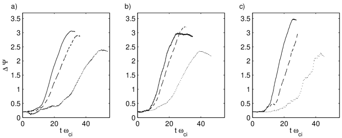
Figure 1:

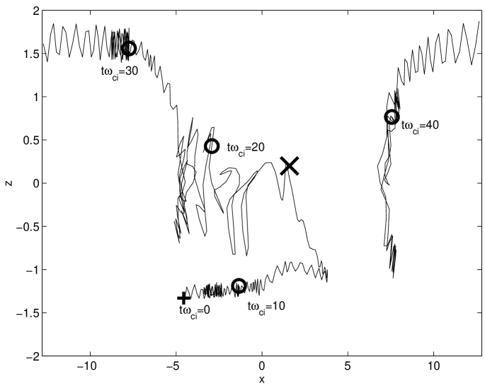
Figure 2:

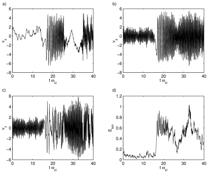
Figure 3:

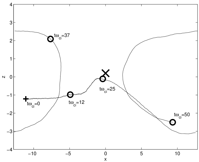
Figure 4:

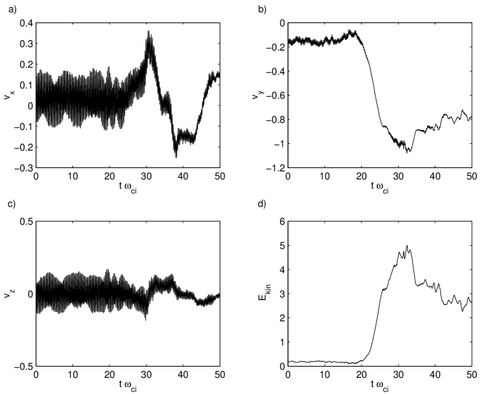
Figure 5:

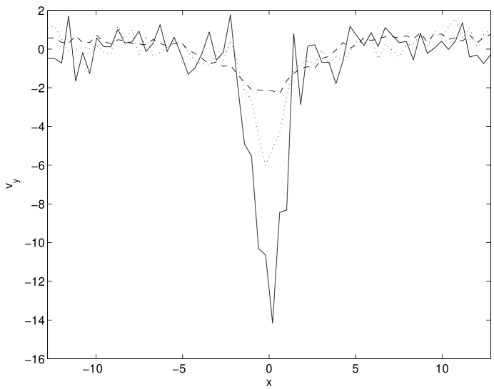
Figure 6:

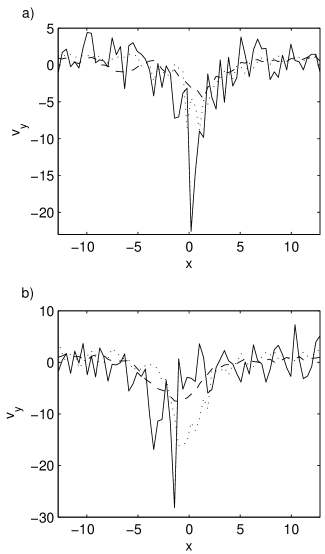
Figure 7:

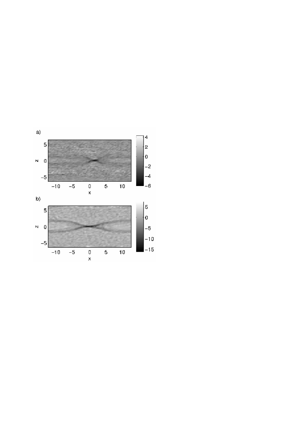
Figure 8:

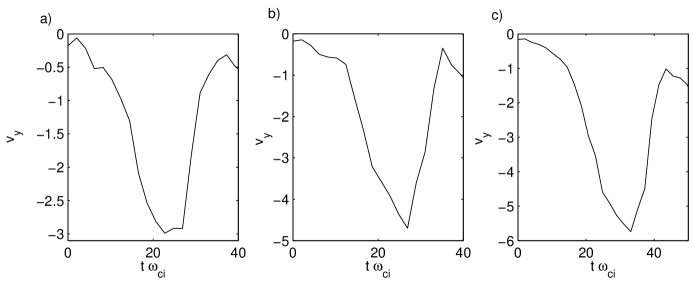
Figure 9:

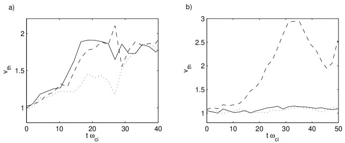
Figure 10:

References

- (1) D. Biskamp, Magnetic Reconnection in Plasmas (Cambridge University Press, Cambridge, 2000).
- (2) E.R. Priest and T. Forbes Magnetic Reconnection: MHD Theory and Applications (Cambridge University Press, New York, 2000).
- (3) M. Øieroset, T.D. Phan, M. Fujimoto, R.P. Lin, and R.P. Lepping, Nature 412, 414 (2001).
- (4) Nishida A., Geomagnetic Diagnostics of the Magnetosphere (Springer-Verlag, New York, 1978).
- (5) S. I. Syrovatsky, Sov. Phys. Tech. Phys. 18, 580 (1973).
- (6) W. Gekelman, H. Pfister, Z. Lucky, J. Bamber, D. Leneman, and J. Maggs, Rev. Sci. Instrum. 62, 2875 (1991).
- (7) M. Yamada, J. Geophys. Res. 104, 14529 (1999).
- (8) J. Egedal, A. Fasoli, D. Tarkowski, and A. Scarabosio, Phys. Plasmas 8, 1935 (2001).
- (9) I. Furno, T. Intrator, E. Torbert, C. Carey, M. D. Cash, J. K. Campbell, W. J. Fienup, C. A. Werley, G. A. Wurden, and G. Fiksel, Rev. Sci. Instrum. 74, 2324 (2003).
- (10) J.B. Taylor, Rev. Mod. Phys. 28, 243 (1986).
- (11) Priest, E.R., Solar Magnetohydrodynamics, (Reidel, Dordrecht, 1982).
- (12) M.M. Romanova, and R.V.E. Lovelace, Astron. Astrophys. 262, 26 (1992).
- (13) E. G. Blackman, Astrophys. J. Lett. 456, LT87 (1996).
- (14) H. Lesch and G.T. Birk, Astrophys. J. 499, 167 (1998).
- (15) H. Lesch and G.T. Birk, Astron. Astrophys. 324, 461 (1997).
- (16) T. Terasawa and A. Nishida, Planet. Space Sci. 24, 855 (1976).
- (17) D.N. Baker and E.C. Stone, Geophys. Res. Lett. 3, 557 (1976).
- (18) D.M. Baker and E.C. Stone, J. Geophys. Res. 82, 1532 (1977).
- (19) M. Øieroset, R.P. Lin, T.D. Phan,, D.E. Larson, and S.D. Bale, Phys. Rev. Lett. 89, 195001 (2002).
- (20) P. Helander, L.-G. Eriksson, and F. Andersson, Plasma Phys. Control. Fusion 44, B247 (2002).
- (21) R.P. Lin and H.S. Hudson, Sol. Phys. 17, 412 (1971).
- (22) R.P. Lin and H.S. Hudson, Sol. Phys. 50, 153 (1976).
- (23) S.E. Gibson et al., Astrophys. J. 574, 1021 (2002).
- (24) T.W. Speiser, J. Geophys. Res. 70, 4291 (1965).
- (25) L.M. Zelenyi, J.G. Lominadze, and A.L. Taktakishvili, J. Geophys. Res. 95, 3883 (1990).
- (26) Y.E. Litvinenko, Astrophys. J. 462, 997 (1996).
- (27) Y.E. Litvinenko, Phys. Plasmas 4, 3439 (1997).
- (28) J.S. Wagner, P.C. Gray, J.R. Kan, and S.-I. Akasofu, Planet. Space Sci. 4, 391 (1981).
- (29) T. Sato, T. Matsumoto, and K. Nagai, J. Geophys. Res. 87, 6089 (1982).
- (30) M. Scholer and F. Jamitzky, J. Geophys. Res. 92, 12181 (1987).
- (31) H.-J. Deeg, J.E. Borovsky, and N. Duric, Phys. Fluids B 9, 2660 (1991).
- (32) G.E. Vekstein, and P.K. Browning, Phys. Plasmas 4, 2261 (1997).
- (33) J. Birn, M.F. Thomsen, JE. Borovsky, G.D. Reeves, and M. Hesse, Phys. Plasmas 7, 2149 (2000).
- (34) C. Nodes, G.T. Birk, H. Lesch, and R. Schopper, Phys. Plasmas 10, 835 (2003).
- (35) J.N. Leboeuf, T. Tajima, J.M. Dawson, Phys. Fluids 25, 784 (1982).
- (36) R. Horiuchi and T. Sato, Phys. Plasmas 4, 277 (1997).
- (37) M. Hoshino, T. Mukai, T. Terasawa, and I. Shinohara, J. Geophys. Res. 106, 25979 (2001).
- (38) E.G. Harris, Nuovo Cimento Soc. Ital. Fis. A-D 23, 115 (1962).
- (39) J. Birn et al., J. Geophys. Res. 106, 3715 (2001).
- (40) J.U. Brackbill and D.W. Forslund, Simulation of low frequency, electromagnetic phenomena in plasmas, in Multiple tims Scales, J.U. Brackbill and B.I. Cohen Eds., (Accademic Press, Orlando, 1985), pp. 271-310.
- (41) H.X. Vu and J.U. Brackbill, Comput. Phys. Commun. 69, 253 (1992).
- (42) P. Ricci, G. Lapenta, and J.U. Brackbill, J. Comp. Phys. 183, 117 (2002).
- (43) K. Nishimura, S.P. Gary, H. Li, and S.A. Colgate, Phys. Plasmas 10, 347 (2003).
- (44) P. Ricci, G. Lapenta, and J.U. Brackbill, Geophys. Res. Lett. 29(23), 2008, 10.1029/2002GL015314 (2002).
- (45) P. Ricci, G. Lapenta, J.U. Brackbill, Kinetic simulations of collisionless magnetic reconnection in presence of a guide field, (J. Geophys. Res., submitted).
- (46) M. Hesse, M. Kuznetsova, and M. Hoshino, Geophys. Res. Lett. 29, 2001GL014714 (2002).
- (47) D. Biskamp, Phys. Plasmas 4, 1964 (1997).
- (48) B.U.O. Sonnerup, Magnetic Field Reconnection, in Solar System Plasma Physics, vol. III, edited by L.T. Lanzerotti, C.F. Kennel, and E.N. Parker, p. 45, North-Holland, New York, 1979.
- (49) Terasawa, T., Geophys. Res. Lett. 10, 475 (1983).
- (50) Kleva, R.G., J.F. Drake, and F.L. Waelbroeck, Phys. Plasmas 2, 23 (1995).
- (51) B.N. Rogers, R.E. Denton, J.F. Drake, and M.A. Shay, Phys. Rev. Lett. 87, 195004 (2001).
- (52) Biskamp, D., E. Schwarz, J.F. Drake, Phys. Plasmas 4, 1002 (1997).
- (53) M. Ottaviani and F. Porcelli, Phys. Rev. Lett. 71, 3802 (1993).
- (54) M.M. Kuznetsova, M. Hesse, and D. Winske, J. Geophys. Res. 105, 7601 (2000).
- (55) M. Hoshino, Kinetic Ion behavior in Magnetic Reconnection Region, in A. Nishida, D.N. Baker, and S.W.H. Cowley, New Perspectives on the Earth’s Magnetotail, Geophys. Mono., Vol. 105, pp. 153-166 , Amer. Geophys. Union, Washington D.C.
- (56) L. Yin and D. Winske, Plasma pressure tensor effects on reconnection: hybrid and Hall-magnetohydrodynamics simulations, Phys. Plasmas 10, 1595 (2003).
- (57) C. Cercignani, The Boltzmann equation and its applications (Springer-Verlag, New York, 1988).
-
•