Cosmological Variation of the Fine Structure Constant from an Ultra-Light Scalar Field: The Effects of Mass

Abstract

Cosmological variation of the fine structure constant $\alpha$ due to the evolution of a spatially homogeneous ultra-light scalar field ($m\sim H_{0}$) during the matter and $\Lambda$ dominated eras is analyzed. Agreement of $\Delta\alpha/\alpha$ with the value suggested by recent observations of quasar absorption lines is obtained by adjusting a single parameter, the coupling of the scalar field to matter.

Asymptotically $\alpha(t)$ in this model goes to a constant value $\overline{\alpha}\approx\alpha_{0}$ in the early radiation and the late $\Lambda$ dominated eras. The coupling of the scalar field to (nonrelativistic) matter drives $\alpha$ slightly away from $\overline{\alpha}$ in the epochs when the density of matter is important.

Simultaneous agreement with the more restrictive bounds on the variation $|\Delta\alpha/\alpha|$ from the Oklo natural fission reactor and from meteorite samples can be achieved if the mass of the scalar field is on the order of 0.5–0.6 $H_{\Lambda}$, where $H_{\Lambda}=\Omega_{\Lambda}^{1/2}H_{0}$.

Depending on the scalar field mass, $\alpha$ may be slightly smaller or larger than $\alpha_{0}$ at the times of big bang nucleosynthesis, the emission of the cosmic microwave background, the formation of early solar system meteorites, and the Oklo reactor. The effects on the evolution of $\alpha$ due to nonzero mass for the scalar field are emphasized.

An order of magnitude improvement in the laboratory technique could lead to a detection of $(\dot{\alpha}/\alpha)_{0}$.

1 Introduction

Recent observations by Webb et al. [1, 2] of absorption lines in quasar spectra provide evidence for a variation of the fine structure constant

$$\frac{\Delta\alpha}{\alpha}=\frac{\alpha(t)-\alpha_{0}}{\alpha_{0}}=(-0.57\pm 0.10)\times 10^{-5}$$ (1)

averaged over the redshift range $0.2\leq z\leq 3.7$ (“$\alpha$ was smaller in the past”), where $\alpha_{0}$ is the present-day value of the fine structure constant. This type of variation of $\alpha$, as well as variation of other dimensionless coupling constants, is predicted by theories which unify gravity and the standard model forces. For example, string and supergravity theories predict the existence of massless or ultra-light scalar fields (dilaton or moduli fields) which through their dynamical evolution can cause temporal variation of coupling constants.

This investigation will consider cosmological variation of the fine structure constant due to the evolution of a spatially homogeneous ultra-light scalar field ($m\sim H_{0}$, where $H_{0}$ is the present value of the Hubble parameter) during the matter and $\Lambda$ dominated eras. We will assume a flat Friedmann-Robertson-Walker universe, with $\rho_{c0}=\rho_{m0}+\rho_{r0}+\rho_{\Lambda}\approx\rho_{m0}+\rho_{\Lambda}$ today, where $\rho_{c0}$ is the present value of the critical density for a flat universe, and $\rho_{m0}$, $\rho_{r0}\ll\rho_{m0}$ , and $\rho_{\Lambda}$ are the present energy densities in (nonrelativistic) matter, radiation, and the cosmological constant respectively. Ratios of present energy densities to the present critical density are denoted by $\Omega_{m}=\rho_{m0}/\rho_{c0}$, $\Omega_{r}=\rho_{r0}/\rho_{c0}$, and $\Omega_{\Lambda}=\rho_{\Lambda}/\rho_{c0}$.

The scalar field $\phi$ may provide the cosmological constant energy density at the minimum of its potential $V(\overline{\phi})$. In the model presented here, the energy density $\rho_{\phi}-V(\overline{\phi})$ of the scalar field is always very small compared with the critical energy density in the radiation, matter, and $\Lambda$ (dominated) eras, so that the standard Friedmann-Robertson-Walker evolution of the universe is not affected by displacements of $\phi$ from $\overline{\phi}$.

Agreement of $\Delta\alpha/\alpha$ with the quasar data can be obtained by adjusting a single parameter, the coupling of the scalar field to (nonrelativistic) matter. Asymptotically $\alpha$ in this model goes to a constant value $\overline{\alpha}\approx\alpha_{0}$ in the early radiation and the late $\Lambda$ eras, insuring agreement with bounds from cosmic microwave background (CMB) temperature fluctuations ($|\Delta\alpha/\alpha|<0.05$ at $z$ = 1090) and big-bang nucleosynthesis (BBN) ($|\Delta\alpha/\alpha|<0.02$ at $z\sim 10^{9}$–$10^{10}$) (see Ref. [3] for a comprehensive review).

Simultaneous agreement with the more restrictive bounds on the total change $|\Delta\alpha/\alpha|<10^{-7}$ from $z\approx$ 0.14 to the present from the Oklo natural fission reactor 1.8 Gyrs ago [4, 5] (by analyzing isotopic ratios of Sm) and $|\Delta\alpha/\alpha|<3\times 10^{-7}$ from $z\approx$ 0.44 to the present from samples of meteorites formed in the early solar system 4.6 Gyrs ago [6] (by analyzing the ratio of ¹⁸⁷Re to ¹⁸⁷Os) can be achieved if the mass of the scalar field is on the order of 0.5–0.6 $\Omega_{\Lambda}^{1/2}H_{0}$.

The laboratory bounds on the present variation $|\dot{\alpha}/\alpha|_{0}<3.7\times 10^{-14}/$yr [7] and $(\dot{\alpha}/\alpha)_{0}=(-0.4\pm 16)\times 10^{-16}/$yr [8] are satisfied for the entire range of scalar field masses $0\leq m\leq 12~{}\Omega_{\Lambda}^{1/2}H_{0}$ considered here. The variation $(\dot{\alpha}/\alpha)_{0}$ predicted in the model may be detectable if the sensitivity of the laboratory experiments can be increased by an order of magnitude.

2 The Model

The scalar field model is based on a generalization of Bekenstein’s model [9] for variable $\alpha$, but with an ultra-light scalar field mass. The scalar field obeys the evolution equation

$$\ddot{\phi}+3H\dot{\phi}=-\frac{dV}{d\phi}-\zeta_{m}\frac{\rho_{m}}{M_{*}}$$ (2)

in the standard Friedmann-Robertson-Walker cosmology. Here $H$ is the Hubble parameter, $\zeta_{m}$ is the coupling of $\phi$ to matter, $|\zeta_{m}|\ll 1$, $\rho_{m}$ is the density of matter, $M_{*}\stackrel{{\scriptstyle<}}{{\mbox{\scriptsize$\sim$}}}M_{P}$ is the mass scale associated with the scalar field, and the (reduced) Planck mass $M_{P}=2.4\times 10^{18}$ GeV. General considerations show that the coupling of $\phi$ to radiation (including relativistic matter) should vanish—since $\phi$ couples to the trace of the energy-momentum tensor for matter and radiation—and that $\zeta_{m}$ is very nearly constant during the matter and $\Lambda$ eras.

In generalizations [10]–[12] of Bekenstein’s model, variation of $\alpha$ derives from the coupling of $\phi$ to the electromagnetic field tensor $F_{\mu\nu}$, through a term in the action of the form

$$S_{F}=\int d^{4}x\sqrt{-g}\left(-\frac{1}{4}B_{F}(\phi/M_{*})F_{\mu\nu}F^{\mu\nu}\right)$$ (3)

where $B_{F}$ is a function (introduced by Damour and Polyakov [13]) that would be specified by the string or supergravity theory and constitutes the effective vacuum dielectric permittivity. In Bekenstein’s model, $B_{F}$ can be written as $B_{F}=\exp\{-2(\phi-\overline{\phi})/M_{*}\}$. Changes in $\phi$ induce changes in $\alpha$:

$$\alpha(t)=\frac{\overline{\alpha}}{B_{F}(\phi(t)/M_{*})}$$ (4)

with $B_{F}(\overline{\phi}/M_{*})=1$.

Our attention will be restricted to small departures of $\phi$ from $\overline{\phi}$ which will occur in the radiation, matter, and $\Lambda$ eras. Defining

$$\varphi=\frac{\phi-\overline{\phi}}{M_{*}}$$ (5)

the equation for the evolution of the scalar field becomes

$$\ddot{\varphi}+3H\dot{\varphi}+m^{2}\varphi=-\zeta_{m}\frac{\rho_{m}}{M_{*}^{2}}=-\zeta\frac{\rho_{m}}{M_{P}^{2}}=-\zeta\frac{\rho_{m0}}{M_{P}^{2}}\left(\frac{a_{0}}{a}\right)^{3}$$ (6)

to first order in $\varphi$, where $m^{2}=V^{\prime\prime}(\overline{\phi})$, $\zeta=M_{P}^{2}\zeta_{m}/M_{*}^{2}$, $|\zeta|\ll 1$, $a$ is the scale factor, and $a_{0}$ is its present value. For small $\varphi$, Eq. (4) becomes

$$\alpha(t)\approx\overline{\alpha}\left(1-\zeta_{F}\varphi\right)$$ (7)

and

$$\frac{\Delta\alpha}{\alpha}\approx\zeta_{F}(\varphi_{0}-\varphi)$$ (8)

where $\zeta_{F}=B_{F}^{\prime}(\overline{\phi}/M_{*})$. In Bekenstein’s theory, $\zeta_{F}=-2$.

The experimental constraints from the validation of the weak equivalence principle on the couplings $\zeta$ and $\zeta_{F}$ may be evaded by assuming that $\phi$ couples predominantly to dark matter [14, 12]. (For a different view, see the extended discussion of varying $\alpha$ and the equivalence principle tests in Ref. [15].)

Given a complete particle theory, $\zeta_{F}$ will be specified and it will be possible to calculate the coupling $\zeta$ of $\phi$ to matter. However, the sign and magnitude of $\zeta$ vary depending on the way in which Bekenstein’s theory is generalized [12]—and can depend on the unknown properties of dark matter—so here $\zeta$ will simply be determined to fit the quasar data.

One way in which an ultra-light scalar field mass might arise is that near de Sitter space extrema in four-dimensional extended gauged supergravity theories (with noncompact internal spaces), there exist scalar fields with quantized mass squared [16]–[21]

$$m^{2}=nH_{\Lambda}^{2},~{}~{}H_{\Lambda}^{2}=\frac{\rho_{\Lambda}}{3M_{P}^{2}}=\Omega_{\Lambda}H_{0}^{2}$$ (9)

where $-6\leq n\leq 12$ is an integer and $H_{\Lambda}$ is the asymptotic de Sitter space value of $H$ with cosmological constant $\rho_{\Lambda}$. In certain cases, these theories are directly related to M/string theory. An additional advantage of these theories is that the classical values $m^{2}=nH_{\Lambda}^{2}$ and $\rho_{\Lambda}$ are protected against quantum corrections. (Cosmological consequences of such ultra-light scalars in terms of the cosmological constant and the fate of the universe are discussed in Refs. [18, 22, 23].)

Note that the relation $m^{2}=nH_{\Lambda}^{2}$ was derived for supergravity with scalar fields; in the presence of other matter fields, the relation may be modified.

We will take $n>0$, corresponding to a de Sitter space minimum, and will contrast the evolution of $\alpha$ with $n>0$ with the massless case $n=0$. For $n>0$, $\varphi\rightarrow 0$ and consequently $\alpha\rightarrow\overline{\alpha}$ as $t\rightarrow\infty$. It is always possible to satisfy the quasar constraints on $\Delta\alpha/\alpha$ for integer $0\leq n\leq 12$, except for $n=1$. However, the limits on variation of $\alpha$ from the analyses of Oklo and meteorite data are not simultaneously satisfied in this model unless $n$ = 0.24–0.34 ($m\approx$ 0.5–0.6 $H_{\Lambda}$).

A supergravity inspired potential [20, 21] for the scalar field is

$$V(\phi)=\rho_{\Lambda}\cosh\left(\frac{\sqrt{2}(\phi-\overline{\phi})}{M_{P}}\right)=\rho_{\Lambda}\cosh(\varphi)$$ (10)

with $M_{*}=M_{P}/\sqrt{2}$. This potential produces the present-day cosmological constant $\rho_{\Lambda}$ when $\phi\approx\overline{\phi}$ and an ultra-light scalar field mass

$$m^{2}(\phi=\overline{\phi})=\frac{2\rho_{\Lambda}}{M_{P}^{2}}=6H_{\Lambda}^{2}~{}.$$ (11)

The potential (10) provides a specific realization of the generic case (9), with $V(\overline{\phi})=\rho_{\Lambda}$. Even in this case $V(\phi)$ may have a more complicated form in general and only approach $\rho_{\Lambda}\cosh(\varphi)$ asymptotically, for example, after a symmetry breaking phase transition. (For an analysis of varying $\alpha$ in models with a “quintessence” potential $V(\phi)$, see Refs. [24, 25].)

A major difference between the present model and that of Refs. [9]–[12] is that here the scalar field is assumed to be near the minimum of its potential, and thus $\alpha(t)\rightarrow\overline{\alpha}$ for $t\gg H_{0}^{-1}$. The initial conditions advocated below also differ from those of Refs. [9]–[12], and insure that $\alpha$ always remains close to $\overline{\alpha}$.

While a mass term is allowed in the generalized model of Olive and Pospelov [12], it is neglected for the explicit solution given there in Eq. (3.4). In a later section, the authors consider a mass term in the context of the Damour-Polyakov model [13] for varying constants, where $\zeta_{m}=0=\zeta_{F}$. In this model,

$$\frac{\Delta\alpha}{\alpha}\approx\frac{1}{2}\xi_{F}\left(\varphi_{0}^{2}-\varphi^{2}\right)$$ (12)

where $\xi_{F}=B_{F}^{\prime\prime}(\overline{\phi}/M_{*})$, and the scalar field mass is given by

$$m^{2}=\frac{\rho_{\Lambda}}{M_{*}^{2}}\left(\xi_{\Lambda}+\frac{\Omega_{m}}{\Omega_{\Lambda}}\xi_{m}\left(\frac{a_{0}}{a}\right)^{3}\right)~{}.$$ (13)

The authors find that the variation of $\alpha$ can be made marginally consistent with the quasar and Oklo data if the $\xi_{\Lambda}$ term in $m^{2}$ is positive and dominant over the $\xi_{m}$ term.

By contrast, the detailed effects on the evolution of $\alpha$ due to nonzero mass for the scalar field with $\zeta_{F}\neq 0$ and $\zeta_{m}\neq 0$ will be emphasized below.

3 Evolution of the Scalar Field

To determine the initial conditions for the evolution of the scalar field, we will match approximate solutions to the evolution equation (6) from the radiation era and the matter era at the time $t_{m-r}$ ($z\approx$ 3200) of matter-radiation equality. Note that in the early radiation era, the right-hand side of the evolution equation (6) goes to zero, since $\zeta_{m}=0$ for radiation.

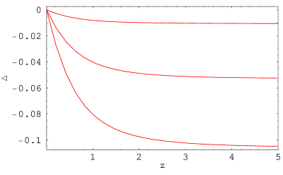
Figure 1: $\Delta\equiv\Delta\alpha/\alpha$ vs. $z$ for $n=6$ and $\zeta_{F}=-2$ with various initial conditions $\varphi_{i}=-0.01$, $-0.05$, and $-0.1$, from top to bottom.

In the early radiation era, $\phi$ may be displaced from $\overline{\phi}$ and “frozen” due to the large frictional term $3H\dot{\phi}$ in the evolution equation. However, for nonzero $m\sim H_{0}$, the magnitude of the initial value $|\varphi_{i}|$ in the early radiation era must still be $\ll 1$ to satisfy the BBN, CMB, and quasar bounds on the variation of $\alpha$. To see this, note that for $m\sim H_{0}$, $\varphi$ is frozen near $\varphi_{i}$ until $H$ becomes of order $H_{0}$ and then decays with a characteristic timescale on the order of $H_{0}^{-1}$. Thus the change in $\varphi$ from the early radiation era to the present and the concomitant change $\Delta\alpha/\alpha$ are on the order of $\varphi_{i}$ (see Fig. 1). To satisfy the quasar bounds on $\Delta\alpha/\alpha$ would require fine tuning of initial conditions ($\varphi_{i}\approx-10^{-5}$).

For $m=0$, the initial condition for $\varphi$ is irrelevant in the linearized theory (6) since $\Delta\alpha$ only depends on changes in $\varphi$; the value of $\varphi_{i}$ becomes important only if the scalar potential cannot be neglected.

It is plausible though that $\varphi=0$ in the early radiation era, since $V(\phi)$ may have a deep minimum at $\overline{\phi}$ during inflation in the very early universe, which later, after one or more phase transitions, becomes shallow with $V^{\prime\prime}(\overline{\phi})\sim H_{0}$. For example, in the primordial inflationary stage, $V^{\prime\prime}(\overline{\phi})$ may be on the order of $H_{I}^{2}$, where $H_{I}\gg H_{0}$ is the Hubble parameter during primordial inflation. While the scale factor $a$ inflates by 60 or more e-foldings, $\phi$ will in this scenario rapidly approach $\overline{\phi}$. We therefore take $\varphi=0=\dot{\varphi}$ in the early radiation era.

Equation (6) may be put into dimensionless form by setting $\tau=H_{\Lambda}t=\Omega_{\Lambda}^{1/2}H_{0}t$:

$$\ddot{\varphi}+3\frac{H}{H_{\Lambda}}\dot{\varphi}+n\varphi=-3\zeta\frac{\Omega_{m}}{\Omega_{\Lambda}}\left(\frac{a_{0}}{a}\right)^{3}$$ (14)

where henceforth a dot over $\varphi$ denotes differentiation with respect to $\tau$.

The Hubble parameter is related to the scale factor and the energy densities in matter, radiation, and the cosmological constant through the Friedmann equation

$$\frac{H^{2}}{H_{\Lambda}^{2}}=\left(\frac{1}{a}\frac{da}{d\tau}\right)^{2}=\frac{\Omega_{m}}{\Omega_{\Lambda}}\left(\frac{a_{0}}{a}\right)^{3}+\frac{\Omega_{r}}{\Omega_{\Lambda}}\left(\frac{a_{0}}{a}\right)^{4}+1$$ (15)

which can be used to solve for $a$ and $H$ in the matter-$\Lambda$, early matter, and radiation eras.

In the matter-$\Lambda$ era, the scale factor and Hubble parameter have the explicit forms

$$\frac{a}{a_{0}}=\frac{1}{1+z}=\left(\frac{\Omega_{m}}{\Omega_{\Lambda}}\right)^{1/3}\sinh^{2/3}\left(\frac{3}{2}\tau\right)$$ (16)

$$H=H_{\Lambda}\coth\left(\frac{3}{2}\tau\right)$$ (17)

and the evolution equation becomes

$$\ddot{\varphi}+3\coth\left(\frac{3}{2}\tau\right)\dot{\varphi}+n\varphi=\frac{-3\zeta}{\sinh^{2}\left(\frac{3}{2}\tau\right)}~{}.$$ (18)

In the early matter era, the scale factor

$$\frac{a}{a_{0}}\approx\left(\frac{\Omega_{m}}{\Omega_{\Lambda}}\right)^{1/3}\left(\frac{3\tau}{2}\right)^{2/3}$$ (19)

and the Hubble parameter $H/H_{\Lambda}\approx 2/(3\tau)$. The mass term $n\varphi$ in Eq. (14) can be neglected in the early matter (and radiation) eras. The evolution equation for the scalar field in the early matter era becomes

$$\ddot{\varphi}+\frac{2}{\tau}\dot{\varphi}=-\frac{4\zeta}{3\tau^{2}}$$ (20)

which has the solution

$$\varphi_{m}=-\frac{4\zeta}{3}\left(\ln\frac{\tau}{\tau_{m-r}}+\frac{c_{1}}{\tau}+c_{2}\right)$$ (21)

where $\tau_{m-r}=H_{\Lambda}t_{m-r}$ and $c_{1}$ and $c_{2}$ are constants of integration.

In the radiation era, the scale factor

$$\frac{a}{a_{0}}\approx\left(\frac{4\Omega_{r}}{\Omega_{\Lambda}}\right)^{1/4}s^{1/2},~{}~{}s=\tau-\frac{\tau_{m-r}}{4}$$ (22)

and the Hubble parameter $H/H_{\Lambda}\approx 1/(2s)$. The time shift $\tau_{m-r}/4$ is determined by matching the Hubble parameters from the radiation and early matter eras at $\tau_{m-r}$. (The formal mathematical singularity at $a\rightarrow 0$ now occurs at $t=t_{m-r}/4$ due to the choice of the zero of time in Eq. (16).) The evolution equation for the scalar field becomes

$$\ddot{\varphi}+\frac{3}{2s}\dot{\varphi}=\frac{-3\zeta}{4s_{m-r}^{1/2}s^{3/2}}~{}.$$ (23)

The solution in the radiation era is

$$\varphi_{r}=-\frac{3\zeta}{2}\left(\frac{s^{1/2}}{s_{m-r}^{1/2}}+\frac{c_{3}}{s^{1/2}}+c_{4}\right)$$ (24)

where $c_{3}$ and $c_{4}$ are constants of integration.

The initial conditions for the scalar field in the early radiation era are $\varphi_{r}(\tau_{i})=0=\dot{\varphi}_{r}(\tau_{i})$, where the initial time $\tau_{i}$ satisfies $s_{i}\ll s_{m-r}$. These initial conditions fix the constants in the solution (24), yielding

$$\varphi_{r}=-\frac{3\zeta}{2}\left(\frac{s^{1/2}}{s_{m-r}^{1/2}}+\frac{s_{i}}{s_{m-r}^{1/2}s^{1/2}}-\frac{2s_{i}^{1/2}}{s_{m-r}^{1/2}}\right)~{}.$$ (25)

Next take the limit $s_{i}/s_{m-r}\rightarrow 0$ to obtain

$$\varphi_{r}\approx-\frac{3\zeta}{2}\frac{s^{1/2}}{s_{m-r}^{1/2}}~{}.$$ (26)

Now match $\varphi_{r}=\varphi_{m}$ and $\dot{\varphi}_{r}=\dot{\varphi}_{m}$ at $\tau_{m-r}$ to determine the constants in the solution (21):

$$\varphi_{m}=-\frac{4\zeta}{3}\left(\ln\frac{\tau}{\tau_{m-r}}+\frac{\tau_{m-r}}{4\tau}+\frac{7}{8}\right)$$ (27)

$$\dot{\varphi}_{m}=-\frac{4\zeta}{3}\left(\frac{1}{\tau}-\frac{\tau_{m-r}}{4\tau^{2}}\right)~{}.$$ (28)

To simulate the evolution of the scalar field in the matter-$\Lambda$ era, we use Eq. (18) with initial conditions provided by Eqs. (27) and (28) evaluated at $\tau_{m-r}$.

4 Comparison with Quasar, Meteorite, and Oklo Data

In numerical values for expressions, we take $\Omega_{m}$ = 0.27, $\Omega_{\Lambda}$ = 0.73, and $H_{0}$ = 71 (km/sec)/Mparsec = $1.5\times 10^{-33}$ eV, from Table 10 of the first-year WMAP observations [26]. With these parameters, the age of the universe is $t_{0}$ = 13.7 Gyrs, and the absorption clouds at $z$ = 0.2–3.7 date to 2.4–11.9 Gyrs ago.

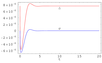
Figure 2: Scalar field $\varphi$ and $\Delta\alpha/\alpha$ vs. $t/t_{0}$ for $n=6$.

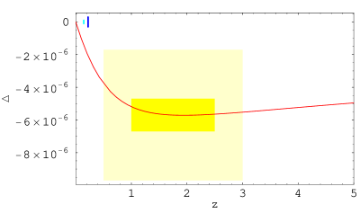
Figure 3: $\Delta\alpha/\alpha$ vs. $z$ for $n=6$.

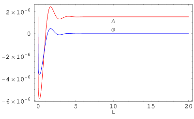
Figure 4: Scalar field $\varphi$ and $\Delta\alpha/\alpha$ vs. $t/t_{0}$ for $n=12$.

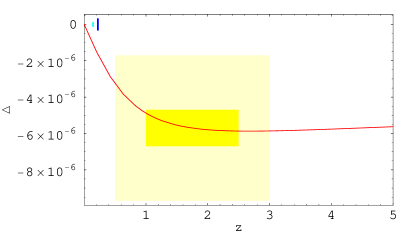
Figure 5: $\Delta\alpha/\alpha$ vs. $z$ for $n=12$.

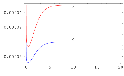
Figure 6: Scalar field $\varphi$ and $\Delta\alpha/\alpha$ vs. $t/t_{0}$ for $n=2$.

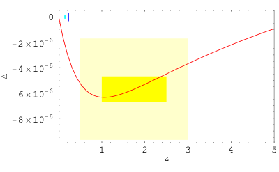
Figure 7: $\Delta\alpha/\alpha$ vs. $z$ for $n=2$.

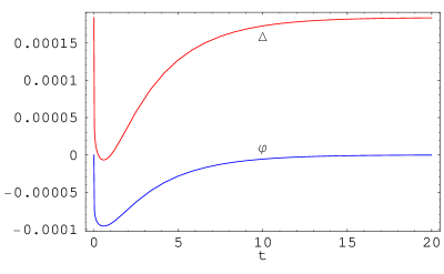
Figure 8: Scalar field $\varphi$ and $\Delta\alpha/\alpha$ vs. $t/t_{0}$ for $n=1$.

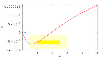
Figure 9: $\Delta\alpha/\alpha$ vs. $z$ for $n=1$.

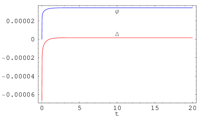
Figure 10: Scalar field $\varphi$ and $\Delta\alpha/\alpha$ vs. $t/t_{0}$ for $n=0$.

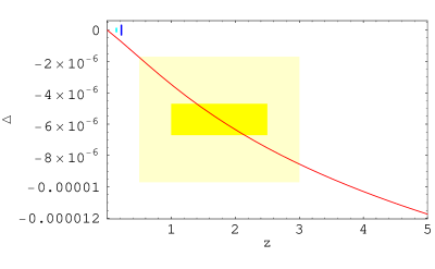
Figure 11: $\Delta\alpha/\alpha$ vs. $z$ for $n=0$.

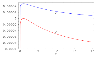
Figure 12: Scalar field $\varphi$ and $\Delta\alpha/\alpha$ vs. $t/t_{0}$ for $n=0.3$.

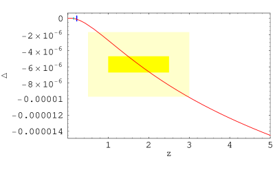
Figure 13: $\Delta\alpha/\alpha$ vs. $z$ for $n=0.3$.

Figs. 2–13 present simulations of the evolution of the scalar field and $\Delta\alpha/\alpha$ for $n$ = 6, 12, 2, 1, 0, and 0.3.

In the figures for $\Delta\alpha(z)/\alpha$, the dark (1 $\sigma$ error bounds for $1\leq z\leq 2.5$) and light (a rough guide to the error bars for $0.6\leq z\leq 3$) boxes indicate the quasar bounds from the bottom panel of Fig. 2 of Ref. [2], while the short vertical lines at $z=0.14$ and $z=0.44/2$ indicate the Oklo and approximate meteorite bounds respectively. While the Oklo event is sharply located in time, the ratio of ¹⁸⁷Re to ¹⁸⁷Os observed today in meteorites involves the total change in $\alpha$ since the time of formation of the meteorites, which is calculated by averaging $\alpha-\alpha_{0}$:

$$\left(\frac{\Delta\alpha}{\alpha}\right)_{meteor}=\frac{1}{t_{0}-t}\int_{t}^{t_{0}}\frac{\alpha(s)}{\alpha_{0}}ds-1~{}.$$ (29)

The scalar field $\varphi$ solving the initial value problem defined in Eqs. (18), (27), and (28) will be proportional to $\zeta$, and thus $\Delta\alpha/\alpha$ will be proportional to $\zeta\zeta_{F}$. For simplicity we will set $\zeta_{F}=-2$, but a general value for $\zeta_{F}$ can be reinserted. For $0\leq n\leq 12$ except $n=1$, $\zeta$ is fixed by setting $\Delta\alpha/\alpha=-0.57\times 10^{-5}$ at $z$ = 1.75. For $n=1$, better results were obtained by setting $\Delta\alpha/\alpha=-0.57\times 10^{-5}$ at $z$ = 1 (see Fig. 9). The massless case shown in Fig. 10 agrees with Eq. (3.4) of Ref. [12] with $\zeta_{\Lambda}=0$. For $n=0.3$, Figs. 13 and 14 show that the quasar, meteorite, and Oklo bounds can be satisfied simultaneously.

The number of visible oscillations in the scalar field $\varphi$ (and thus also in $\Delta\alpha/\alpha$) corresponds to how massive the scalar field is, with at one extreme no oscillations for the massless case (Fig. 10), and at the other extreme two visible oscillations for the $n$ = 12 case (Fig. 4).

In this model, for $n>1$ ($n=1$), $\alpha$ was actually larger in the past at some point before the period of the $z$ = 0.2–3.7 ($z$ = 0.2–1.9) absorption clouds, and will be larger again in the future. For $n=0$, $\alpha$ was smaller in the past, but will be very slightly larger in the future. And for $n=0.3$, $\alpha$ was smaller in the past until just after $t_{Oklo}$, was slightly larger from that point up to $t_{0}$, and then again will be smaller in the future ($\Delta\alpha/\alpha\rightarrow-10^{-4}$).

Values of $\zeta$, BBN, CMB, meteorite, and Oklo $\Delta\alpha/\alpha$, and $(\dot{\alpha}/\alpha)_{0}$ for various scalar field masses are presented in Table 1.

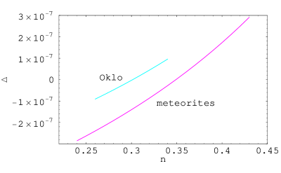
Figure 14: $\Delta\alpha/\alpha$ vs. $n$ satisfying the Oklo and meteorite bounds.

The BBN, CMB, and quasar bounds on $\Delta\alpha/\alpha$ and the laboratory bound on $|\dot{\alpha}/\alpha|_{0}$ are satisfied for integer $0\leq n\leq 12$, except that the $n=1$ case cannot be made to satisfy the quasar bounds in this model. The variation $|\Delta\alpha/\alpha|$ satisfies in addition the Oklo bound for $0.26\leq n\leq 0.34$ and the meteorite bound for $0.24\leq n\leq 0.43$ (see Fig. 14). There is a small range of scalar field masses for which $|\Delta\alpha/\alpha|_{Oklo}<10^{-8}$ (and can be made to go to zero by extreme fine tuning). For this range of $n$, $(\Delta\alpha/\alpha)_{meteor}\approx-1\times 10^{-7}$.

Depending on the scalar field mass, the predicted BBN, CMB, meteorite, and Oklo values of $\alpha$ may be slightly smaller or larger than $\alpha_{0}$. Note that the sign of $\zeta$ for $n=0$ is opposite to the sign for $n\geq 1$. An order of magnitude improvement in the experimental technique could lead to a detection of $(\dot{\alpha}/\alpha)_{0}$.

For the massless case, the variation in $\alpha$ can be made marginally consistent with the quasar, meteorite, and Oklo bounds by setting $\Delta\alpha/\alpha=-0.18\times 10^{-5}$ at $z$ = 3 (Fig. 15).

The behavior of $\alpha(z)$ can pin down the values for $\zeta$ and $m$. Conversely, even knowing only the sign of $\zeta$ or $\Delta\alpha/\alpha$ can rule out certain values of the scalar field mass. For example, if $(\Delta\alpha/\alpha)_{BBN}>0$ or $\zeta\zeta_{F}<0$, then $n\stackrel{{\scriptstyle>}}{{\mbox{\scriptsize$\sim$}}}1$.

5 Conclusion

Asymptotically $\alpha(t)$ in this model goes to a constant value $\overline{\alpha}\approx\alpha_{0}$ in the early radiation and the late $\Lambda$ dominated eras. The coupling of the scalar field to (nonrelativistic) matter drives $\alpha$ slightly away from $\overline{\alpha}$ in the epochs when the density of matter is important.

Even for $\Omega_{\Lambda}=0$, $\alpha\rightarrow\overline{\alpha}$ as $t\rightarrow\infty$ as long as $m\neq 0$. In the massless case, as $t\rightarrow\infty$, $\alpha$ goes to a constant value which differs from $\overline{\alpha}$ but still approximately equals 1/137 for $\Omega_{\Lambda}>0$, while if $\Omega_{\Lambda}=0$ (and $V(\phi)\equiv 0$), $\Delta\alpha\sim\zeta\zeta_{F}\ln(\tau/\tau_{0})$, as in Ref. [11]. Thus the variation $|\Delta\alpha/\alpha|$ of the fine structure constant becomes of order 1 only if both $\rho_{\Lambda}\rightarrow 0$ and $m=0$, and only for $t\gg t_{0}$.

The simulations above indicate that it is possible to extract properties of the scalar field from quasar absorption line spectra, including the coupling of $\phi$ to matter and its mass. The variation of $\alpha$ has different behaviors in the redshift range $0\leq z\leq 5$ depending on the mass of the scalar field. Thus additional quasar absorption line data, and better Oklo and meteorite bounds, will help elucidate the properties of the scalar field. The case $m=H_{\Lambda}$ is ruled out in this model. A laboratory detection of $(\dot{\alpha}/\alpha)_{0}$ may be possible in the near future.

To satisfy the quasar, meteorite, and Oklo bounds on $\Delta\alpha/\alpha$, the mass of the scalar field has to be on the order of 0.5–0.6 $H_{\Lambda}$. It is difficult to satisfy both the Oklo/meteorite and quasar bounds in theories where the variation of $\alpha$ derives from the evolution of a scalar field; the scalar field in the model studied here must be near an extremum near $t_{Oklo}$ and $t_{0}$.

The key insight of this model, as well as other models of variable $\alpha$, is that variation of $\alpha$ provides a window into the parameters of the underlying theory that unifies gravity and the standard model of particle physics.

$n$	$\zeta$	$(\Delta\alpha/\alpha)_{BBN}$	$(\Delta\alpha/\alpha)_{CMB}$	$(\Delta\alpha/\alpha)_{meteor}$	$(\Delta\alpha/\alpha)_{Oklo}$	$(\dot{\alpha}/\alpha)_{0}$
0	$-2.0\times 10^{-6}$	$-6.7\times 10^{-5}$	$-5.3\times 10^{-5}$	$-6.8\times 10^{-7}$	$-4.8\times 10^{-7}$	$2.4\times 10^{-16}$
0.3	$-3.0\times 10^{-6}$	$-9.6\times 10^{-5}$	$-7.6\times 10^{-5}$	$-1.4\times 10^{-7}$	$-3.2\times 10^{-9}$	$-6.8\times 10^{-17}$
0.31	$-3.0\times 10^{-6}$	$-9.8\times 10^{-5}$	$-7.7\times 10^{-5}$	$-1.1\times 10^{-7}$	$2.0\times 10^{-8}$	$-8.3\times 10^{-17}$
1	$6.1\times 10^{-6}$	$1.8\times 10^{-4}$	$1.4\times 10^{-4}$	$-3.7\times 10^{-6}$	$-3.2\times 10^{-6}$	$2.0\times 10^{-15}$
2	$1.9\times 10^{-6}$	$5.0\times 10^{-5}$	$3.8\times 10^{-5}$	$-2.7\times 10^{-6}$	$-2.2\times 10^{-6}$	$1.3\times 10^{-15}$
3	$1.0\times 10^{-6}$	$2.4\times 10^{-5}$	$1.7\times 10^{-5}$	$-2.2\times 10^{-6}$	$-1.8\times 10^{-6}$	$1.1\times 10^{-15}$
4	$7.0\times 10^{-7}$	$1.5\times 10^{-5}$	$1.0\times 10^{-5}$	$-2.0\times 10^{-6}$	$-1.6\times 10^{-6}$	$9.3\times 10^{-16}$
6	$4.6\times 10^{-7}$	$7.6\times 10^{-6}$	$4.4\times 10^{-6}$	$-1.8\times 10^{-6}$	$-1.4\times 10^{-6}$	$8.0\times 10^{-16}$
12	$2.6\times 10^{-7}$	$1.5\times 10^{-6}$	$-2.8\times 10^{-7}$	$-1.4\times 10^{-6}$	$-1.1\times 10^{-6}$	$5.7\times 10^{-16}$

Table 1: Values of $\zeta$, BBN, CMB, meteorite, and Oklo $\Delta\alpha/\alpha$, and $(\dot{\alpha}/\alpha)_{0}$ in yr^-1 vs. scalar field mass squared $n$.

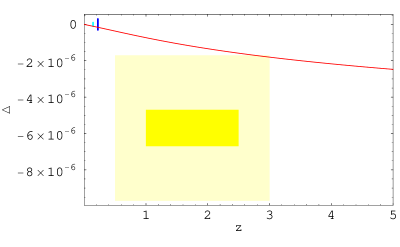
Figure 15: $\Delta\alpha/\alpha$ vs. $z$ for $n=0$ by setting $\Delta\alpha/\alpha=-0.18\times 10^{-5}$ at $z$ = 3.

References

- [1] J. K. Webb, M. T. Murphy, V. V. Flambaum, V. A. Dzuba, J. D. Barrow, C. W. Churchill, J. X. Prochaska, and A. M. Wolfe, Phys. Rev. Lett. 87, 091301 (2001), astro-ph/0012539.
- [2] J. K. Webb, M. T. Murphy, V. V. Flambaum, and S. J. Curran, Astrophys. Space Sci. 283, 565 (2003), astro-ph/0210531.
- [3] J. P. Uzan, Rev. Mod. Phys. 75, 403 (2003), hep-ph/0205340.
- [4] A. I. Shlyakhter, Nature (London) 264, 340 (1976).
- [5] T. Damour and F. Dyson, Nucl. Phys. B 480, 37 (1996), hep-ph/9606486.
- [6] K. A. Olive, M. Pospelov, Y.-Z. Qian, A. Coc, M. Cassé, and E. Vangioni-Flam, Phys. Rev. D 66, 045022 (2002), hep-ph/0205269.
- [7] J. D. Prestage, R. L. Tjoelker, and L. Maleki, Phys. Rev. Lett. 74, 3511 (1995).
- [8] H. Marion et al., Phys. Rev. Lett. 90, 150801 (2003), physics/0212112.
- [9] J. D. Bekenstein, Phys. Rev. D 25, 1527 (1982).
- [10] H. B. Sandvik, J. D. Barrow, and J. Magueijo, Phys. Rev. Lett. 88, 031302 (2002), astro-ph/0107512.
- [11] J. D. Barrow, H. B. Sandvik, and J. Magueijo, Phys. Rev. D 65, 063504 (2002), astro-ph/0109414.
- [12] K. A. Olive and M. Pospelov, Phys. Rev. D 65, 085044 (2002), hep-ph/0110377.
- [13] T. Damour and A. M. Polyakov, Nucl. Phys. B 423, 532 (1994), hep-th/9401069.
- [14] T. Damour, G. W. Gibbons, and C. Gundlach, Phys. Rev. Lett. 64, 123 (1990).
- [15] T. Damour, gr-qc/0306023.
- [16] S. J. Gates and B. Zwiebach, Phys. Lett. B 123, 200 (1983).
- [17] C. M. Hull and N. P. Warner, Class. Quant. Grav. 5, 1517 (1988).
- [18] R. Kallosh, A. D. Linde, S. Prokushkin, and M. Shmakova, Phys. Rev. D 65, 105016 (2002), hep-th/0110089.
- [19] G. W. Gibbons and C. M. Hull, hep-th/0111072.
- [20] P. Fré, M. Trigiante, and A. Van Proeyen, Class. Quant. Grav. 19, 4167 (2002), hep-th/0205119.
- [21] R. Kallosh, hep-th/0205315.
- [22] R. Kallosh, A. D. Linde, S. Prokushkin, and M. Shmakova, Phys. Rev. D 66, 123503 (2002), hep-th/0208156.
- [23] R. Kallosh and A. D. Linde, Phys. Rev. D 67, 023510 (2003), hep-th/0208157.
- [24] T. Damour, F. Piazza, and G. Veneziano, Phys. Rev. Lett. 89, 081601 (2002), gr-qc/0204094.
- [25] T. Damour, F. Piazza, and G. Veneziano, Phys. Rev. D 66, 046007 (2002), hep-th/0205111.
- [26] D. N. Spergel et al., astro-ph/0302209.