Observing the Reionization Epoch Through 21 Centimeter Radiation

Abstract

We study the observability of the reionization epoch through the 21 cm hyperfine transition of neutral hydrogen. We use a high-resolution cosmological simulation (including hydrodynamics) together with a fast radiative transfer algorithm to compute the evolution of 21 cm emission from the intergalactic medium (IGM) in several different models of reionization. We show that the mean brightness temperature of the IGM drops from $\delta T_{b}\sim 25\mbox{ mK}$ to $\delta T_{b}\sim 10^{-2}\mbox{ mK}$ during overlap (over a frequency interval $\Delta\nu\sim 25\mbox{ MHz}$), while the root mean square fluctuations on small scales drop abruptly from $\langle\delta T_{b}^{2}\rangle^{1/2}\sim 10\mbox{ mK}$ to $\langle\delta T_{b}^{2}\rangle^{1/2}\sim 10^{-1}\mbox{ mK}$ at the end of overlap. We show that 21 cm observations can efficiently discriminate models with a single early reionization epoch from models with two distinct reionization episodes.

1 Introduction

One of the major challenges in cosmology is to understand the first phases of structure formation. We do not yet know whether early generations of sources were similar to galaxies and quasars in the local universe or qualitatively different from them (and if so, in what ways). Because these sources affect the formation of all subsequent generations of luminous objects, understanding their characteristics is critical to any theory of structure formation. In many ways, the defining event of this era is “reionization,” when the first sources of light ionized hydrogen in the intergalactic medium (IGM). The timing of this event, and its morphological evolution, contains a wealth of information about these first sources and about the IGM itself (e.g., Wyithe & Loeb 2003b; Cen 2003; Haiman & Holder 2003; Mackey et al. 2003; Yoshida et al. 2003a, b).

Observational constraints on this epoch are difficult to obtain, but those that do exist are intriguing. The most straightforward way to study the ionization state of the IGM is through quasar absorption spectra: regions with relatively large HI densities appear as absorption troughs in the quasar spectra, creating a “Ly$\alpha$ forest” of absorption lines. Spectra of $z\sim 6$ quasars selected from the Sloan Digital Sky Survey (SDSS) not only show at least one extended region of zero transmission (Becker et al., 2001) but also imply that the ionizing background is rising rapidly at this time (Fan et al., 2002). Both of these results are consistent with a scenario in which reionization ends at $z_{r}\sim 6$. Another constraint comes from measuring the fraction of the cosmic microwave background (CMB) radiation that has been Thomson scattered by ionized gas in the IGM. Recent observations made by the Wilkinson Microwave Anisotropy Probe (WMAP) imply that reionization occurred at $z_{r}\ga 14$ (Kogut et al., 2003; Spergel et al., 2003). Finally, measurements of the temperature of the Ly$\alpha$ forest at $z\sim 2$–$4$ suggest an order unity change in the ionized fraction at $z_{r}\la 10$ (Theuns et al., 2002; Hui & Haiman, 2003), although this argument is subject to important uncertainties about HeII reionization (e.g., Sokasian et al. 2002). Reconciling these different observations implies that sources must exhibit substantial (perhaps qualitative) evolution between high redshifts and the present day (Sokasian et al., 2003; Wyithe & Loeb, 2003b; Cen, 2003; Haiman & Holder, 2003). A better understanding of reionization has the potential to teach us the detailed evolutionary history of luminous sources.

Unfortunately, learning much more from these observations promises to be difficult. The optical depth of the IGM to Ly$\alpha$ absorption is $\tau_{\alpha}\approx 6.45\times 10^{5}x_{\rm HI}[(1+z)/10]^{3/2}$ (Gunn & Peterson, 1965), where $x_{\rm HI}$ is the neutral fraction and where we have assumed the currently favored cosmological parameters (see below). A neutral fraction $x_{\rm HI}\ga 10^{-3}$ will therefore render the absorption trough completely black; quasar absorption spectra can clearly probe only the very late stages of reionization. CMB measurements, on the other hand, depend on the ionized gas density and thus are most sensitive to the early stages of reionization. However, existing observations essentially provide only an integral constraint on the ionized gas column; distinguishing different reionization histories with CMB observations alone promises to be quite challenging (Holder et al., 2003).

It is therefore crucial to develop other probes of the high-redshift IGM. One possibility is to observe a transition much weaker then Ly$\alpha$. Perhaps the most interesting candidate is the 21 cm hyperfine line of neutral hydrogen in the IGM (Field, 1958, 1959a). The physics of the 21 cm transition has been well-studied in the cosmological context (e.g., Scott & Rees 1990; Kumar et al. 1995; Madau et al. 1997; Chen & Miralda-Escudé 2003). There are three methods to study the IGM through this line. First, we can search for emission or absorption from the diffuse IGM and condensed minihaloes (i.e., collapsed objects that are unable to cool and form stars) at high redshifts. While the absolute signal from this gas will be swamped by foreground emission, the signal on the sky will fluctuate because of variations in the IGM density and neutral fraction (Madau et al., 1997; Tozzi et al., 2000; Iliev et al., 2002). Second, we can seek a global (all sky) signature when the neutral emitting gas is destroyed. Assuming that reionization occurs rapidly, this will appear as a “step” in the otherwise smooth low-frequency radio spectrum of the sky (Shaver et al., 1999). Third, high-resolution spectra of powerful radio sources at high-redshifts will reveal absorption features caused by sheets, filaments, and minihaloes in the neutral IGM (Carilli et al., 2002; Furlanetto & Loeb, 2002).

To date, predictions about the 21 cm signal of the diffuse IGM near the epoch of reionization have been difficult to obtain. This is because such predictions require a careful treatment of ionizing sources and radiative transfer in order to describe adequately the transition from a neutral to an ionized medium. Only recently has it become possible to combine numerical radiative transfer schemes with cosmological simulations in order to study this process in detail (Gnedin, 2000; Razoumov et al., 2002; Ciardi et al., 2003; Sokasian et al., 2003). As shown by Ciardi & Madau (2003), such simulations allow us, for the first time, to realistically model the behavior of 21 cm IGM emission. In this paper, we analyze the simulations of Sokasian et al. (2003) in order to quantify the 21 cm emission expected before, during, and after reionization. We focus purely on the emission signal because absorption studies require careful treatment of both ultraviolet radiation (above and below the Lyman limit) and X-ray photons (Chen & Miralda-Escudé, 2003), which is extremely difficult (see Carilli et al. 2002 for a first attempt). We study scenarios in which the IGM is reionized once (at either early or late times) as well as “double reionization” histories that may reconcile the SDSS and WMAP observations (Wyithe & Loeb, 2003b; Cen, 2003). We show that 21 cm measurements offer a promising route for distinguishing reionization scenarios that would appear identical in CMB and quasar observations.

We briefly describe our cosmological simulations and reionization models in §2. We then discuss the physics of 21 cm emission, and our analysis procedure, in §3. We present our results in §4 and discuss their observability and their implications for understanding reionization scenarios in §5.

2 Simulations

All of our calculations are performed within the Q5 cosmological simulation of Springel & Hernquist (2003b). This smoothed-particle hydrodynamics (SPH) simulation uses a modified version of the GADGET code (Springel et al., 2001) incorporating a new conservative formulation of SPH with the specific entropy as an independent variable (Springel & Hernquist, 2002). The simulation also includes a new description of star formation and feedback in the interstellar medium of galaxies (Springel & Hernquist, 2003a). Within the extended series of simulations performed by Springel & Hernquist (2003b), this model yields a converged prediction for the cosmic star formation rate. Using simple physical arguments, Hernquist & Springel (2003) have shown that the star formation rate density evolves according to:

$$\dot{\rho}_{\star}=\dot{\rho}_{\star}(0)\frac{\chi^{2}}{1+\alpha(\chi-1)^{3}\exp(\beta\chi^{7/4})},$$ (1)

where

$$\chi(z)=\left(\frac{H(z)}{H_{0}}\right)^{2/3}.$$ (2)

Here the constants $\alpha=0.012$, $\beta=0.041$, and $\dot{\rho}_{\star}(0)=0.013\mbox{ M${}_{\odot}$ yr${}^{-1}$ Mpc${}^{-3}$}$ are chosen by fitting the simulation results of Springel & Hernquist (2003b). The form of the function is motivated by two competing processes affecting the total star formation rate. At high redshifts, when cooling times are short, star formation is only limited by the growth of massive haloes. At low redshifts, cooling times become long because of the expansion of the universe; thus in this regime the star formation rate density evolves primarily because of the expansion of the universe.

The simulation assumes a $\Lambda$CDM cosmology with $\Omega_{m}=0.3$, $\Omega_{\Lambda}=0.7$, $\Omega_{b}=0.04$, $H_{0}=100h\mbox{ km s${}^{-1}$ Mpc${}^{-1}$}$ (with $h=0.7$), and a scale-invariant primordial power spectrum with index $n=1$ normalized to $\sigma_{8}=0.9$ at the present day. These parameters are consistent with the most recent cosmological observations (e.g., Spergel et al. 2003). The particular simulation we choose has $324^{3}$ dark matter particles and $324^{3}$ SPH particles in a box with sides of $10h^{-1}$ comoving Mpc, yielding particle masses of $2.12\times 10^{6}h^{-1}\mbox{ M${}_{\odot}$}$ and $3.26\times 10^{5}h^{-1}\mbox{ M${}_{\odot}$}$ for the dark matter and gas components, respectively.

The radiative transfer is fully described in Sokasian et al. (2001), so we outline only its most significant aspects here. We perform the adiative transfer on a Cartesian grid with $200^{3}$ cells using an adaptive ray-casting scheme (Abel & Wandelt, 2002). Density fields, clumping factors, and source characteristics are taken from outputs of the hydrodynamic simulations. Thus, the radiative transfer is done in a post-processing step after the simulations have been completed, and we neglect the dynamical feedback of the radiation on structure formation. We turn off periodic boundary conditions for the radiation once the ionized volume exceeds a certain level. After this time we add photons that reach the edge of the box to a diffuse background. The calculation follows the reionization of both hydrogen and helium. Because ionizing radiation from small galaxies has a substantial effect on reionization, we select sources aggressively (including all groups of 16 or more dark matter particles). At each redshift, we correct the star formation rates in low-mass haloes to match the converged prediction of Hernquist & Springel (2003).

Because the source and IGM properties are determined self-consistently by the simulation, the major unknown parameter in simulations of reionization is the efficiency with which each galaxy produces ionizing photons. This parameter includes two physical effects: the intrinsic rate at which newly formed stars create ionizing photons and the fraction of such photons that are able to escape the galaxy. As a fiducial value, we assume an intrinsic ionizing photon production rate of $\dot{N}_{i,{\rm fid}}\equiv 10^{53}(\dot{M}_{\star}/\mbox{ M${}_{\odot}$ yr${}^{-1}$})\mbox{ s${}^{-1}$}$, where $\dot{M}_{\star}$ is the star formation rate, corresponding to a Salpeter initial mass function (IMF) with solar metallicity. We then set the actual production rate $\dot{N}_{i}=f_{\rm ion}\dot{N}_{i,{\rm fid}}$. Any value $f_{\rm ion}\leq 1$ can be accomodated by the fiducial IMF, while $f_{\rm ion}>1$ will require a change in the IMF. For example, very massive metal-free stars are $\sim 30$ more efficient at creating ionizing photons than “normal” stars (Bromm et al., 2001). Sokasian et al. (2003) found that the choice $f_{\rm ion}=0.2$ matches data from $z\sim 6$ quasars selected through the SDSS (Becker et al., 2001; Djorgovski et al., 2001). However, this model implies an optical depth to Thomson scattering significantly below the limits from recent observations by WMAP. Sokasian et al. (2003) showed that one way to increase the optical depth without destroying the match to the quasar observations is to gradually increase the ionizing efficiency with redshift in the form $f_{\rm ion}(z)=0.20e^{(z-6)/3}$. Such a model achieves overlap at $z\sim 13$. However, because $f_{\rm ion}$ declines rapidly with cosmic time, the statistics of quasar absorbers remain essentially unaffected (i.e., most of the extra high-redshift photons are balanced by recombinations before $z\sim 6$). We note that in this model $f_{\rm ion}>1$ for $z>11$, indicating that the IMF at these redshifts differs from that of local galaxies.

Another way to reconcile the quasar and CMB observations is either partial or complete “double reionization” (Cen, 2002; Wyithe & Loeb, 2003a). In such a scenario, sources reionize the universe at $z\ga 15$. Some form of feedback then prevents these sources from continuing to form and grow, rapidly reducing the production rate of ionizing photons. For example, feedback can either prevent stars from forming in small haloes or change the mode of star formation. (In our notation, $f_{\rm ion}$ essentially changes discontinuously at the moment of overlap.) Because the recombination time at high redshifts is short compared to the Hubble time, much of the universe recombines before “normal” protogalaxies can cause a second reionization event at a later time. Note that, although both smooth and discontinuous increases in $f_{\rm ion}$ produce large optical depths to the CMB, the qualitative evolution of the neutral gas differs markedly between the two models. Unfortunately, our simulation cannot resolve the haloes that are responsible for the first reionization epoch in these scenarios. We therefore introduce an approximate model for double reionization by setting the neutral fraction $x_{\rm HI}=0.01$ throughout the simulation volume for all $z>z_{t}$. At $z=z_{t}$, we allow the gas to recombine. We set $f_{\rm ion}=0.2$ for these two models. Note that the simulation assumes that the ionized gas has $T=5000\mbox{ K}$. If the photoionized gas has a higher initial temperature, recombination may take slightly longer (the recombination time $t_{\rm rec}\propto T^{0.7}$).

We show in Figure 1 the optical depth to Thomson scattering $\tau_{e}$ between the present day and redshift $z$ in these four models. These calculations assume that $x_{\rm HI}=x_{\rm HeI}$ until $z=3$, when helium is instantaneously doubly ionized throughout the universe. The solid curve corresponds to $f_{\rm ion}=0.2$ without an early phase of reionization. The short- and long-dashed curves correspond to our double reionization model, with $z_{t}=14.5$ and $z_{t}=18.4$, respectively. The dot-dashed curve corresponds to the model with variable $f_{\rm ion}(z)$. The horizontal dotted line shows the $2\sigma$ lower limit to $\tau_{e}$ from Kogut et al. (2003). We note that, in the double reionization models, we can always increase $\tau_{e}$ by placing the onset of the initial reionization phase at arbitrarily high redshift. For reference, making the total $\tau_{e}=0.13$ would require the fully ionized phase to begin by $z\sim 18.4$ or $z\sim 22$ if $z_{t}=14.5$ or $z_{t}=18.4$, respectively.

Figure 1: The integrated optical depth to electron scattering $\tau_{e}$ between the present day and redshift $z$. The curves correspond to our different reionization models. The solid curve assumes a constant $f_{\rm ion}=0.2$ for all sources throughout cosmic time. The dot-dashed curve assumes a variable $f_{\rm ion}(z)$ (see text). The short-dashed and long-dashed curves assume $f_{\rm ion}=0.2$ but set $x_{\rm HI}=0.01$ everywhere until $z_{t}=14.5$ and $z_{t}=18.4$, respectively. The horizontal dotted line shows the lower limit to $\tau_{e}$ (at $68\%$ confidence) of Kogut et al. (2003).

3 21 cm Radiation from the Intergalactic Medium

The optical depth of the neutral IGM to redshifted hyperfine absorption is (Field, 1959a)

$$\tau = \frac{3c^{3}h_{P}A_{10}\,n_{\rm HI}}{32\pi k\nu_{0}^{2}\,T_{S}\,H(z)}$$ (3)

$$\approx 6\times 10^{-3}(1+\delta)x_{\rm HI}\left(\frac{T_{\rm CMB}}{T_{S}}\right)\left(\frac{\Omega_{b}h^{2}}{0.02}\right)$$

$$\times\left[\left(\frac{0.3}{\Omega_{m}}\right)\,\left(\frac{1+z}{10}\right)\right]^{1/2}h^{-1}.$$

Here $h_{P}$ is Planck’s constant, $k$ is Boltzmann’s constant, $\nu_{0}=1420.4\mbox{ MHz}$ is the rest-frame hyperfine transition frequency, $A_{10}=2.85\times 10^{-15}\mbox{ s${}^{-1}$}$ is the spontaneous emission coefficient for the transition, $T_{S}$ is the spin temperature of the IGM (i.e., the excitation temperature of the hyperfine transition), $T_{\rm CMB}=2.73(1+z)\mbox{ K}$ is the CMB temperature at redshift $z$, and $n_{\rm HI}$ is the local neutral hydrogen density. In the second equality, we have assumed sufficiently high redshifts such that $H(z)\approx H_{0}\Omega_{m}^{1/2}(1+z)^{3/2}$ (which is well-satisfied in the era we study, $z>6$). We have set $\delta$ equal to the local overdensity and $x_{\rm HI}$ equal to the neutral fraction.

In the absence of collisions and Ly$\alpha$ photon pumping, the HI spin temperature equals the CMB temperature. In this case the IGM will not be visible through the 21 cm transition. However, either of these mechanisms can couple $T_{S}$ to $T_{K}$, the kinetic temperature of the gas (Wouthuysen, 1952; Field, 1958, 1959b). While collisions are only effective at extremely high redshifts or in collapsed regions, Madau et al. (1997) showed that even a relatively small Ly$\alpha$ photon field is sufficient to couple the spin and kinetic temperatures. Ciardi & Madau (2003) show that (in their simulations) this requirement will be easily satisfied for the redshifts of interest. Because our simulation has a roughly similar total emissivity to theirs, we assume that $T_{S}$ and $T_{K}$ are closely coupled throughout.

The visibility of the IGM then depends on its kinetic temperature. If $T_{K}\ll T_{\rm CMB}$, the IGM will appear in absorption against the CMB. However, the IGM will likely be heated shortly after the first sources appear through X-ray, photoionization, and shock heating (e.g., Chen & Miralda-Escudé 2003). Once heating has occurred, the IGM appears in emission at a level nearly independent of $T_{S}$. For simplicity, and because our simulation does not include all of the relevant heating mechanisms (such as X-rays), we assume $T_{S}\gg T_{\rm CMB}$ throughout. At extremely high redshifts, when the first sources are just turning on, the IGM may instead appear in absorption, but this does not affect the main points of our paper. In the limit $T_{S}\gg T_{\rm CMB}$, the observed brightness temperature excess relative to the CMB is (Madau et al., 1997)

$$\delta T_{b} \approx \frac{T_{S}-T_{\rm CMB}}{1+z}\,\tau$$ (4)

$$\approx\, 16\,(1+\delta)x_{\rm HI}\left(\frac{T_{S}-T_{\rm CMB}}{T_{S}}\right)\left(\frac{\Omega_{b}h^{2}}{0.02}\right)$$

$$\times\left[\left(\frac{0.3}{\Omega_{m}}\right)\,\left(\frac{1+z}{10}\right)\right]^{1/2}h^{-1}\mbox{ mK}.$$

To apply equation (4) to our simulation, we first choose a bandwidth $\Delta\nu$ and beamsize $\Delta\theta$. For reference, these correspond to comoving distances

$$L\approx 1.2\left(\frac{\Delta\nu}{0.1\mbox{ MHz}}\right)\left(\frac{1+z}{10}\right)^{1/2}\left(\frac{\Omega_{m}}{0.3}\right)^{-1/2}h^{-1}\mbox{ Mpc}$$ (5)

and

$$2R\approx 1.9\left(\frac{\Delta\theta}{1^{\prime}}\right)\left(\frac{1+z}{10}\right)^{0.2}h^{-1}\mbox{ Mpc}$$ (6)

over the relevant redshift range. We then choose a slice of depth $L$ within the box and divide it into square pixels of width $2R$. We randomly select one of the axes of the box to be the line of sight and randomly select a starting point within the box in that direction. Next, we calculate the total mass of neutral hydrogen contained in each pixel. The radiative transfer code smooths each particle over the SPH kernel and adds the appropriate mass to each cell of the radiative transfer grid. We multiply the total hydrogen mass in each of these cells by the corresponding neutral fraction computed in the simulation and then assign this mass to the appropriate pixel on the sky. Finally, we divide by the mean IGM mass at that redshift and apply equation (4) in order to find the brightness temperature of the pixel. When presenting our results, we always show the average of five such slices: because of large scale structure, a single slice is not necessarily representative of the box as a whole. Note that this procedure neglects peculiar velocities of the gas particles, which would shift some particles into or out of the frequency range we consider. We discuss the effects of this simplification below.

Although an individual IGM feature is too weak to observe, the statistical fluctuations across the sky or in frequency space may be observable, and they contain information about structure formation and the ionization fraction. Equation (4) shows that fluctuations in either the density $\delta$ or neutral fraction $x_{\rm HI}$ of the IGM lead to fluctuations in the brightness temperature observed against the CMB. While the full simulations are necessary in order to compute $x_{\rm HI}$, we can estimate the level of fluctuations due to variations in the overdensity using linear theory. We wish to compute the mass fluctuations inside a cylindrical window, with the axis of the cylinder along the line of sight (Tozzi et al., 2000). The result is (Iliev et al., 2002)

$$\langle\delta T_{b}^{2}\rangle_{\rm est} = \frac{8D^{2}(z)}{\pi^{2}R^{2}L^{2}}\int_{0}^{\infty}dk\frac{P(k)}{k^{2}}$$ (7)

$$\times\int_{0}^{1}\frac{\sin^{2}(kLx/2)}{x^{2}(1-x^{2})}J_{1}^{2}(kR\sqrt{1-x^{2}})$$

$$\times\qquad s(k,x)dx,$$

where $P(k)$ is the power spectrum at the present day (taken from Eisenstein & Hu 1998), $J_{1}(y)$ is the Bessel function of order unity, $D(z)$ is the growth factor at redshift $z$ (normalised to unity at the present day), and $s(k,x)$ corrects for redshift space distortions. In the limit in which $L\gg R$, $s(k,x)=(1+fx^{2})^{2}$, where $f\approx\Omega_{m}^{0.6}$ (Kaiser, 1987). We note here that the Kaiser (1987) correction cannot be applied outside of this limit. If $R\ga L$, the dominant contribution to $\langle\delta T_{b}^{2}\rangle_{\rm est}$ comes from modes with $k^{-1}\sim R\ga L$, while Kaiser’s derivation only applies to modes with $k^{-1}\ll L$. For $R\gg L$, $s(k,x)$ approaches unity. Qualitatively, this occurs because the small-$k$ modes sampled by such a volume are transverse to the line of sight and hence are unaffected by peculiar velocities.

Figure 2: The brightness temperature fluctuations in a neutral IGM as a function of scale at various redshifts, assuming a bandwidth $\Delta\nu=0.1\mbox{ MHz}$. The solid curves show the root mean square fluctuation from the simulation assuming a fully neutral IGM. The dashed curve shows the estimate from equation (7) with $s(k,x)=1$. The dotted curve shows the estimate with the Kaiser (1987) redshift space correction applied to all scales (see text).

We show how our simulation results compare to this estimate in Figure 2. In each panel, the solid line shows the simulation results for the root mean square fluctuation assuming a fully neutral IGM, while the dashed line shows the estimate of equation (7) with $s(k,x)=1$ (i.e., ignoring peculiar velocity information, as we do in our simulation analysis). We see that equation (7) provides a remarkably good estimate over this entire redshift range. Note that the simulation results steepen slightly with cosmic time, while the shape of the estimate is fixed [the only redshift dependence is in the growth factor $D(z)$, which is independent of scale]. The steepening thus reflects nonlinear structure formation. The simulation results begin to drop steeply for $\Delta\theta>1^{\prime}$, indicating that the simulation cannot fully capture fluctuations on these scales. This is not surprising considering that the box subtends only $\theta_{\rm box}\sim 5^{\prime}$. Comparison to equation (7) also shows that we underestimate the fluctuations for bandwidths $\Delta\nu\ga 0.5\mbox{ MHz}$. We focus on scales $\Delta\theta\la 1^{\prime}$ and $\Delta\nu\la 0.1\mbox{ MHz}$ in most of the following.

Figure 2 also illustrates how the inclusion of peculiar velocities would affect our results. The dotted line shows the estimate of equation (7) with the linear theory redshift-space correction of Kaiser (1987) applied blindly to all $k$-modes. The fluctuation signal increases by $\sim 25\%$. Of course, with our choice of $\Delta\nu$, this correction rigorously only applies for $\Delta\theta\ll 1^{\prime}$, and redshift space distortions will in reality vanish as $\Delta\theta$ increases. The dotted lines therefore actually overestimate the effect of peculiar velocities. We see that peculiar velocities will not affect our qualitative results, so we chose not to complicate the analysis by including them. As a result, we underestimate the fluctuations by $\la 25\%$ for angular scales small compared to the bandwidth.

4 Results

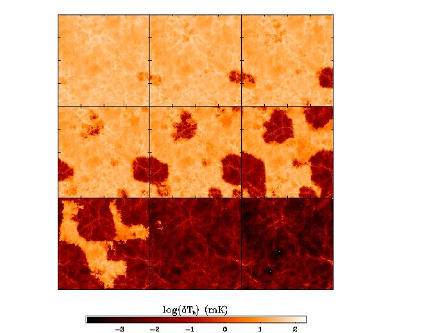
Figure 3: The brightness temperature from the 21 cm transition at various redshifts in the $f_{\rm ion}=0.2$ model and with a bandwidth $\Delta\nu=0.1\mbox{ MHz}$. Each panel corresponds to the same slice of the simulation (of width $10h^{-1}$ comoving Mpc), at $z=12.1$, 11.2, 10.4, 9.8, 9.2, 8.7, 8.3, 7.9, and 7.6, from top left to bottom right.

Figure 3 shows maps of the IGM brightness temperature $\delta T_{b}$ in 21 cm emission at different redshifts. We show the evolution of a single slice of width $10h^{-1}$ comoving Mpc with $\Delta\nu=0.1\mbox{ MHz}$ in the $f_{\rm ion}=0.2$ model. (Note that the angular size subtended by the box varies between redshifts.) The nine slices are spaced equally in cosmic time and were chosen to include the overlap epoch. The colourscale shows $\delta T_{b}$ on a logarithmic scale. We see the first HII regions appear and grow, eventually filling all of space at $z\sim 8$. Before overlap, fluctuations arise primarily because of variations in the density of the IGM. After overlap, filaments stand out more clearly than their overdensities would naively imply. This amplification occurs because recombination occurs more quickly in dense regions, so the residual neutral fraction in filaments exceeds that of voids. During overlap the expanding HII regions produce the strongest fluctuations.

Figure 3 suggests that the mean $\delta T_{b}$ declines dramatically during overlap. The absolute $\delta T_{b}$ at a single redshift cannot be measured because foreground emission (primarily the CMB and Galactic synchrotron radiation) greatly exceeds the IGM signal. However, Shaver et al. (1999) pointed out that this transition can be observed as a “step” in frequency space, provided that overlap occurs relatively quickly, because the foregrounds are smooth power-laws in frequency. We show in Figure 4 the mean $\delta T_{b}$ as a function of $z$ for each of our models. Here the solid line assumes $f_{\rm ion}=0.2$ and the dot-dashed line assumes a variable ionizing efficiency $f_{\rm ion}(z)$. The short- and long-dashed lines assume $f_{\rm ion}=0.2$ with $z_{t}=14.5$ and $18.4$, respectively. The dotted line shows the mean signal assuming a fully neutral IGM. The decline at overlap ($z\sim 10$–$8$ in the $f_{\rm ion}=0.2$ models) from $\delta T_{b}\sim 25\mbox{ mK}$ to near zero is obvious. A upward step caused by recombination after an early ionization epoch will also be clearly visible and of similar magnitude. Note that the $z_{t}=14.5$ model never fully recombines, so its $\delta T_{b}$ remains somewhat smaller than the case with no early reionization epoch. The decline at overlap is less rapid for the variable ionizing efficiency model, both because of the shorter recombination time during reionization and because (by construction) $f_{\rm ion}$ decreases with cosmic time. A given redshift corresponds to an observer frequency $\nu=142\,[10/(1+z)]\mbox{ MHz}$. In both the early and late reionization scenarios, the fluctuations decrease by an order of magnitude over a frequency range $\Delta\nu\sim 25\mbox{ MHz}$.

Figure 4: The mean brightness temperature enhancement as a function of redshift for the different reionization models. The dotted curve assumes a fully neutral IGM. The dot-dashed curve assumes a variable $f_{\rm ion}(z)$; all other curves assume $f_{\rm ion}=0.2$. The short-dashed and long-dashed curves assume the IGM is $99\%$ ionized until $z_{t}=14.5$ and $z_{t}=18.4$, respectively.

Unfortunately, detecting individual features in Figure 3 (rather than the global transition from a neutral to an ionized IGM) would require exceedingly long observations, even with the next generation of radio telescopes. Instead we may hope to measure the statistical brightness temperature fluctuations caused by variations in the neutral hydrogen density. We first consider fluctuations across the plane of the sky at a fixed frequency. Figure 5 shows the root mean square variation $\langle\delta T_{b}^{2}\rangle^{1/2}$ as a function of the beamsize at a series of redshifts. In each panel, the dotted line assumes a fully neutral IGM, the solid line assumes $f_{\rm ion}=0.2$, the dot-dashed line assumes a variable $f_{\rm ion}(z)$, and the short-dashed line assumes $z_{t}=14.5$. All assume a bandwidth $\Delta\nu=0.1\mbox{ MHz}$. Note that the finite box size artificially suppresses the fluctuations on scales $\Delta\theta>1^{\prime}$ (see Figure 2).

Comparing the four panels, we see that the fluctuations remain approximately constant with time until overlap is complete (at $z\sim 12$ for the variable ionizing efficiency case and $z\sim 8$ for the other two cases). Until this time, the fluctuation amplitude in the models including ionizing photons is approximately the same as that of a fully neutral medium. At overlap, $\langle\delta T_{b}^{2}\rangle^{1/2}$ declines sharply. In the double reionization scenario the fluctuations are strongly suppressed at $z>z_{t}$ but quickly return to near the level of a neutral IGM. This is simply because the recombination time is short at high redshifts.

We therefore find that, in principle, measuring the magnitude of the fluctuations as a function of scale at a fixed frequency is an effective discriminant between different reionization models. Unfortunately, fluctuations in the foregrounds present substantial problems for actually measuring IGM fluctuations. While Galactic foregrounds will be smooth on these scales, extragalactic foregrounds may not be. Di Matteo et al. (2002) extrapolated the known population of low-frequency radio point sources to smaller flux levels and estimated $\langle\delta T_{b}^{2}\rangle_{fg}^{1/2}\ga 100$–$1000\mbox{ mK}$. Oh & Mack (2003) calculated the fluctuations from free-free emission by ionized haloes at high redshifts and found $\langle\delta T_{b}^{2}\rangle_{fg}^{1/2}\ga 100\mbox{ mK}$. Either of these signals would be enough to swamp the variations we predict before and during overlap, so seeking fluctuations across the sky is in reality unlikely to provide much information about reionization.

Fortunately, fluctuations should be easier to extract in pencil-beam surveys of a fixed beamsize made over a large frequency range. Here the sampled volume is a long cylinder divided into segments by the channel width of the radio receiver. Nearly all known foreground contaminants produce either free-free or synchrotron radio emission and thus have smooth power-law spectra, so fluctuations in the observed signal with frequency would be due either to IGM structure or to variations in the beamsize with frequency. Oh & Mack (2003) estimate that the latter effect will (at worst) produce fluctuations similar in magnitude to those of the IGM. Careful beamsize control will reduce the noise further.

Figure 5: The mean brightness temperature fluctuations as a function of scale at various redshifts, assuming a bandwidth $\Delta\nu=0.1\mbox{ MHz}$. Each curve corresponds to a different reionization scenario: a fully neutral IGM (dotted lines), $f_{\rm ion}=0.2$ (solid lines), a variable $f_{\rm ion}(z)$ (dot-dashed lines), and an ionized IGM above $z_{t}=14.5$ (short-dashed lines).

We therefore show in Figure 6 the root mean square fluctuations as a function of redshift at a fixed angular scale $\Delta\theta=0.1^{\prime}$ and bandwidth $\Delta\nu=0.1\mbox{ MHz}$. The lines describe the same reionization models as in Figure 4. In general, the behavior of $\langle\delta T_{b}^{2}\rangle^{1/2}$ is similar to that of $\delta T_{b}$: the fluctuations are large when the medium is primarily neutral and near zero otherwise. The transition from a neutral to an ionized IGM (or vice versa, in the double reionization models) is thus clearly visible as a “step” in the mean level of fluctuations.

However, there are some subtle but interesting differences between the mean signal and its fluctuations. First, Figure 4 shows that in a fully neutral IGM $\delta T_{b}$ decreases with cosmic time because of the expansion of the universe. In contrast, $\langle\delta T_{b}^{2}\rangle^{1/2}$ increases with time because of the continuing collapse of baryons into sheets, filaments, and bound structures. Second, $\langle\delta T_{b}^{2}\rangle^{1/2}$ shows a sharper decline than the mean signal. The fluctuations remain large during the early stages of overlap and fall abruptly only at the tail end of reionization. We find that, in all scenarios, the fluctuation amplitude decreases by an order of magnitude over $\Delta\nu\la 15\mbox{ MHz}$. Intuitively, this occurs because the contrast between neutral and ionized regions dominates the fluctuations during early overlap; until neutral regions become quite rare, the fluctuations therefore remain large. In the model with a variable $f_{\rm ion}(z)$, $\langle\delta T_{b}^{2}\rangle^{1/2}$ exceeds the fluctuations in a neutral medium during the early stages of overlap precisely because of the contrast between fully neutral and ionized regions. Finally, note the “noise” in the estimated fluctuations after overlap, particularly in the variable $f_{\rm ion}(z)$ model. This indicates that, at these times, $\langle\delta T_{b}^{2}\rangle^{1/2}$ is more susceptible to large scale structure variations beyond overlap (i.e., averaging five slices is not a sufficiently representative volume past overlap). As in Figure 3, this occurs because the shorter recombination time in dense regions exaggerates large scale structure. Because the post-overlap fluctuations are unobservable even in the best cases, we do not worry about this further.

Figure 6: The brightness temperature fluctuations as a function of redshift in the different reionization models, for a fixed angular scale $\Delta\theta=0.1^{\prime}$ and bandwidth $\Delta\nu=0.1\mbox{ MHz}$. The dotted curve assumes a fully neutral IGM. The dot-dashed curve assumes a variable $f_{\rm ion}(z)$; all other curves assume $f_{\rm ion}=0.2$. The short-dashed and long-dashed curves assume that the IGM is $99\%$ ionized until $z_{t}=14.5$ and $z_{t}=18.4$, respectively.

Figure 7 shows how the signal varies with the choice of $\Delta\theta$ and $\Delta\nu$. Because a larger beamsize or bandwidth implies that each pixel samples a larger volume, the fluctuations decrease slowly as these parameters increase. However, our qualitative conclusions are unaffected by the choice of scale: the level of fluctuations remains approximately constant until the late stages of overlap, when they decline suddenly. In fact the decline with scale is not quite as severe as implied by this Figure, because the finite box size causes us to underestimate the fluctuations on large scales by a small amount (see Figure 2).

Figure 7: The brightness temperature fluctuations as a function of redshift for the $f_{\rm ion}=0.2$ model. In the top panel, we show results for $\Delta\nu=0.1\mbox{ MHz}$ and $\Delta\theta=0.1^{\prime},0.5^{\prime},1.0^{\prime},$ and $2.0^{\prime}$, from top to bottom. In the bottom panel, we show results for $\Delta\theta=1.0^{\prime}$ and $\Delta\nu=0.1$ and $0.5\mbox{ MHz}$, from top to bottom. In each panel, the dotted curves assume a fully neutral IGM while the solid curves use the ionization fractions from the simulation.

5 Discussion

We have used a high resolution hydrodynamic cosmological simulation with the radiative transfer of ionizing photons added in a post-processing step to examine the 21 cm emission signal from neutral hydrogen at high redshifts. We assume: (1) the existence of a sufficiently strong Ly$\alpha$ background to couple the HI spin temperature $T_{S}$ to the kinetic temperature $T_{K}$ of the IGM (Madau et al., 1997; Ciardi & Madau, 2003) and (2) a “hot” IGM satisfying $T_{K}\gg T_{\rm CMB}$, with heating from, e.g., X-rays (Chen & Miralda-Escudé, 2003). If these assumptions hold, we find a mean excess brightness temperature $\delta T_{b}\sim 20$–$30\mbox{ mK}$ with fluctuations $\langle\delta T_{b}^{2}\rangle^{1/2}\sim 5$–$10\mbox{ mK}$ on small scales before reionization. During this era, the mean signal decreases slowly with cosmic time because of the expansion of the universe, but the fluctuations remain approximately constant. At overlap, both the mean signal and the fluctuations drop rapidly to near zero. Interestingly, while the mean signal disappears over a redshift interval $\Delta z\ga 2$, the fluctuations decline only in the final phase of overlap, dropping to zero over an interval $\Delta z\la 1$. The duration over which these two signals fall therefore contains information about the process of overlap.

Combining observations of high-redshift quasars (Becker et al., 2001; Fan et al., 2002), which suggest that reionization ended at $z_{r}\sim 7$, with results from WMAP (Spergel et al., 2003; Kogut et al., 2003), which apparently require $z_{r}\ga 14$, paints an intriguing picture of reionization. Additional constraints from the Ly$\alpha$ forest suggesting that $z_{r}\la 10$ (Theuns et al., 2002; Hui & Haiman, 2003) require an even more complex reionization history (although these constraints are subject to uncertainties about the effects of HeII reionization). Sokasian et al. (2003) showed that we can reconcile the quasar and CMB observations by smoothly increasing the efficiency of ionizing photon production without changing the sources responsible for reionization. In such a model, overlap occurs at $z\ga 12$, but the residual neutral fraction remains large until $z\sim 6$ because of the short recombination times. Another way to reconcile these observations is with two epochs of reionization (Wyithe & Loeb, 2003a, b; Cen, 2002, 2003). In these models, feedback from the sources responsible for the first reionization event halts or modifies their subsequent formation and growth. The concomitant sharp drop in the efficiency of ionizing photon production allows some fraction of the IGM to recombine and remain mostly neutral until star-forming galaxies at $z\la 8$ ionize it again. Because our simulations cannot resolve the small haloes responsible for the first era of reionization in these models, we have approximated “double reionization” by simply fixing $x_{\rm HI}=0.01$ at high redshift. In the future, simulations of reionization by Population III sources will allow such scenarios to be studied in more detail (Sokasian, Yoshida, Abel, Hernquist, & Springel 2003, in preparation). A different class of semi-analytic models, which handle feedback-induced self-regulation of ionizing sources in a perhaps more sophisticated manner, predict a long era of partial ionization between $6\la z\la 15$ (Haiman & Holder, 2003).

Although these reionization histories yield identical optical depths to electron scattering and identical transmission statistics in quasar spectra, we have shown that they can be easily distinguished through 21 cm observations. An early overlap model causes both the mean signal $\delta T_{b}$ and the fluctuations $\langle\delta T_{b}^{2}\rangle^{1/2}$ to drop to near zero at $z\ga 13$. In a double reionization model, on the other hand, both the mean and fluctuations return to levels close to that of a fully neutral medium after the gas has recombined (see Figures 4 and 6). Our simulations do not allow us to study self-consistent models with long eras of partial reionization. Nevertheless, our results suggest a clear signature for such a reionization history. The mean signal $\delta T_{b}$ is simply proportional to the ionized fraction, so it would decline slowly with cosmic time in a model like those of Haiman & Holder (2003). On the other hand, we have found that $\langle\delta T_{b}^{2}\rangle^{1/2}$ remains large until the tail end of overlap. We therefore suggest that these models can be identified by a slowly decreasing mean signal accompanied by large fluctuations. Thus, all of the reionization scenarios proposed to date can be distinguished in a straightforward manner through 21 cm emission measurements at $\nu\sim 100$–$200\mbox{ MHz}$, corresponding to $z\sim 14$–$6$. This should be contrasted with predictions for advanced CMB polarization measurements, in which the differences between these scenarios are quite subtle (see, e.g., Holder et al. 2003).

Ciardi & Madau (2003) have recently studied 21 cm emission with the reionization simulations of Ciardi et al. (2003). They examined early and late reionization scenarios and, like us, found an abrupt drop in $\langle\delta T_{b}^{2}\rangle^{1/2}$ at the end of overlap in both cases. We note, however, that the fluctuation level they predict exceeds ours (and our semi-analytic estimate) by about a factor of two. The most likely explanation is the differing resolution of our simulations. Our better mass resolution allows us to follow small-scale density fluctuations and to identify smaller ionizing sources, which significantly alter the reionization process (Sokasian et al., 2003). Moreover, our simulation follows the gas hydrodynamics and more accurately describes gas clumping. On the other hand, Ciardi & Madau (2003) have a box twice the width of ours, so they are better able to study fluctuations on large scales. In any case, this discrepancy does not affect any of the qualitative conclusions discussed above.

Minihaloes in the IGM will also emit 21 cm radiation (Iliev et al., 2002). Such minihaloes are too small to be resolved by our simulation; however, comparison of our results to the semi-analytic model of Iliev et al. shows that emission from the IGM will dominate that from minihaloes provided that our assumption of $T_{S}\sim T_{K}\gg T_{\rm CMB}$ holds. As pointed out by Oh & Mack (2003), this is a simple consequence of the fact that only a small fraction of the IGM collapses into minihaloes. However, the high overdensities in these objects ($\delta\ga 100$) means that the hydrogen spin temperature in minihaloes exceeds the CMB temperature even without coupling from a diffuse Ly$\alpha$ radiation background (Iliev et al., 2002). Minihalo emission will therefore dominate before such a background has been generated (i.e., around the time when the very first sources appear). The Ly$\alpha$ background will rapidly build up to a point where $T_{S}\sim T_{K}$ (Ciardi & Madau, 2003), after which emission (or absorption) from the diffuse IGM will dominate. During this later era, the most promising way to study minihaloes is through absorption spectra of high-redshift radio sources (Furlanetto & Loeb, 2002).

There are two obstacles to observing the 21 cm emission signal. The most basic is instrumental noise. The root mean square noise level in a single channel of a radio telescope is

$$\langle\delta T_{b}^{2}\rangle^{1/2}_{\rm noise} = 4.5\mbox{ mK}\left(\frac{150\mbox{ MHz}}{\nu}\right)^{2}\left(\frac{2000\mbox{ m${}^{2}$ K${}^{-1}$}}{A_{\rm eff}/T_{\rm sys}}\right)$$ (8)

$$\left(\frac{2^{\prime}}{\Delta\theta}\right)^{2}\left(\frac{0.5\mbox{ MHz}}{\Delta\nu_{\rm ch}}\frac{10\mbox{ days}}{t}\right)^{1/2},$$

where $A_{\rm eff}$ is the effective area of the telescope, $T_{\rm sys}$ is its system temperature, $\Delta\nu_{\rm ch}$ is the channel width, $t$ is the integration time, and where we have assumed two orthogonal polarizations. We have used the expected instrumental parameters for the Square Kilometer Array. The Low Frequency Array is expected to have $A_{\rm eff}/T_{\rm sys}\sim 4.5\times 10^{2}\mbox{ m${}^{2}$ K${}^{-1}$}$ in the relevant frequency range. We therefore see that, even for these advanced instruments, detecting emission from the high-redshift IGM requires large bandwidths and/or large beamsizes. Although our simulation box is not large enough to predict $\langle\delta T_{b}^{2}\rangle^{1/2}$ on the relevant scales quantitatively, we have used a semi-analytic estimate to show that the fluctuations from density variations decline relatively slowly with scale (see Figure 2). We have further shown that this estimate is quantitatively accurate (to $\la 30\%$) over the entire range of redshifts and scales we study. Our qualitative conclusions will therefore likely not change on the larger scales that can be realistically probed.

The currently unknown foregrounds constitute the second obstacle to measuring this signal. The mean brightness temperature will be swamped by the CMB, extragalactic sources in the beam, and Galactic synchrotron radiation. However, because all these sources have smooth power-law spectra, Shaver et al. (1999) have shown that the abrupt decline in the signal at reionization can be observed with even a moderately sized radio telescope. Because we seek only the mean signal in this case, the beamsize can be made arbitrarily large (although a small bandwidth is still desirable for learning about the duration of overlap). Assuming that our volume is representative, our predictions for the change in the mean signal $\delta T_{b}$ will not suffer from errors due to the finite box size.

Di Matteo et al. (2002) and Oh & Mack (2003) have argued that the fluctuations on the plane of the sky caused by unresolved extragalactic point sources and free-free emission from ionized haloes will exceed those from 21 cm emission by at least an order of magnitude. Measuring $\langle\delta T_{b}^{2}\rangle^{1/2}$ as a function of angular scale at a single frequency is therefore unlikely to be feasible. However, again because all relevant foreground sources have smooth spectra, detecting fluctuations as a function of frequency along a given line of sight will be possible, so long as the variation in beamsize with frequency can be controlled (see Oh & Mack 2003). Because the fluctuations are relatively constant for transverse scales smaller than the length corresponding to the specified bandwidth, the optimal beamsize will have $2R\sim L$ (see equations [5] and [6]).

Each of these techniques offers a route to learn about reionization that is complementary to quasar absorption spectra and CMB polarization observations. Measurements of either the mean signal or fluctuations about the mean will tell us about the history of neutral gas in the IGM, and combining the two will tell us about the overlap process. Although the observations will be technically challenging, the reward – the opportunity to distinguish otherwise nearly degenerate reionization histories – is great.

References

- Abel & Wandelt (2002) Abel T., Wandelt B. D., 2002, MNRAS, 330, L53
- Becker et al. (2001) Becker R. H., et al., 2001, AJ, 122, 2850
- Bromm et al. (2001) Bromm V., Kudritzki R. P., Loeb A., 2001, ApJ, 552, 464
- Carilli et al. (2002) Carilli C. L., Gnedin N. Y., Owen F., 2002, ApJ, 577, 22
- Cen (2002) Cen R., 2002, preprint, (astro-ph/0210473)
- Cen (2003) Cen R., 2003, preprint, (astro-ph/0303236)
- Chen & Miralda-Escudé (2003) Chen X., Miralda-Escudé J., 2003, ApJ, submitted, (astro-ph/0303395)
- Ciardi & Madau (2003) Ciardi B., Madau P., 2003, ApJ, submitted, (astro-ph/0303249)
- Ciardi et al. (2003) Ciardi B., Stoehr F., White S. D. M., 2003, MNRAS, submitted, (astro-ph/0301293)
- Di Matteo et al. (2002) Di Matteo T., Perna R., Abel T., Rees M. J., 2002, ApJ, 564, 576
- Djorgovski et al. (2001) Djorgovski S. G., Castro S., Stern D., Mahabal A. A., 2001, ApJ, 560, L5
- Eisenstein & Hu (1998) Eisenstein D. J., Hu W., 1998, ApJ, 496, 605
- Fan et al. (2002) Fan X., et al., 2002, AJ, 123, 1247
- Field (1958) Field G. B., 1958, Proc. IRE, 46, 240
- Field (1959a) Field G. B., 1959a, ApJ, 129, 525
- Field (1959b) Field G. B., 1959b, ApJ, 129, 551
- Furlanetto & Loeb (2002) Furlanetto S. R., Loeb A., 2002, ApJ, 579, 1
- Gnedin (2000) Gnedin N. Y., 2000, ApJ, 535, 530
- Gunn & Peterson (1965) Gunn J. E., Peterson B. A., 1965, ApJ, 142, 1633
- Haiman & Holder (2003) Haiman Z., Holder G. P., 2003, ApJ, submitted (astro-ph/0302403)
- Hernquist & Springel (2003) Hernquist L., Springel V., 2003, MNRAS, in press (astro-ph/0209183)
- Holder et al. (2003) Holder G. P., Haiman Z., Kaplinghat M., Knox L., 2003, ApJ, submitted (astro-ph/0302404)
- Hui & Haiman (2003) Hui L., Haiman Z., 2003, ApJ, submitted (astro-ph/0302439)
- Iliev et al. (2002) Iliev I. T., Shapiro P. R., Ferrara A., Martel H., 2002, ApJ, 572, L123
- Kaiser (1987) Kaiser N., 1987, MNRAS, 227, 1
- Kogut et al. (2003) Kogut A., et al., 2003, ApJ, submitted, (astro-ph/0302213)
- Kumar et al. (1995) Kumar A., Padmanabhan T., Subramanian K., 1995, MNRAS, 272, 544
- Mackey et al. (2003) Mackey J., Bromm V., Hernquist L., 2003, ApJ, 586, 1
- Madau et al. (1997) Madau P., Meiksin A., Rees M. J., 1997, ApJ, 475, 429
- Oh & Mack (2003) Oh S. P., Mack K. J., 2003, MNRAS, submitted, (astro-ph/0302099)
- Razoumov et al. (2002) Razoumov A. O., Norman M. L., Abel T., Scott D., 2002, ApJ, 572, 695
- Scott & Rees (1990) Scott D., Rees M. J., 1990, MNRAS, 247, 510
- Shaver et al. (1999) Shaver P. A., Windhorst R. A., Madau P., de Bruyn A. G., 1999, A&A, 345, 380
- Sokasian et al. (2001) Sokasian A., Abel T., Hernquist L. E., 2001, New Astronomy, 6, 359
- Sokasian et al. (2002) Sokasian A., Abel T., Hernquist L., 2002, MNRAS, 332, 601
- Sokasian et al. (2003) Sokasian A., Abel T., Hernquist L., Springel V., 2003, MNRAS, submitted (astro-ph/0303098)
- Spergel et al. (2003) Spergel D. N., et al., 2003, ApJ, submitted, (astro-ph/0302209)
- Springel & Hernquist (2002) Springel V., Hernquist L., 2002, MNRAS, 333, 649
- Springel & Hernquist (2003a) Springel V., Hernquist L., 2003a, MNRAS, 339, 289
- Springel & Hernquist (2003b) Springel V., Hernquist L., 2003b, MNRAS, 339, 312
- Springel et al. (2001) Springel V., Yoshida N., White S. D. M., 2001, New Astronomy, 6, 79
- Theuns et al. (2002) Theuns T., Schaye J., Zaroubi S., Kim T., Tzanavaris P., Carswell B., 2002, ApJ, 567, L103
- Tozzi et al. (2000) Tozzi P., Madau P., Meiksin A., Rees M. J., 2000, ApJ, 528, 597
- Wouthuysen (1952) Wouthuysen S. A., 1952, AJ, 57, 31
- Wyithe & Loeb (2003a) Wyithe J. S. B., Loeb A., 2003a, ApJ, 586, 693
- Wyithe & Loeb (2003b) Wyithe J. S. B., Loeb A., 2003b, ApJ, 588, L69
- Yoshida et al. (2003a) Yoshida N., Abel T., Hernquist L., Sugiyama N., 2003, ApJ, submitted (astro-ph/0301645)
- Yoshida et al. (2003b) Yoshida N., Sokasian A., Hernquist L., Springel V., 2003, ApJ, submitted (astro-ph/0303622)