Dynamical Stability of Earth-Like Planetary Orbits in Binary Systems

Abstract

This paper explores the stability of an Earth-like planet orbiting a solar mass star in the presence of an outer-lying intermediate mass companion. The overall goal is to estimate the fraction of binary systems that allow Earth-like planets to remain stable over long time scales. We numerically determine the planet’s ejection time ${\tau_{\rm ej}}$ over a range of companion masses ($M_{C}$ = 0.001 – 0.5 $M_{\odot}$), orbital eccentricities $\epsilon$, and semi-major axes $a$. This suite of $\sim 40,000$ numerical experiments suggests that the most important variables are the companion’s mass $M_{C}$ and periastron distance ${R_{\rm min}}$ = $a(1-\epsilon)$ to the primary star. At fixed $M_{C}$, the ejection time is a steeply increasing function of ${R_{\rm min}}$ over the range of parameter space considered here (although the ejection time has a distribution of values for a given ${R_{\rm min}}$). Most of the integration times are limited to 10 Myr, but a small set of integrations extend to 500 Myr. For each companion mass, we find fitting formulae that approximate the mean ejection time as a function of ${R_{\rm min}}$. These functions can then be extrapolated to longer time scales. By combining the numerically determined ejection times with the observed distributions of orbital parameters for binary systems, we estimate that (at least) 50 percent of binaries allow an Earth-like planet to remain stable over the 4.6 Gyr age of our solar system.

1 Introduction

Most stars have companions. Recent discoveries of extrasolar planetary systems have shown that Sun-like stars often have planetary mass companions and that these extrasolar planets reside in a wide variety of orbital configurations (Butler et al. 1999, Marcy et. al 2001; Fischer et al. 2002; Tinney et al. 2002; see also the extrasolar planet almanac). In addition, most solar type stars are known to reside in binary systems (Abt 1983) and thus often have stellar mass companions; the distributions of orbital parameters for these binaries are relatively well known (e.g., Duquennoy & Mayor 1991; hereafter DM91). If terrestrial planets are also present in these solar systems, the companions can affect their long term orbital stability. This paper addresses this issue of planetary stability with the overall goal of estimating the fraction of binary systems that allow an Earth-like planet to remain stable over the current age of our solar system.

Although terrestrial planets have not been detected in extrasolar systems (with main-sequence primaries) due to their small masses, they are expected to form in planetary systems alongside their Jovian counterparts (e.g., Ruden 1999; Lissauer 1993). The probable existence of such planets motivates this present work and underlies recent efforts to built the Terrestrial Planet Finder in the near future. To study the stability of Earth-like planets in these systems, we must undertake a numerical investigation of the three-body problem. Although the dynamics of systems containing three gravitationally attracting bodies was considered over a century ago by Poincaré, an exact analytic solution to the general problem is not possible. The robust nature of these celestial systems is still being explored numerically. Indeed, it is now understood that multi-body gravitational systems generally exhibit chaotic behavior, thereby making it impossible to draw specific universal conclusions about their dynamics. A complete understanding of how a specific system evolves can only be garnered through a thorough numerical investigation. Furthermore, due to sensitive dependence on the initial conditions, the results of any numerical study must be presented statistically, in terms of the full distribution of outcomes resulting from effectively equivalent starting conditions. In this context, we consider equivalent starting conditions to be those with the same masses, eccentricities, and semi-major axes for the orbits, but with differing choices of initial phase angles (and other orbital elements – see Murray & Dermott 2000). As we illustrate in greater detail below, the ejection time displays a distribution of values for an ensemble of effectively equivalent initial conditions.

A great deal of work, both analytical and numerical, has already been done on stability (e.g., Szebehely 1980) and the development of chaos in celestial mechanics (e.g., Lecar, Franklin & Holman 2001). But many of the recent investigations of planetary stability focus on specific astronomical systems and are relatively narrow in scope (e.g., Benest 1996; Wiegert & Holman 1997; Laughlin & Adams 1999, 2000; Rivera & Lissauer 2000; Rivera & Haghighipour 2002; Dvorak et al. 2003). More general investigations of planetary stability in binary systems have been carried out (e.g., Rabl & Dvorak 1988; Holman & Wiegert 1999, hereafter HW99), but previous studies have not found the fraction of binaries that allow for stable Earth-like planets. In this paper, we re-examine the three-body problem by considering the stability of Earth-like planets in the presence of a companion with mass in the range 0.001 $<M_{C}/(1M_{\odot})<$ 0.5. This mass range includes companions as small as Jupiter and as large as K stars. The portion of parameter space (the $a-\epsilon$ plane) is chosen so we can combine the numerical stability results with the observed distributions of binary orbital parameters to estimate the fraction of systems that allow Earth-like planets to remain stable over long time scales.

The first result of this investigation is a determination of the ejection time for Earth-like planets over an extensive range of the companion’s initial orbital eccentricity $\epsilon$ and semi-major axis $a$. In this context, the Earth-like planet is assumed to have the mass of Earth and starts in a circular orbit with a radius of 1 AU. To a reasonable approximation, we find that the ejection time ${\tau_{\rm ej}}$ depends primarily on the periastron distance ${R_{\rm min}}=a(1-\epsilon)$ of the companion (for a given companion mass $M_{C}$). Over the sampled regime of parameter space, the dependence of the mean ejection time $\langle{\tau_{\rm ej}}\rangle({R_{\rm min}})$ is well characterized by straight lines in a semi-log plot in the ${\tau_{\rm ej}}-{R_{\rm min}}$ plane, even though the ejection time displays a distribution of values for a given value of periastron. The ejection time thus shows an exponential dependence on ${R_{\rm min}}$ over a particular range of periastron values. For higher mass companions, the plots also display an inner regime, where ${R_{\rm min}}$ is small and the ejection times are consistently short (a few hundred years – much shorter than any astrophysical [or geological] time scales of interest). Although this work focuses on the stability of Earth-like planets, scaling laws allow the results to be applied in a broader context.

The second result of this investigation addresses the possible habitability of extrasolar terrestrial planets (e.g., Kasting, Whitmire & Reynolds 1993; Rampino & Caldeira 1994). Approximately two-thirds of main-sequence stars (of solar type) are found in multiple systems (Abt 1983), and the binary frequency is even higher for pre-main-sequence stars (Ghez, Neugebauer, & Matthews 1993). These companions can disrupt the orbit of an Earth. Although this issue has been explored by several groups (e.g., Gehman, Adams, & Laughlin 1996; Laughlin, Chambers, & Fischer 2002; Menou & Tabachnik 2002), our numerical simulations shed further light on the subject. Our numerical results indicate that distant stellar companions (specifically, those with sufficiently large values of ${R_{\rm min}}$) will not disrupt the orbits of Earth-like planets. This work extends the range of parameter space studied previously and provides estimates for the fraction of binary systems that allow habitable planets.

This paper is organized as follows. The numerical methodology is described in §2, along with considerations of both Hill stability and scaling laws. The results from this suite of numerical experiments are presented in §3, along with an analytic characterization of the dependence of the mean ejection time ${\tau_{\rm ej}}$ on the periastron value ${R_{\rm min}}$. In §4, we use the numerically determined ejection times in conjunction with observed binary parameters to estimate the fraction of binary systems that can contain habitable planets. The paper concludes in §5 with a summary and discussion of these results, including an application to the stability of Earth-like planets in known extrasolar planetary systems.

2 Methodology

Although gravitationally interacting, three-body systems have been studied at length, their deceptively complicated nature has stymied efforts toward a complete solution. In this paper, we explore one special case of the three-body problem (the results can be scaled to other parameter choices – see below). Specifically, we consider the possible ejection of an Earth-like planet that starts in an initially circular orbit with radius 1 AU (around a primary star with one solar mass). Through long term dynamical interactions with an outer companion, the orbital elements of the Earth-like planet evolve, generally in chaotic fashion, until the planet is ejected from the system.

In order to explore this stability issue on intermediate time scales, we use two different types of numerical codes to perform a series of three-body experiments. For the first method, we use a symplectic mapping code (written for Laughlin & Adams 1999, following the lead of Wisdom & Holman 1991). Using a relatively small time step of 4 days, we can maintain high accuracy over the course of our 10 Myr integrations. In the second method, Newton’s equations of motion are integrated directly using a Bulirsh-Stoer (B-S) scheme (Press et al. 1992). Although direct integration is computationally more expensive, it is accurate and explicit. For the systems at hand, our B-S scheme incurs errors in relative accuracy of order 1 part in $10^{11}$ per total time step (where each time step in the three-body problem is variable, but has a typical value of about 10 days).

The Earth’s initial orbit is always set to be circular ($\epsilon_{E}$ = 0) with radius $r=a_{E}=1$ AU. The mass $M_{C}$, eccentricity $\epsilon$ and semi-major axis $a$ of the companion body are then specified for each run. For the vast majority of our numerical experiments, both the Earth and the companion are started in the same plane. (We briefly explore the case of non-coplanar orbits in follow-up simulations.) With given values for the masses, semi-major axes, and eccentricities, the initial conditions for the simulations must also specify the orbital phases. We consider numerical experiments with the same binary orbital parameters ($M_{C},a,\epsilon$) and a random distribution for the remaining phase angles (see Murray & Dermott 2000).

For each set of initial conditions, we integrate the system forward in time. For the sake of definiteness, and in order to cover a large range of parameter space, we use ten million years as the upper limit for the integration time. These experiments give us either a time scale for instability or a lower limit of ten million years on the possible ejection time. The planet is considered to be ejected if any of the following conditions are met: The energy of the planet becomes positive; the eccentricity of the planet exceeds unity; the periastron of the planet becomes smaller than the stellar radius (assumed to be 1 $R_{\odot}$) so the planet is accreted; or the semi-major axis of the planet exceeds a maximum value (taken here to be 100 AU).

For numerical experiments with the same binary properties ($M_{C},a,\epsilon$), the ejection time ${\tau_{\rm ej}}$ varies with the choices of orbital phases. Because the systems are chaotic, this variation is not smooth, i.e., small differences in the starting phase angles can lead to large differences in the resulting ejection times. An exploration of parameter space shows that the ejection time displays a log-normal distribution for an ensemble of different phases, i.e., different realizations of the same underlying problem (see Figure 1). We have found the distribution of ejection times using both the symplectic and the B-S code and find the same distribution. Figure 1 shows the resulting distribution for the case with binary companion mass $M_{C}$ = 0.1 $M_{\odot}$, eccentricity $\epsilon$ = 0.5, and semi-major axis $a$ = 5 AU. Also shown is a normal (gaussian) distribution (in $\log{\tau_{\rm ej}}$) with the same mean and width. Figure 1 illustrates several properties of this stability problem that guide the rest of this investigation: First, the width of the distribution is substantial ($\sigma$ = 0.51 for the case shown here). Second, both numerical methods give essentially the same result. Third, the distribution is log-normal so that we average our ejection times in $\log{\tau_{\rm ej}}$ for the remainder of the paper.

In addition to the two main numerical codes, a limited number of our results were verified and extended using the MERCURY symplectic integration package (developed by Chambers 1999). First, twelve sets of simulations were repeated for a Jupiter-mass companion, with each set containing three runs at constant periastron distance ${R_{\rm min}}$ (with varying eccentricities and semi-major axes); these runs were done to make sure that the different codes give the same results. Next, taking advantage of the increased speed of the MERCURY code, we used it to extend a limited number of runs out to integration times of 100 Myr. A more detailed examination was then performed for a range of systems that remained stable over a 100 Myr time scale by extending the integration time to 500 Myr and sampling over a wider range of Jupiter’s initial eccentricity.

The numerical results obtained here can be compared with analytical results obtained previously. As a reference point, we use standard theory to specify the condition for Hill stability of the system (following Gladman 1993). We first define the dimensionless quantities

$$\gamma_{j}=[1-\epsilon_{j}^{2}]^{1/2}\,,\qquad\eta_{j}={m_{j}\over m_{1}+m_{2}}\,,\qquad{\mu_{12}}={m_{1}+m_{2}\over(1M_{\odot})}\,,$$ (1)

where the subscripts $j$=1,2 refer to the Earth-like planet and the companion, respectively. The condition for Hill stability can then be written

$$[\eta_{1}+\eta_{2}/a_{2}][\eta_{1}\gamma_{1}+\eta_{2}\gamma_{2}\sqrt{a_{2}}]^{2}>1+3^{4/3}\eta_{1}\eta_{2}{\mu_{12}}^{2/3}\,,$$ (2)

where $a_{2}$ is the semi-major axis of the companion, expressed in units where the semi-major axis of Earth is unity. In the present context, we start Earth with an initially circular orbit so that $\epsilon_{1}=0$ and $\gamma_{1}=1$. In the limit $m_{1}\ll m_{2}$, the above expression simplifies to the form

$$\gamma_{2}=[1-\epsilon_{2}^{2}]^{1/2}>\eta_{2}^{-3/2}-{1\over 2}a_{2}\eta_{1}\eta_{2}^{-5/2}-\eta_{1}a_{2}^{-1/2}\eta_{2}^{-1}\,.$$ (3)

Saturating this bound, we thus obtain the eccentricity $\epsilon_{2}$ required for the system to become Hill unstable (for a companion with a given mass $\eta_{2}$ and semi-major axis $a_{2}$).

This criterion predicts that three-body systems will become Hill unstable for modest values of the eccentricity. For example, with a Jupiter-like companion, the Earth becomes Hill unstable for $\epsilon_{2}>0.1$, i.e., a periastron distance of 4.7 AU. As many previous authors have found for this regime of parameter space (e.g., Valsecchi et al. 1984; Milani and Nobili 1983; Gladman 1993), systems that are unstable according to the criterion [2] may live for an extraordinarily long time (e.g., longer than the age of the universe) before showing any signs of instability (e.g., see also HW99; Levison, Lissauer, & Duncan 1998; Duncan & Lissauer 1998; Wisdom & Holman 1991; Laughlin & Adams 1999). In this context, if the system is unstable according to the Hill criterion [2], then it has a chance to decay (by ejecting a planet) in the long term. The time scale for decay can be described in terms of a half-life (e.g., Adams & Laughlin 2003); in a large sample of equivalent solar systems, half of the systems will decay by ejecting a planet in a well-defined time, but any particular system could decay over a wide range of times. If the half-life (or expectation value of the decay time) is longer than the expected lifetime of the star (typically billions of years) or the age of the universe (12–14 Gyr), then the system can be considered as stable for evaluating the prospects for the survivability of Earth-like planets. In this paper, we study systems that are Hill unstable with half-lifes in the approximate range $10^{2}$ yr $<t_{1/2}<$ $10^{9}$ yr.

The results of this investigation can be scaled to other parameter choices. Here, we concentrate on the case of an Earth-like planet and fix its starting radius at $r=a=1$ AU. The equations of motion, however, have a radial scale invariance. As illustrated by the Hill stability criteria in equations [1 – 3], all length scales in the problem can be scaled by the semi-major axis $a_{1}$ of the Earth’s orbit. If we rescale the problem by changing $a_{1}$ by a factor $\cal F$, then the resulting dynamics are the same, except that the time scales differ by a factor of ${\cal F}^{3/2}$. Similarly, we perform simulations using a value of 1.0 $M_{\odot}$ for the mass of the primary. If we rescale the problem for an arbitrary mass $m\equiv M_{\ast}/(1.0M_{\odot})$, the calculated time scales change by a factor of $m^{-1/2}$ and are applicable to companion masses that are rescaled according to $M_{C}\to mM_{C}$. The mass of the ‘Earth’ that is being modeled by the simulations also changes such that $M_{E}\to mM_{E}$. Because $M_{E}\ll M_{C},M_{\ast}$, however, the Earth acts essentially like a test particle and its mass is of little consequence.

3 Results

Using the methodology outlined above, we have performed a large number of simulations of the Sun-Earth-companion system using both the symplectic and B-S numerical integration schemes. The long term evolution of these numerical experiments follows the same general trend. Over the first several thousand years, the companion drives Earth into an orbit with ever higher eccentricity. Because the companion is much more massive than Earth, its orbital elements change far less than those of the planet. In addition, Earth’s orbital eccentricity does not show a slow and steady increase, but rather shows a cyclic and often chaotic pattern (for examples of this type of behavior, see Laughlin & Adams 1999; Rivera & Lissauer 2000; Lecar et al. 2001). As a result, Earth’s eccentricity is best described as a distribution of possible values. As the Earth continues to orbit its star, it samples all of the eccentricity values in this distribution, but the distribution itself evolves with time. Figure 2 illustrates this behavior for one particular case near the center of our parameter space, i.e., a binary with companion mass $M_{C}$ = 0.1 $M_{\odot}$, eccentricity $\epsilon$ = 0.5, and semi-major axis $a$ = 5 AU. The figure shows the distributions of eccentricity for Earth near the beginning of the integration, at two intermediate times, and near the ending of the integration (just before ejection of the Earth-like planet). In general, the Earth samples the distribution more quickly than the distribution changes; this result is consistent with the Lyapunov time being correlated with (but much shorter than) the ejection time (see Lecar, Franklin, & Murison 1992). Over longer times, however, the distribution of eccentricities grows broader and samples larger and larger values of $\epsilon$. When the distribution becomes sufficiently wide, the Earth stands a fair chance of entering into an orbit of extremely high eccentricity, which ultimately leads to instability. The Earth then either plunges into the star or is ejected from the solar system altogether.

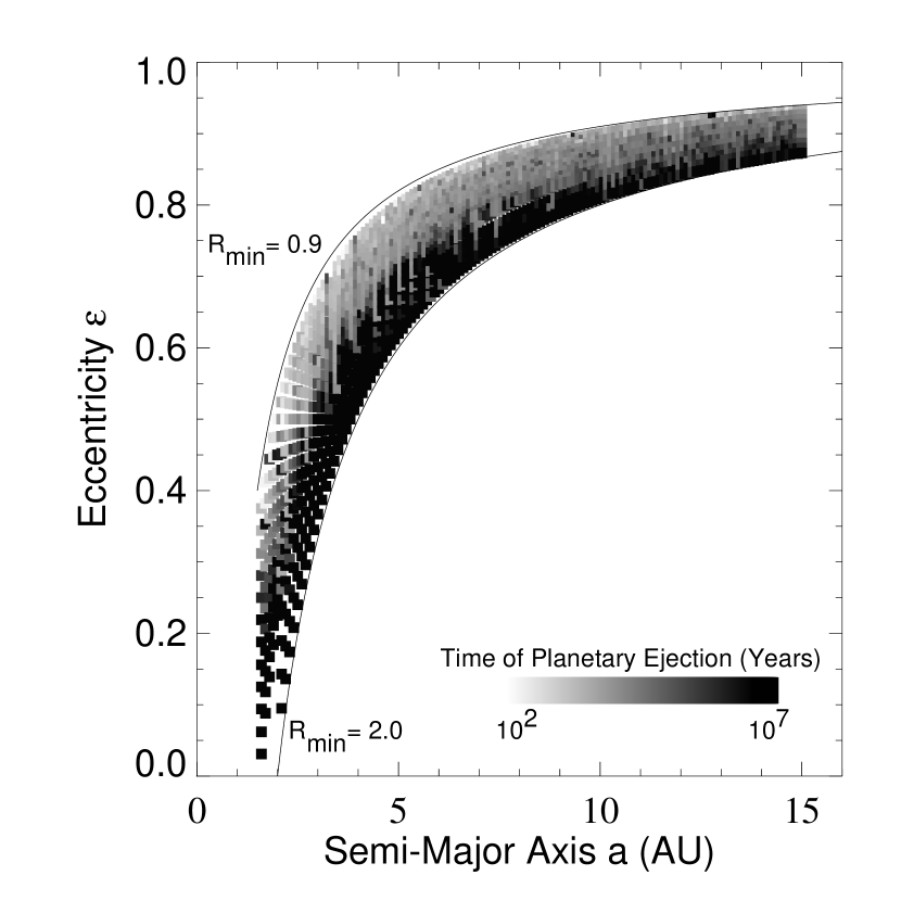
Figure 3: Results of numerical simulations for $M_{C}=0.001M_{\odot}$. Top panel shows the gray scale plot of survival time as a function of the location in the $a-\epsilon$ plane (using results from the symplectic code). The lower panel shows the empirical form for the survival time as a function of periastron distance ${R_{\rm min}}$. The starred symbols show the results from the symplectic code, whereas the filled triangles show the results from the B-S code (the triangles are slightly offset for clarity).

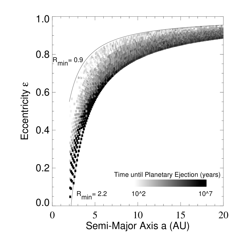
Figure 4: Results of numerical simulations for $M_{C}=0.01M_{\odot}$. Top panel shows the gray scale plot of survival time as a function of the location in the $a-\epsilon$ plane (using results from the symplectic code). The lower panel shows the empirical form for the survival time as a function of periastron distance ${R_{\rm min}}$.The starred symbols show the results from the symplectic code, whereas the filled triangles show the results from the B-S code (the triangles are slightly offset for clarity).

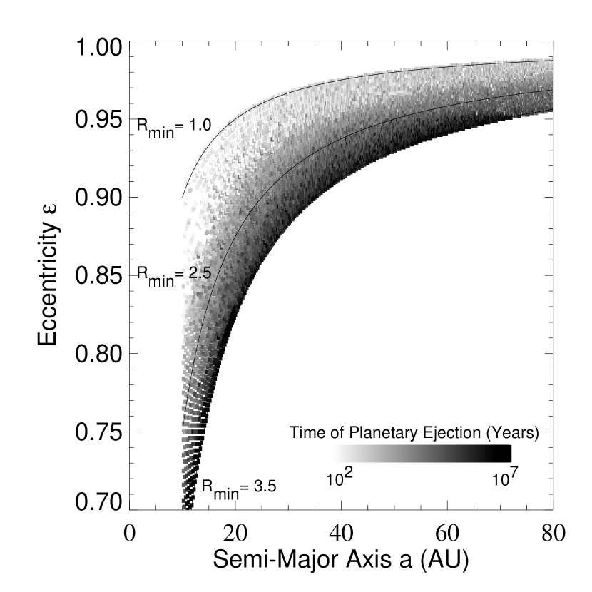
Figure 5: Results of numerical simulations for $M_{C}=0.1M_{\odot}$. Top panel shows the gray scale plot of survival time as a function of the location in the $a-\epsilon$ plane (using results from the symplectic code). The lower panel shows the empirical form for the survival time as a function of periastron distance ${R_{\rm min}}$. Only the top part of the plane ($\epsilon\geq 0.7$) is shown in the upper panel, but the full range of $\epsilon$ was sampled to obtain the slope of fitted line depicted in the lower panel. The starred symbols show the results from the symplectic code, whereas the filled triangles show the results from the B-S code (the triangles are slightly offset for clarity).

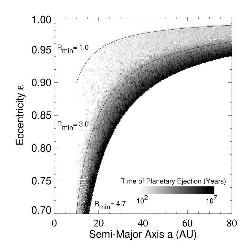
Figure 6: Results of numerical simulations for $M_{C}=0.5M_{\odot}$. Top panel shows the gray scale plot of survival time as a function of the location in the $a-\epsilon$ plane (using results from the symplectic code). The lower panel shows the empirical form for the survival time as a function of periastron distance ${R_{\rm min}}$. Only the top part of the plane ($\epsilon\geq 0.7$) is shown in the upper panel, but the full range of $\epsilon$ was sampled to obtain the slope of fitted line depicted in the lower panel. The starred symbols show the results from the symplectic code, whereas the filled triangles show the results from the B-S code (the triangles are slightly offset for clarity).

Using the symplectic integration scheme, we have performed an ensemble of approximately 35,000 simulations of the Sun-Earth-companion system. The semi-major axis of the companion is chosen to vary in even increments from 1 AU (where Earth is ejected almost immediately) out to 15 AU (for the 1 $m_{J}$ companion), 20 AU (for the 10 $m_{J}$ companion), and 80 AU (for the 0.1 and 0.5 $M_{\odot}$ stellar mass companions). For each choice of semi-major axis, the eccentricity is chosen to sample a range of periastron values from ${R_{\rm min}}$ = 1 AU out to values so large that the ejection time always exceeds the 10 Myr range of our integrations. For each choice of companion mass, eccentricity, and semi-major axis, the remaining phase angles are chosen from a random distribution. This sampling of parameter space fills a broad band in the $a-\epsilon$ plane, as shown by the gray scale plots in Figures 3 – 6. For the portion of the $a-\epsilon$ plane to the upper left of the chosen region, the companion crosses the Earth orbit and would lead to rapid ejection. For the portion of the $a-\epsilon$ plane to the lower right of the sampled region, the ejection times are longer than 10 Myr.

The results obtained using the symplectic code are presented by ascending order of companion mass in Figures 3 – 6. The top panel of each figure depicts a grayscale plot of ejection times in the $a-\epsilon$ plane, where the darker shades correspond to longer ejection times. Contour lines of constant periastron ${R_{\rm min}}=a(1-\epsilon)$ are included for reference. A natural dependency of the ejection time on ${R_{\rm min}}$ is clearly illustrated by the grayscale plots, with the largest gradients occurring perpendicular to contour lines. To elucidate this trend, we plot the ejection time versus ${R_{\rm min}}$ for each companion mass in the corresponding lower panel. Although the ejection time depends most sensitively on the periastron value, the relevant initial conditions that describe the binary continue to be the eccentricity and semi-major axis. In the Figures, the star symbols represent the average value of $\log{\tau_{\rm ej}}$ (for each given value of ${R_{\rm min}}$) and the vertical bars represent one standard deviation about the mean. The width of the distribution (at constant periastron) arises from two sources: (A) For a given type of binary (i.e., given $\epsilon$ and $a$), the ejection time has a distribution of values as shown in Figure 1. (B) For binaries with differing values of $(a,\epsilon)$, but constant periastron ${R_{\rm min}}=a(1-\epsilon)$, the ejection time has additional variation (e.g., see HW99). Although the ejection times vary by an order of magnitude at a given value of ${R_{\rm min}}$, a clear functional dependence for the mean value can nonetheless be extracted from the results. Over the sampled range of periastron values ${R_{\rm min}}$, the mean ejection time follows a straight line in the semi-log plots. In the following section, we will use this property to extrapolate our results out to longer ejection time scales.

We note that the importance of the periastron distance has been found in related dynamical investigations. In a study of scattering of Trans-Neptunian objects by the planet Neptune (Holman, Grav, & Gladman 2001), the borders of the region where the bodies become chaotic are approximately described by lines of constant perihelia (that study also discusses the departures from this trend). In a related work (Duncan, Levison, & Budd 1995), objects with perihelia less than about 35 AU were found to be unstable, apparently due to cumulative effects of random forces from Neptune (exerted near perihelion). Finally, the ejection time in systems of terrestrial planets can be modeled with an equation similar to our equation [4] (see Chambers, Wetherill, & Boss 1996).

In an alternate set of simulations, we have performed an ensemble of approximately 8000 numerical integrations using the B-S code. The results from the sympletic code suggested that the periastron is the most important variable for determining the ejection time. For the B-S integrations, we chose even increments in periastron ${R_{\rm min}}$ of the companion. For each value of ${R_{\rm min}}$, we sample the eccentricity over the full range $0\leq\epsilon\leq 1$ and perform multiple realizations of the experiments using different (random) choices for the remaining phase angles. This coverage of parameter space is complementary to that used for the symplectic code. The symplectic code was used to sample as much of the $a-\epsilon$ plane as possible. The B-S code was used to sample fewer values of $(a,\epsilon)$, and fewer values of the periastron, but each point in the $a-\epsilon$ plane was studied with more realizations of the various phase angles in the problem. The ejection time, as a function of periastron, follows the same general trend for both ensembles of numerical experiments, as shown in the bottom panels of Figures 3 – 6 (where results from the B-S code are plotted as triangular symbols). The main difference between the two explorations of parameter space is that the latter displays a somewhat wider distribution of ejection times for a given periastron value. However, the expectation values of the distributions are in good agreement.

To package these results in a useful format, we fit the numerically determined mean ejection times with an empirical relation of the form

$${\tau_{\rm ej}}={\tau_{\rm ej}}_{0}\exp\Bigl{[}\alpha(p-1)\Bigr{]}\,,$$ (4)

where ${\tau_{\rm ej}}_{0}$ is a fiducial time scale, $p$ is the dimensionless periastron distance $p\equiv({R_{\rm min}}$/1 AU), and $\alpha$ is the dimensionless fitting parameter (the slope of the lines in Figures 3 – 6). The variables for the functional fits are presented in Table 1 below, for the four companion masses $M_{C}$ considered here. The Table also lists the range in ${R_{\rm min}}$ over which the fitting formulae have been numerically determined. For the stellar mass companions, the ejection time is extremely short (hundreds of years) for a small range of periastron near 1 AU; the fit to equation [4] thus begins at larger periastron values.

Table 1: Parameters for ejection time scaling laws

mass $M_{C}$ ($M_{\odot}$)	${\tau_{\rm ej}}_{0}$ (yr)	$\alpha$	periastron range
0.001	1800	9.8 $\pm$ 3.0	1 AU $<{R_{\rm min}}<$ 1.8 AU
0.01	400	6.8 $\pm$ 1.1	1 AU $<{R_{\rm min}}<$ 2.1 AU
0.10	110	4.1 $\pm$ 0.67	1.6 AU $<{R_{\rm min}}<$ 3.5 AU
0.50	0.64	4.7 $\pm$ 0.32	2.4 AU $<{R_{\rm min}}<$ 4.4 AU

Although the ejection time depends most sensitively on the variable ${R_{\rm min}}$, this time scale ${\tau_{\rm ej}}$ is basically a function of $a$ and $\epsilon$. Close inspection of Figures 3 – 6 shows that nearby points in the $a-\epsilon$ plane can lead to rather different ejection times. In addition, systems with the same values of $a$ and $\epsilon$ can display differing ejection times for varying starting phases of the orbiting bodies – as illustrated in Figure 1. These systems are thus chaotic, in the technical sense, and display sensitive dependence on their initial conditions. This variation leads to a range of values for ${\tau_{\rm ej}}$, as quantified by the error bars in the lower panels of Figures 3 – 6. For a given value of ${R_{\rm min}}$, the ejection time ${\tau_{\rm ej}}$ displays a full distribution of values. As mentioned earlier, the width of this distribution arises from two sources. First, the distribution of ejection times has an intrinsic spread for a given pair $(a,\epsilon)$, as shown in Figure 1. Second, we are averaging over many pairs $(a,\epsilon)$ with the same periastron; since the ejection time can depend on both $a$ and $\epsilon$ (e.g., HW99), this averaging increases the width of the distribution as shown by the error bars in the lower panels of Figures 3 – 6. The fitting formulae found above (see Table 1) provide an estimate for the expectation value of this distribution as a function of ${R_{\rm min}}$ (where the expectation value is the mean value, averaged over the underlying probability distribution of ejection times).

The results shown in Figures 3 – 6 are in basic agreement with previous work. In a study of Alpha Centauri, test particles were found to be stable for initially circular orbits within about 3 AU of either star (Wiegert & Holman 1997), where the integration time was 32,000 binary periods. In this binary, the mass ratio is close to 0.5, the periastron distance is 11.2 AU, and the semi-major axis is 23 AU. Scaled to the units of this paper, the boundary of stability corresponds to a time scale of $\tau\approx 4.8\times 10^{5}$ yr for $p\approx 3.7$. This point falls just above the best fit line shown in the bottom panel of Figure 6, but well within the allowed range. In a more general study, HW99 found the critical radius $a_{cr}$ for which a planet will remain stable for $10^{4}$ binary periods. For a given binary mass ratio, the critical radius is a function of eccentricity (see Table 3 of HW99). When scaled to the Sun-Earth-companion systems considered here (with one year planetary orbits), the function $a_{cr}(\epsilon)$ can be converted to a function ${\tau_{\rm ej}}(p)$, where ${\tau_{\rm ej}}$ corresponds to $10^{4}$ binary orbits. The resulting function ${\tau_{\rm ej}}(p)$ includes only one eccentricity value for a given value of $p$, rather than an average over a path in the $a-\epsilon$ plane as we use here. Nonetheless, the RMS value of the relative difference (in $\log\tau$) between the HW99 result and that predicted by equation [4] is only about 7% for a companion mass $M_{C}$ = 0.1 $M_{\odot}$ and 12% for $M_{C}$ = 0.5 $M_{\odot}$.

The results from our lowest companion mass simulations were confirmed for a limited number of cases using the MERCURY integration package (Chambers 1999). For systems with a Jupiter-mass companion, integrations were performed for periastron ${R_{\rm min}}$ ranging from 1.04 – 2.60 AU. For some of these simulations, the companion began in the same orbital plane as the Sun-Earth system (as before). We also ran an alternate series of simulations in which Jupiter began with an inclination of 1.3^∘ relative to the Sun-Earth orbital plane; for comparison purposes, identical sets of simulations were also performed treating the Earth as a mass-less test particle. In all of the simulations, the other orbital elements were chosen at random. Each system’s evolution was then followed for 100 Myrs or until the Earth was lost from the system.

For simulations with a starting inclination angle for Jupiter, the results for periastron ${R_{\rm min}}$ = 1.04 AU show an interesting departure from the co-planar simulations. These simulations (where Jupiter starts with $i$ = 1.3^∘) display a wider range of ejection times, but the average value remains essentially the same. Although the orbit of the companion brings it alarmingly close to Earth’s orbit, some of the simulations show relatively long ejection times. For example, in a simulation with Jupiter’s ${R_{\rm min}}$ = 1.04 AU and $\epsilon$=0.83, after 20,000 years, the (massive) Earth has been perturbed into an orbit with $a$ = 9.2 AU, $\epsilon$ = 0.6, and an inclination of $i$ = 139^∘. The Earth’s eccentricity and inclination continue to oscillate for several hundred thousand years until the Earth is ejected from the system.

The MERCURY results verify that the range 1.6 AU $<{R_{\rm min}}<$ 1.8 AU marks the transition between instability and stability. Most of the systems with ${R_{\rm min}}<$ 1.7 AU lose the Earth in less than 10 Myr, whereas systems with ${R_{\rm min}}>$ 1.9 AU remain stable for 100 Myr. The stability of the high ${R_{\rm min}}$ systems was examined further through a series of 500 Myr runs using ${R_{\rm min}}$ = 1.87 – 2.01 AU and Jupiter’s eccentricity $\epsilon_{J}$ = 0.1 – 0.8. Many of the systems remained stable for the duration of the integration, although there were several exceptions: With ${R_{\rm min}}$ = 1.87 and $\epsilon$=0.1, for example, the Earth was ejected from the system in only 0.3 Myr. However, the other systems with $\epsilon$ = 0.1 and ${R_{\rm min}}>1.87$ remained stable for the full 500 Myr, as did the systems with 0.1 $\leq\epsilon\leq$ 0.7. On the other hand, half of the systems with $\epsilon$ = 0.8 became unstable, with Earth being ejected from the system or accreted by the star. Taken together, these results are consistent with the ejection times predicted by the fit of equation [4], although the ejection time may be even longer (at large values of periastron) than that predicted by the fitting function. A larger ensemble of long term integrations is needed to clarify this issue. One should also keep in mind that equation [4] represents the expectation value of the distribution; for a given value of ${R_{\rm min}}$, the distribution has a width of nearly an order of magnitude in ejection time ${\tau_{\rm ej}}$.

4 Fraction of binary systems that allow Earths

This set of numerical experiemnts can be used to address the question of habitable planets. Although habitability includes many aspects, a key requirement is for the planet to remain stable over long time intervals. The majority of stars reside in binary systems and these companions can preclude the possibility of an Earth-like planet, i.e., a small planet in a 1 AU (nearly circular and stable) orbit about a solar type star. The results of the previous section indicate that the survival time of such an Earth increases with the periastron distance ${R_{\rm min}}$. In this section, we extrapolate our numerical results to longer times and find an approximate lower bound on the fraction of binary star systems that allow for habitable planets.

The numerical results of the previous sections are complete out to ejection times of 10 million years and include limited results out to 500 million years. Although the time required for life to develop on a planet is largely unknown, the most familiar habitable planet – our Earth – has an age of 4.6 Gyr. Since we want to find a conservative estimate for the fraction of binary systems that allow for habitability, we assume that an Earth-like planet must remain stable for 4.6 Gyr.

The ejection times for a given value of ${R_{\rm min}}$ span a wide range, as shown in Figures 3 – 6. Again adopting a conservative approach, we assume that the ejection times take the shortest values within their allowed range, and hence the ejection times are about 10 times shorter than the numerically determined expectation values (as fit by equation [4]). Our estimate for the minimum periastron distance required for survival over a time $\tau_{SS}$ thus takes the form

$$p>1+\alpha^{-1}\ln[10\tau_{SS}/{\tau_{\rm ej}}_{0}]\,,$$ (5)

where $p$ is the periastron ${R_{\rm min}}$ in units of AU. For the sake of definiteness, we take $\tau_{SS}$ = 4.6 Gyr, the current age of the solar system. In adopting the form [5], we are assuming that equation [4] continues to hold out to larger periastron values and longer ejection times. Since our (limited) longer term integrations indicate that Earth-like planets may survive even longer than predicted by an extrapolation of equation [4], the limit implied by equation [5] represents a conservative bound. The parameters ${\tau_{\rm ej}}_{0}$ and $\alpha$ are given in Table 1 for companions of various masses.

We note that this constraint can be generalized. If we consider an Earth-like planet with circular orbit of radius ${\tilde{a}}$ = $a$/(1AU) in orbit about a primary star of mass $m=M_{\ast}/(1M_{\odot})$, and we want to enforce stability for a time $\tau$, the required constraint becomes

$$p>{\tilde{a}}\Bigl{\{}1+\alpha^{-1}\ln[(10\tau/{\tau_{\rm ej}}_{0})m^{1/2}{\tilde{a}}^{-3/2}]\Bigr{\}}\,.$$ (6)

The values of $\alpha$ and ${\tau_{\rm ej}}_{0}$, as listed in Table 1, apply to rescaled companion masses $\widetilde{M}_{C}$ = $mM_{C}$ (where $M_{C}$ are the masses given in the table).

Now we specialize back to our standard case of a 1.0 $M_{\odot}$ primary and an initial Earth orbit of 1 AU. For companion masses $M_{C}$ = 0.1 and 0.5 $M_{\odot}$, the minimum value of the periastron distance required for stability (according to equation [5]) is about $p=6-7$, as derived from the range of allowed slopes listed in Table 1. To be conservative, once again, we use the high end of this estimated range. To find a lower limit on the fraction of binaries that allow for habitable Earths, we thus need to find the fraction of binary systems with dimensionless periastron $p>7$.

The observed population of binaries has a well-defined period distribution (DM91), which takes a log-normal form. Focusing on the case of primary stars with masses of approximately 1.0 $M_{\odot}$, we can convert the period distribution into the probability distribution for semi-major axes $a$. The resulting normalized distribution thus takes the form

$$dP_{a}=f(\ln a)d\ln a\,=\,{1\over\sqrt{2\pi}\,\,\sigma}\,\exp\Bigl{[}-{(x-x_{0})^{2}\over 2\sigma^{2}}\Bigr{]}\,dx\,,$$ (7)

where the variable $x$ is the logarithm of the dimensionless semi-major axis. The parameters $x_{0}$ and $\sigma$ are determined from fits to the observed binary period distribution (as reported in DM91). The dimensionless width $\sigma$ = 3.53. To convert the period distribution to a distribution of semi-major axis, we must include the ratio $\mu$ of the companion mass to the primary mass through the relation $x_{0}$ = 3.44 $+(1/3)\ln[1+\mu]$. As a result, the distribution depends (weakly) on the value of the mass ratio $\mu$.

The distribution of eccentricity is also well defined, but the observed distribution takes a different form for close, intermediate, and wider binaries (DM91). In the present context, we are interested in binaries with periastron distances greater than about 7 AU, so the semi-major axes are also greater than 7 AU and we can use the eccentricity distribution for wider binaries. In this regime, the eccentricity distribution has the simple form $dP_{\epsilon}=2\epsilon d\epsilon$ (DM91). Furthermore, for these wider binaries, the eccentricity is independent of semi-major axis (DM91, Heacox 1998).

For a given mass ratio $\mu$, we define $F_{\mu}(p)$ to be the fraction of binary systems with dimensionless periastron greater than $p$. To evaluate $F_{\mu}(p)$, we must integrate over the portion of the $a-\epsilon$ plane with periastron $a(1-\epsilon)>p$, where the integrand is weighted by both the eccentricity distribution and the distribution of semi-major axes (described above). The eccentricity integration can be done analytically and the remaining integral – which defines the fraction $F_{\mu}(p)$ as a function of $p$ – takes the form

$$F_{\mu}(p)={1\over\sqrt{2\pi}\,\,\sigma}\int_{\ln p}^{\infty}dx\bigl{(}1-p{\rm e}^{-x}\bigr{)}^{2}\exp[-(x-x_{0})^{2}/2\sigma^{2}]\,.$$ (8)

The fraction $F_{\mu}(p)$ is a slowly varying function of the mass ratio $\mu$. To estimate the fraction $F(p)$ of all binary systems for which Earth-like planets can remain stable, we must find the weighted average of $F_{\mu}(p)$, i.e.,

$$F(p)\equiv\int_{0}^{1}w(\mu)F_{\mu}(p)d\mu\,,$$ (9)

where the distribution of mass ratios $dP_{\mu}=w(\mu)d\mu$. This distribution has been observed and is presented in DM91 (see Table 7 and Figure 10). The peak of the distribution occurs near $\mu$ = 0.3 and the majority of systems have mass ratios in the range $0.1\leq\mu\leq 0.5$. We use DM91 to specify the distribution $w(\mu)$ of mass ratios and evaluate the integral of equation [9]. The resulting function $F(p)$ is shown in Figure 7.

Figure 7 also shows a fit to the numerically determined result. The fitting function is chosen to have the simple form

$${\widetilde{F}}(p)=F_{1}\exp\bigl{[}-(a\xi+b\xi^{2})\bigr{]}\,,$$ (10)

where $F_{1}$ = 0.711, $a$ = 0.101, $b$ = 0.0287, and $\xi=\ln[p]$. The function [10] provides a good approximation to the numerically determined result, with an absolute error less than about 0.011 and a relative error less than 4 percent. More exact fits are not warranted, as the observed distributions of binary orbital parameters are not known to this accuracy. This function can be used to estimate the fraction of binary systems with periastron greater than any specified value within the allowed range $1<p<10^{5}$.

As argued above, stability of Earth over 4.6 Gyr requires a stellar companion to have $p>7$ (${R_{\rm min}}>7$ AU), where this value has been estimated from numerical experiments using companion masses in the range $M_{C}=0.1-0.5M_{\odot}$ (which are typical values – see DM91). The fraction of binary systems that meet this constraint and allow habitable Earth-like planets is 0.5 (or 50 percent). This estimate should be regarded as a lower bound on the fraction. Additional binary systems could allow for habitable Earths if the orbits can be inclined. Notice also that this estimate does not include close binary systems, those with separations $a\ll 1$ AU. Although sufficiently close binary systems could allow Earth to remain stable (see, e.g., HW99), the companion will necessarily reside within 1 AU of the Earth and the companion’s radiative flux could affect considerations of habitability. For the wider binaries considered here, the requirement of dynamical stability demands that ${R_{\rm min}}>7$ AU so that the companion is always farther than about 6 AU from Earth. The additional radiative flux of the secondary is always less than about 3% of that of the primary. For a more typical companion mass, say $M_{C}=0.4M_{\odot}$, the flux from the secondary is less than 0.2% of the total.

The numerical results of the previous section show that Sun-Earth-companion systems can remain stable for relatively long times – such as the current 4.6 Gyr age of our solar system – even though they do not meet the analytic criteria for stability (see equations [1–3]). To illustrate this point, Figure 8 shows the allowed region of the $a-\epsilon$ plane for Earth-like planets in binary systems. The solid curves delineate the region of the plane that allows Earth to remain stable for 4.6 Gyr, as estimated here, whereas the dashed curves delineate the (much smaller) region of the plane for which the system is Hill stable. The allowed region is that below each curve. Figure 8 emphasizes that the requirement of system stability over geological, biological, and even cosmological time scales (equations [5, 6]) can be less restrictive and more relevant than the requirement of Hill stability (equation [2]).

5 Conclusion

This paper presents numerical simulations of Earth-like planets in binary systems. These binaries have solar mass primaries and companion masses in the range 0.001 $M_{\odot}$ (Jovian mass) to 0.5 $M_{\odot}$ (K stars), although the results can be scaled to other choices. The first result of this work is an estimate of the ejection times for Earth-like planets in these systems (Figs. 3 – 6). For a given companion mass, the ejection time depends most sensitively on the periastron distance ${R_{\rm min}}$. Although the ejection time shows a wide range for a given value of ${R_{\rm min}}$, the overall trend is well-defined and the expectation value of the distribution can be described by an exponential function of ${R_{\rm min}}$. We have fit our numerical results, for each companion mass, to find the mean ejection time as a function of periastron (see equation [4] and Table 1).

The second result of this work is an estimate for the fraction of binary systems with Sun-like primaries that allow an Earth-like planet to remain stable for a specified time period. Our numerical experiments suggest that the requirement for stability can be written in terms of a minimum periastron distance for the binary orbit. The resulting constraint is provided by equations [5 – 6] (where the fitting parameters $\alpha$ and ${\tau_{\rm ej}}_{0}$ have been calculated for companion masses $M_{C}$ = 0.001 – 0.5 $M_{\odot}$). For the observed distributions of binary orbital parameters (DM91), the fraction of binaries that have periastron distances greater than a given value is specified by equations [9 – 10] and Figure 7. Taken together, these results imply that at least 50 percent of the binary systems allow an Earth-like planet to remain stable for 4.6 Gyr (the current age of the solar system). Because the ejection time is a much more sensitive function of periastron than the fraction of binary systems (with periastron greater than a given value), this estimate is quite robust; for example, if we were to adopt the overly conservative stability requirement that ${R_{\rm min}}>20$ AU, the fraction of viable binary systems would still be 40 percent. We also note that the condition of system stability over billions of years is much less restrictive than the requirement of Hill stability (see Figure 8).

This type of stability analysis can be applied to the observed planetary systems now being discovered in association with nearby stars (e.g., Mayor & Queloz 1995; Butler et al. 1999, Marcy et al. 2001, Fischer et al. 2002). For a subset of the known extrasolar planetary systems, those with $a>1.5$ AU, we have performed additional sets of numerical simulations using the masses and orbital properties of the observed giant planets as the companions. An Earth-like planet, with the mass of Earth and an orbital radius of 1 AU, is assumed to reside in each system; we then study its intermediate term prospects for stability. Figure 9 shows the result – the estimated ejection time for Earth-like planets plotted as a function of the observed periastron distance of the giant planet. Each system displays a range of ejection times for the hypothetical Earth (the vertical bars in the Figure show the standard deviation of this distribution). The systems with periastron greater than about 1.8 AU allow an Earth-like planet to survive for more than 10 Myr. Extrapolating this result to the age of the galaxy, about 10 Gyr, we estimate that systems with Jupiter mass companions and periastron greater than 2.8 AU would remain stable; for companions with 10 Jupiter masses, the minimum periastron distance is about 4 AU.

The parameter space available to this class of systems is enormous and additional numerical work should be carried out. This paper provides an exploration of the $a-\epsilon$ plane using integration times out to 10 Myr, but longer term simulations should be done for $t\gg 10$ Myr. In the regime studied here, the ejection time varies according to the exponential law of equation [4]. At sufficiently large value of periastron, however, chaotic motion should no longer occur and the system should become stable. In addition, this work focuses on co-planar orbits, although longer ejection times can be realized for varying orbital inclinations. This work also studies only single planets, whereas multiple planets systems can also be considered. Under favorable circumstances, multiple planets can protect each other from ejection (M. Holman, private communication); if the orbital precession induced by the other planets occurs on a shorter time scale than that induced by the binary companion, the perturbations of the companion can be washed out. This work only considers the stability of Earth-like planets with outer binaries, where the Earth lies within the orbit of the secondary; the case of inner binaries, with Earth orbiting the binary pair, should also be investigated. Finally, this paper studies the stability of three-body systems after the Earth-like planet has formed. The presence of a binary companion can affect the planetary formation process, and an investigation of this issue is underway (Quintana 2003).

Acknowledgements

This study began as an REU project for EMD at the University of Michigan. We would like to thank Matt Holman and Greg Laughlin for useful discussions and an anonymous referee for many useful comments that improved the paper. EMD and MF are supported by the Hauck Foundation through Xavier University. EVQ and FCA are supported by NASA through a grant from the Origins of Solar Systems Program and by the University of Michigan through the Michigan Center for Theoretical Physics.

Figure 1: The distribution of ejection times for different realizations of the same system. In this set of the experiments, the binary companion has mass $M_{C}$ = 0.1 $M_{\odot}$, eccentricity $\epsilon$ = 0.5, and semi-major axis $a$ = 5 AU. The solid histogram shows the distribution of ejection times resulting from the B-S code (for a random sampling of the starting phase angles). The dashed histogram shows the corresponding distribution of ejection times resulting from the symplectic code (again, for a random sampling of phase angles). The smooth curve shows a log-normal distribution with the same peak value and width as the computed distributions. Notice that the distributions predicted by both numerical codes are similar and that both have a log-normal form (with the same width and peak location).

Figure 2: The distribution of eccentricity for the Earth-like planet for different epochs of a single numerical integration. In this experiment, the binary companion has mass $M_{C}$ = 0.1 $M_{\odot}$, eccentricity $\epsilon$ = 0.5, and semi-major axis $a$ = 5 AU. The dotted histogram on the left shows the distribution of eccentricity over the first $10^{4}$ yr of the integration. The next three histograms show the eccentricity distribution over $10^{4}$ yr intervals starting at $5\times 10^{4}$ yr (dashed curve), $8\times 10^{4}$ yr (dot-dashed curve), and the final interval ending at $\sim 10^{5}$ yr (solid curve). The eccentricity of the Earth-like planet thus displays a distribution of values, and this distribution evolves toward higher eccentricity values with time.

Figure 7: Fraction of binary systems that have dimensionless periastron distances greater than $p$, plotted as a function of $p$ = $a(1-\epsilon)$/(1AU). This fraction is determined from the observed distributions of binary periods and orbital eccentricities (as reported in DM91). The dashed curve shows an analytic fit to the numerical result (see equation [10]). The numerical simulations depicted in the previous figures indicate that the minimum periastron required for Earth to survive 4.6 Gyr is about 7 AU. This constraint, in conjunction with the distribution shown above, indicates that more than 50 percent of binary systems allow for habitable Earths.

Figure 8: Comparison of analytic and numerical constraints on survival time for Earth-like planets in binary systems with Sun-like primaries. The solid curves show the portion of the $a-\epsilon$ plane that allow for Earth-like planets to remain stable over the current age of the solar system. The allowed region of the plane falls below the curves, which are displayed for companion masses $M_{C}$ = 0.001 $M_{\odot}$ (top), 0.01 $M_{\odot}$, 0.1 $M_{\odot}$, and 0.5 $M_{\odot}$ (bottom). The dashed curves show the analytic constraints (eqs. [1 – 3]) that require the system to be stable according to the Hill condition. Again, the allowed region falls below the curves, which are shown for companion masses $M_{C}$ = 0.001 $M_{\odot}$ (top), 0.01 $M_{\odot}$, 0.1 $M_{\odot}$, and 0.5 $M_{\odot}$ (bottom). Hill stability implies a much stronger constraint than the requirement that Earth has a stable orbit for 4.6 Gyr.

Figure 9: Results of numerical simulations for known extrasolar planetary systems. The estimated survival time for Earth-like planets is plotted as a function of the observed periastron distance of the secondary (the extrasolar giant planet). The size of the plotting symbols is proportional to the logarithm of the planet mass. The vertical bars on each planetary symbol show the standard deviation for the distribution of ejection times for the hypothetical Earth in the system. The solid curve shows the expectation value of the ejection time for a planetary companion with mass $M_{C}=0.001M_{\odot}$; the dashed curve shows the expectation value for $M_{C}=0.01M_{\odot}$.

References

- (1) Abt, H. 1983, ARA&A, 21, 343
- (2) Adams, F. C., & Laughlin, G. 2003, Icarus, in press, astro-ph/0301561
- (3) Benest, D. 1996, A&A, 314, 983
- (4) Butler, R. P., et al. 1999, ApJ, 526, 916
- (5) Chambers, J. E. 1999, MNRAS, 304, 793
- c (2) Chambers, J. E., Wetherill, G. W., & Boss, A. P. 1996, Icarus, 119, 261
- (7) Duncan, M. J., Levison, H. F., & Budd, S. M. 1995, AJ, 110, 3073
- (8) Duncan, M. J., & Lissauer, J. J. 1998, Icarus, 134, 303
- Duquennoy and Mayor (1991) Duquennoy, A., & Mayor, M. 1991, A&A 248, 485 (DM91)
- (10) Dvorak, R., Pilat-Lohinger, E., Funk, B., & Freistetter, F. 2003, A&A, 398, L1
- (11) Fischer, D. A., et al. 2002, ApJ, 564, 1028
- (12) Gehman, C. S., Adams, F. C., & Laughlin, G. 1996, PASP, 108, 1018
- (13) Ghez, A. M., Neugebauer, G., & Matthews, K. 1993, AJ, 106, 2005
- (14) Gladman, B. 1993, Icarus, 106, 247
- (15) Heacox, W. D. 1998, AJ, 115, 325
- (16) Holman, M., Grav., T., & Gladman, B. 2001, DDA, 32, 1102
- (17) Holman, M. J., & Wiegert, P. A. 1999, AJ, 117, 621 (HW99)
- (18) Kasting, J. F., Whitmire, D. P., & Reynolds, R. T. 1993, Icarus, 101, 108
- (19) Laughlin, G., & Adams, F. C. 1999, ApJ, 526, 881
- (20) Laughlin, G., & Adams, F. C. 2000, Icarus, 145, 614
- (21) Laughlin, G., Chambers, J., & Fischer, D. 2002, ApJ, 579, 455
- (22) Lecar, M., Franklin, F. A., & Holman, M. J. 2001, ARA&A, 39, 581
- le (0) Lecar, M., Franklin, F., & Murison, M. 1992, AJ, 104, 1230
- (24) Levison, H. F., Lissauer, J. J., & Duncan, M. J. 1998, AJ, 116, 1998
- (25) Lissauer, J. J. 1993, ARA&A, 31, 129
- (26) Marcy, G. W., et al. 2001, ApJ, 556, 296
- (27) Mayor, M., & Queloz, D. 1995, Nature, 378, 355
- (28) Menou, K., & Tabachnik, S. 2003, ApJ, 583, 473
- (29) Milani, A., & Nobili, A. M. 1983, Celest. Mech., 31, 213
- (30) Murray, C. D., & Dermott, S. F. 2000, Solar System Dynamics (Cambridge: Cambridge Univ. Press)
- (31) Press, W. H., et al. 1992, Numerical Recipes: The art of scientific computing (Cambridge: Cambridge Univ. Press)
- (32) Quintana, E. V. 2003, PhD Thesis, University of Michigan
- (33) Rabl, G., & Dvorak, R. 1988, A&A, 191, 385
- (34) Rampino, M. R., & Caldeira, K. 1994, ARA&A, 32, 83
- (35) Rivera, E. J., & Lissauer, J. J. 2000, ApJ, 530, 454
- (36) Rivera, E. J., & Haghighipour, N. 2003, ASP Conference Series, Vol. 294, 205
- (37) Ruden, S. P. 1999, in Origin of Stars and Planetary Systems, eds. C. J. Lada & N. D. Kylafis (Kluwer Academic Publishers), p. 643
- (38) Szebehely, V. 1980, Celest. Mech., 22, 7
- (39) Tinney, C. G., et al. 2002, ApJ, 571, 528
- (40) Valsecchi, G. B., Carusi, A., & Roy, A. 1984, Celest. Mech., 32, 217
- (41) Wiegert, P. A., & Holman, M. J. 1997, AJ, 113, 1445
- (42) Wisdom, J., & Holman, M. 1991, AJ, 102, 1528