Optimal Weak Lensing Skewness Measurements

Abstract

Weak lensing measurements are starting to provide statistical maps of the distribution of matter in the universe that are increasingly precise and complementary to cosmic microwave background maps. The most common measurement is the correlation in alignments of background galaxies which can be used to infer the variance of the projected surface density of matter. This measurement of the fluctuations is insensitive to the total mass content and is analogous to using waves on the ocean to measure its depths. However, when the depth is shallow as happens near a beach waves become skewed. Similarly, a measurement of skewness in the projected matter distribution directly measures the total matter content of the universe. While skewness has already been convincingly detected, its constraint on cosmology is still weak. We address optimal analyses for the CFHT Legacy Survey in the presence of noise. We show that a compensated Gaussian filter with a width of 2.5 arc minutes optimizes the cosmological constraint, yielding $\Delta\Omega_{m}/\Omega_{m}\sim 10\%$. This is significantly better than other filters which have been considered in the literature. This can be further improved with tomography and other sophisticated analyses.

1 Introduction

Mapping the mass distribution of matter in the Universe has been a major challenge and focus of modern observational cosmology. The only direct procedure to weigh the matter in the universe is by using the deflection of light by gravity. While this effect is very small, a large statistical sample can provide a precise measurement of averaged quantities.

There are very few direct ways to weigh the universe. The most accurate measurement by combining CMB data with large scale structure (Spergel et al., 2003; Contaldi et al., 2003) results in $\Omega_{m}\sim 0.27$ with zero geometric curvature implying a cosmological constant $\Omega_{\Lambda}\sim 0.73$. This type of inference requires combining data measured at different times and on different length scales. Blanchard et al. (2003) have shown that the same data can be consistent with $\Omega_{m}=1$ if one gives up perfect scale invariance for the primordial perturbations and allows for a neutrino mass of 1eV. The physical constraint arises since the CMB measures the fluctuations on large scales $L\sim$Gpc at high redshift $z\sim 1100$. The large-scale structure measures scales of $L\sim 1-100$ Mpc and a low redshift of $z\sim 0$. The scales only have a small overlap (Tegmark & Zaldarriaga, 2002). If one requires perfect scale invariance of the fluctuations, one is forced into a low matter density with a cosmological constant. It is perhaps an aesthetic choice to trade scale invariance in time to scale invariance in space.

Weak gravitational lensing provides a direct statistical measure of the dark matter distribution regardless of the nature and dynamics of both the dark and luminous matter intervening between the distant sources and observer. Weak lensing by large-scale structure can lead to the shear and magnification of the images of distant faint galaxies. Based on the theoretical work done by Gunn (1967), Blandford et al. (1991), Miralda-Escude (1991) and Kaiser (1992) performed the first calculation of weak lensing by large-scale structure, the result of which showed the expected distortion amplitude of weak lensing effect is at a level of roughly a few percent in adiabatic cold dark matter models. Kaiser (1992) also made early predictions for the power spectrum of the shear and convergence using linear perturbation theory. Due to the weakness of the effect, all detections have been statistical in nature, primarily in regimes where the signal-to-noise is less than unity. Fortunately, several groups have been able to measure this weak gravitational lensing effect (Bacon et al., 2000; Refregier et al., 2002; Hoekstra et al., 2002; Van Waerbeke et al., 2002; Jarvis et al., 2002; Brown et al., 2002; Hamana et al., 2002)recently.

In the standard model of cosmology, fluctuations start off small, symmetric and Gaussian. Even in some non-Gaussian models like topological defects, initial fluctuations are still symmetric: positive and negative fluctuations occur with equal probability (Pen et al., 1994). As fluctuations grow by gravitational instability, this symmetry can no longer be maintained - over densities can be arbitrarily large, while under dense regions can never have less than zero mass. This leads to a skewness in the distribution of matter fluctuations. While skewness has already been measured at very high statistical significance (Pen et al., 2003), the measurement has not resulted in a strong constraint on the total matter density $\Omega_{m}$. The data has so far been limited by sample variance and analysis techniques. Currently ongoing surveys, such as the Canada-France-Hawaii-Telescope(hereafter CFHT) Legacy Survey, will provide more than an order of magnitude improvement in the statistics. In this paper, we address the optimal analysis of the new data sets and examine the likely plausible accuracies on the direct measurements of matter density that they can achieve. The calculations rely only on sub-horizon Newtonian physics.

Several studies have addressed the feasibility of the skewness measurements (Jain et al., 2000; White & Hu, 2000). These pioneering contributions provided the first estimates of the expected strengths of the skewness $S_{3}$. A real measurement is limited by the sample variance in $S_{3}$ and noise properties. Furthermore, the density field is always smoothed by some filters. Since gravitational lensing can only measure differences in mass, all such filters must have zero area. In this paper we study a range of filters that have been suggested in the literature. Our goal is to find the optimal scale for each filter, i.e. the scale that maximizes the dependence on $\Omega_{m}$. We study the filters that have been mainly employed in the literature: top-hat, Gaussian, Wiener, aperture and compensated Gaussian. Only the last three have zero area, and can be applied to real data. For completeness, we also compare the first two filters, on which much of the literature is based.

In second order perturbation theory, one finds that the skewness scales as the square of the variance and inversely to density. In terms of the dimensionless surface density $\kappa$, one can express the square of the variance and the skewness as respectively $\langle{\bar{\kappa}}^{2}\rangle^{1/2}\propto\sigma_{8}\Omega_{m}^{-0.75}$ and $S_{3}\equiv\frac{\langle{\bar{\kappa}}^{3}\rangle}{\langle{\bar{\kappa}}^{2}\rangle^{2}}\propto\Omega_{m}^{-0.8}$. Therefore, one can break the degeneracy between $\sigma_{8}$ and $\Omega_{m}$ if only both the variance and the skewness of the convergence are measured. The skewness of the convergence field has been studied in perturbation theory (Bernardeau et al., 1997; Hui, 1999) and initial detections have been reported (Bernardeau et al., 2002). Jain et al. (2000) investigate weak lensing by large-scale structure using ray tracing in N-body simulations. By smoothing the convergence field using a top-hat window function, they compute $S_{3}$ under two conditions - one with noise and one without noise added in the convergence fields by the third moment for all varieties of cosmological models. Moments are linear in the PDF: one can combine the moments of different maps, which gives the same answer as combining maps first. Non-linear methods have also been proposed. One can measure $S_{3}$ is using the conditional second moment of the $\kappa$ field, specifically, the second moment of positive $\kappa$ and negative $\kappa$, which is related to $S_{3}$ in perturbation theory (Nusser & Dekel, 1993; Juszkiewicz et al., 1995).

Moments are also additive in the presence of noise, such that skewness-free noise (which realistic symmetric noise sources often have) does not bias the measurement of moments.

White & Hu (2000) presented a calculation for the skewness $S_{3}$ and its standard deviation of weak lensing by large scale-scale structure based on N-body simulations. By smoothing the $\kappa$ field using a top-hat filter, they show that the standard deviation of the skewness after adding simulated shot noise to the $\kappa$ field are only slightly increased by about 16 per cent compared with the case of pure $\kappa$ field.

In this paper, we present the first extended comparison of skewness for simulated weak lensing using different kinds of window functions to isolate the filter that is optimal for distinguishing cosmological models. We highlight some candidate window functions that have been used separately in the literature. The outline of the paper is as follows. In §2, we introduce the strategy of map construction of weak lensing from simulations. In §3, we describe the detail of window functions employed and present the results and summarize our conclusions in Section 4.

2 Simulations and map construction of weak lensing

2.1 N-body simulation

We ran a series of N-body simulations with different values of $\Omega_{m}$ to generate convergence maps and make simulated catalogs to calibrate the observational data and estimate errors in the analysis. The power spectra for given parameters were generated using CMBFAST (Seljak & Zaldarriaga, 1996) and these tabulated functions were used to generate initial conditions. The power spectra were normalized to be consistent with the earlier two point analysis from this data set (Van Waerbeke et al., 2002). We ran all of the simulations using a parallel, Particle-mesh N-body code (Dubinski, J., Kim, J., Park, C. 2003) at $1024^{3}$ mesh resolution using $512^{3}$ particles on an 8 node quad processor Itanium Beowulf cluster at CITA. Output times were determined by the appropriate tiling of the light cone volume with joined co-moving boxes from $z\approx 6$ to $z=0$. We output periodic surface density maps at $2048^{2}$ resolution along the 3 independent directions of the cube at each output interval. These maps represent the raw output for the run and are used to generate convergence maps in the thin lens and Born approximations by stacking the images with the appropriate weights through the comoving volume contained in the past light cone.

All simulations started at an initial redshift $z_{i}=50$, and ran for 1000 steps in equal expansion factor ratios with box size $L=200h^{-1}$ Mpc comoving. We adopted a Hubble constant $h=0.7$ and a scale invariant $n=1$ initial power spectrum. A flat cosmological model with $\Omega_{m}+\Lambda=1$ was used. Four models were run, with $\Omega_{m}$ of 0.2, 0.3, 0.4 and 1. The power spectrum normalization $\sigma_{8}$ was chosen as 1.16, 0.90, 0.82 and 0.57 respectively.

2.2 Simulated Convergence Maps

The convergence $\kappa$ is the projection of the matter over-density $\delta$ along the line of sight $\theta$ weighted by the lensing geometry and source galaxy distribution. It can be expressed as

$$\kappa(\theta,\chi_{s})=\int_{0}^{\chi_{s}}W(\chi)\delta(\chi,r(\chi)\theta))d\chi,$$ (1)

where, $\chi$ is the comoving distance in unit of $c/H_{0}$, and $H_{0}=100\ h\ {\rm km/s/Mpc}$. The weight function $W(\chi)$ is

$$W(\chi)=\frac{3}{2}\Omega_{m}g(\chi)(1+z)$$ (2)

determined by the source galaxy distribution function $n(z)$ and the lensing geometry.

$$g(\chi)=r(\chi)\int_{\chi}^{\infty}d\chi^{\prime}n(\chi^{\prime})\frac{r(\chi^{\prime}-\chi)}{r(\chi^{\prime})}.$$ (3)

$r(\chi)$ is the radial coordinate. $r(\chi)=\sinh(\chi)$ for open, $r(\chi)=\chi$ for flat and $r(\chi)=\sin(\chi)$ for closed geometry of Universe. $n(z)=n(\chi)d\chi/dz$ is normalized such that $\int_{0}^{\infty}n(z)dz=1$. For the CFHT Legacy Survey, we adopt $n(z)=\frac{\beta}{z_{0}\Gamma(\frac{1+\alpha}{\beta})}(\frac{z}{z_{0}})^{\alpha}\exp(-(\frac{z}{z_{0}})^{\beta})$ with $\alpha=2$ and $\beta=1.2$ and the source redshift parameter $z_{0}=0.44$, which peaks at $z_{p}=1.58z_{0}$, respectively. The mean redshift is $\bar{z}=2.1z_{0}$ and the median redshift is $z_{h}=1.9z_{0}$(Van Waerbeke et al., 2002). The source redshift distribution $n(z)$ adopted here is the same as that for VIRMOS.

During each simulation we store 2D projections of $\delta$ through the 3D box at every light crossing time through the box along all x, y and z directions. Our 2D surface density sectional maps are stored on $2048^{2}$ grids. After the simulation, we stack sectional maps separated by a width of the simulation box, randomly choosing the center of each section and randomly rotating and flipping each section. The periodic boundary condition guarantees that there is no discontinuities between any two adjacent boxes. We then add these sections with the weights given by $W(z)$ onto a map of constant angular size, which is generally determined by the maximum projection redshift. To minimize the repetition of the same structures in the projection, we alternatively choose the sectional maps of x, y, z directions during the stacking. Using different random seeds for the alignments and rotations, we make $40$ maps for each cosmological model. Since the galaxy distribution peaks at $z\sim 1$, the peak contribution of lensing comes from $z\sim 0.5$ due to the lensing geometry term. Thus the maximum projection redshift $z\sim 2$ is sufficient for the lensing analysis. So we project the $\Omega_{0}=1,0.4,0.3$ simulations to $z=2$ and obtain $40$ maps each with angular width $\theta_{\kappa}=4.09,3.18$ and $3.02$ degrees, respectively. To make sufficiently large maps, for $\Omega_{0}=0.2$, we project up to $z=1.8$ and obtain maps with angular width $\theta_{\kappa}=2.86$ degrees. One $\kappa$ map created from a cosmological simulation of $\Omega_{m}=$0.3 is shown in Fig.1. The skewness is quite apparent at this resolution of the simulation. Decreasing the cosmological density while maintaining the same variance of convergence $\kappa$ forces structures to be more non-linear, and thus more skewed. Our challenge is to extract this behavior accurately from realistic data.

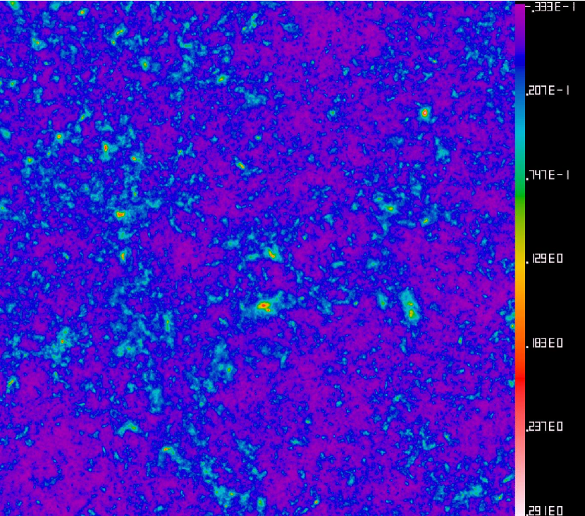
Figure 1: An initial noise-free $\kappa$ map in the N-body simulation of a $\Omega_{m}=$0.3 $\Lambda$CDM cosmology with a map width of 3.02 degrees and $2048^{2}$ pixels, and the scale is in units of $\kappa$.

We then simulate the CFHT Legacy Survey by adding noise to these clean maps. The noise $\kappa$ maps have a pixel-pixel variance $\sigma_{N}^{2}=\langle e^{2}\rangle/2/\langle N_{\rm pixel}\rangle$. Here $\langle e^{2}\rangle=0.47^{2}$ is the total noise estimated in the VIRMOS-DESCART survey and here we take it as what would be expected by the CFHT Legacy Survey. It includes the dispersion of the galaxy intrinsic ellipticity, PSF correction noise and photon shot noise. $\langle N_{\rm pixel}\rangle$ is the mean number of galaxies in each pixel. For VIRMOS, the number density of observed galaxies $n_{g}\simeq 26/{\rm arcmin}^{2}$, then $\langle N_{\rm pixel}\rangle=n_{g}[(\theta_{\kappa}/1^{{}^{\prime}})/N]^{2}$, where $N=2048$ is the number of grids by which we store 2D maps and the field of view $\theta_{\kappa}$ is in units of arc min. The factor of 2 arises from the fact that the shear field has two degrees of freedom ($\gamma_{1},\gamma_{2}$), where the definition of $\langle e^{2}\rangle$ sums over both. We use this as our best guess for the CFHT Legacy Survey noise. The maps we obtained through the method described above are non-periodic after the projection. In order to eliminate edge effects, we crop each smoothed map by a factor of $10\%$ in the margins of each $\kappa$ map for model with $\Omega_{m}=0.2$. For comparison, the size of maps for other models is the same as that of $\Omega_{m}=0.2$.

3 The optimal filter

Our goal is to find the optimal filter for constraining $\Omega_{m}$ by the non-Gaussianity of weak lensing. The non-Gaussianity of weak lensing for a clean map is quantified by the skewness $S_{3}$

$$S_{3}(\theta_{f})=\frac{\langle\kappa^{3}\rangle}{\langle\kappa^{2}\rangle^{2}},$$ (4)

where $\theta_{f}$ is the characteristic radius of the filter function. When noise is present, the definition of skewness can be modified to be (White & Hu (2000))

$$S_{3}(\theta_{f})=\frac{\langle\kappa_{\rm S+N}^{3}\rangle}{[\langle\kappa_{\rm S+N}^{2}\rangle^{2}-\kappa_{N}^{2}]^{2}}.$$ (5)

The subscript $S$ indicates a weak lensing signal while $N$ denotes random noise. Since $\langle\kappa_{\rm S+N}^{3}\rangle=\langle\kappa_{\rm S}^{3}\rangle$, $\langle\kappa_{\rm S+N}^{2}\rangle-\langle\kappa_{\rm N}^{2}\rangle=\langle\kappa_{\rm S}^{2}\rangle$, thus $S_{3}$ defined by Eq.5 is statistically equivalent to the one defined by Eq.4, and the presence of noise has only residual effects on the dispersion of $S_{3}$.

The skewness $S_{3}$ is a function of cosmological density parameters $\Omega_{m}$ and the filter function. The noise introduces a large dispersion in $S_{3}$ and also smears its intrinsic dependence on cosmological parameters. Filtering on a large scale reduces this noise, but also reduces the intrinsic skewness, and increases sample variance. Our goal is to find the optimal smoothing scale. Different filters also have different scale dependence,. The general form of this filter is hard to find, so we will employ five parametrized classes of filters in this paper. They are the top-hat (hereafter,TH), Gaussian (GS), aperture (AP), compensated Gaussian (CG) and Wiener (WN) filters, respectively. TH is normalized to have a sum unity in the 2D window function map, and GS is defined as $W(\theta)=(1/2\pi\theta_{f}^{2})\exp{(-\frac{\theta^{2}}{2\theta_{f}^{2}})}$ which is normalized by the same as TH. AP is defined as $W(\theta)=\frac{9}{\pi}(\frac{1}{\theta_{f}})^{2}[1-(\frac{\theta}{\theta_{f}})^{2}][1/3-(\frac{\theta}{\theta_{f}})^{2}]$ and zero for $\theta>\theta_{f}$, which has zero mean. The CG filter is written as $W(\theta)=\frac{1}{2\pi\theta_{f}^{2}}\left(1-\frac{\theta^{2}}{2\theta_{f}^{2}}\right)\exp\left(\frac{-\theta^{2}}{2\theta_{f}^{2}}+1\right)$, which holds zero area, and is normalized to have a peak amplitude of unity in Fourier space. This has the feature that it will only damp modes, and never amplify. Many analytic integrals for CG can be evaluated analytically (Crittenden et al., 2002). WN is defined in Fourier space by $W(l)=\frac{C_{s}(l)}{C_{s}(l)+C_{n}}$, where $C_{s}(l)$ is the angular power spectrum of the signal $\kappa$, while $C_{n}=\frac{4\pi\sigma_{N}^{2}f_{sky}}{N^{2}}$ is that for noise power, and $f_{sky}=\pi(\frac{\theta_{\kappa}}{360})^{2}$ is the fractional sky coverage of each map.

Given these filters, one can measure $S_{3}$ and its dispersion $\Delta S_{3}$, which are all functions of $\Omega_{m}$. $\Delta S_{3}$ causes the inferred $\Omega_{m}$ to differ from its true value by a change of $\Delta\Omega_{m}$. For each class of filter, there exists an optimal filter radius $\theta_{f}$ to minimize $\Delta\Omega_{m}$. Comparing the minimum $\Delta\Omega_{m}$ of each class of filter, one can then find the optimal one.

From simulated maps, we first calculate the skewness $S_{3}$ and its standard deviation $\Delta S_{3}$ with different filter radius for all kinds of cosmological models. The CFHT Legacy Survey will observe 160 square degrees, which is about 24 times larger than the simulated area. We conservatively decreased the error we obtained in the field-to-field variations by a factor of about 4 to estimate the sensitivity for the Legacy Survey. Therefore, the standard deviation of $S_{3}$ throughout this paper is taken to be one fourth of original predicted value from simulation. The skewness $S_{3}$ and its standard deviation $\Delta S_{3}$ of TH, GS, AP and CG window functions are shown in Fig.2 and 3, while that of WN filter are plotted in Fig.4. From Fig.2 and 4, it is shown that the expected $S_{3}$ decrease with the cosmological density parameter $\Omega_{m}$ for all of filters, which is in consistent with that predicted by perturbation theory at large $\theta_{f}$ (Gaztanaga & Bernardeau, 1998) and non-linear perturbation theory (Hui, 1999; Van Waerbeke et al., 2001). A fixed fluctuation amplitude measured by weak lensing is a smaller fractional fluctuation in a higher $\Omega_{m}$ universe, and thus less non-linear and less non-Gaussian. $S_{3}$ also decreases with filter scale $\theta_{f}$, as one would expect from the central limit theorem when smoothing over more independent patches to converge to a Gaussian distribution. Our dependence of $S_{3}$ agrees qualitatively with Van Waerbeke et al. (2001), where the detailed normalization depends on details of the redshift distribution. Estimates of $S_{3}$ are possible analytically. To optimize its measurement, we also need its standard deviation, which is related to a six point function. This is difficult to compute analytically.

The fit for $S_{3}$ in Fig.2 fails badly on not only small scale but large scales of more than 10 arc minutes. This is due to larger standard deviation of $S_{3}$ as shown in Fig.3 on both of the two scales. It is also apparent from Fig.3 that there exists an optimal filtering scale $\theta_{f}$ corresponding which minimizes $\Delta S_{3}$ (except for the WN filter that does not depend on filter radius). This is due to the trade-off between noise on small scales and sample variance on large scales. $S_{3}$ as a function of filter radius $\theta_{f}$ for the TH filter in Fig.2 is in rough agreement with that of White & Hu (2000) where cosmological model is specified to $\Omega_{m}=0.3$, but it differs from Jain et al. (2000). We do not understand the behaviour of the Gaussian window for large $\Omega$ at small angular scale, where a smoothing scale smaller than our resolution seems to be prefered. But we do not dwell on this since the Gaussian window is not observable on a shear map.

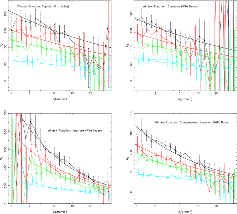
Figure 2: Skewness $S_{3}$ as a function of a smoothing scale $\theta_{f}$ for all window functions except for Wiener with cosmological models $\Omega_{m}=0.2$ (black line), $\Omega_{m}=0.3$ (red line), $\Omega_{m}=0.4$(green line) and $\Omega_{m}=1$ (blue line) respectively. The standard deviation of $S_{3}$ is taken to be one fourth of original predicted value from simulation, because the CFHT Legacy Survey will observe 160 square degrees, which is about 24 times larger than the simulated area. The smoother lines correspond to the best fit to $S_{3}$ for each model. For the purpose of discerning the error bars of different models, the plots of all models except for $\Omega_{m}=0.2$ are shifted in the direction of right. The simulated convergence $\kappa$ has added random noise.

Figure 3: $\Delta S_{3}$ as a function of a smoothing scale $\theta_{f}$ for all window functions except for Wiener with cosmological models $\Omega_{m}=0.2$ (solid line), $\Omega_{m}=0.3$ (dashed line), $\Omega_{m}=0.4$(dash-dotted line) and $\Omega_{m}=1$ (dotted line) respectively. The smoother lines correspond to the best fit to $\Delta S_{3}$ for each model.

Figure 4: Skewness $S_{3}$ (left panel) and standard deviation $\Delta S_{3}$ (right panel) as a function of cosmological parameter $\Omega_{m}$ for Wiener window function. The dashed lines indicate the best fit to $S_{3}$ and $\Delta S_{3}$ respectively. The error bars represent the same significance as Fig.2. The random noise is added to the simulated convergence $\kappa$.

From the above analyses, it is clear that $S_{3}$ and $\Delta S_{3}$ depend not only on the smoothing scale $\theta_{f}$ but also the cosmological parameter $\Omega_{m}$ for all window functions except for the WN filter. In real observations of weak lensing, one must evaluate the uncertainty in $\Omega_{m}$ for a given observed $S_{3}$ and $\Delta S_{3}$ to discriminate between cosmological models. One needs to invert the relation $S_{3}=S_{3}(\Omega_{m},\theta_{f})$ to obtain $\Omega_{m}=\Omega_{m}(S_{3},\theta_{f})$ and estimate the uncertainty of inferred $\Omega_{m}$ by

$$\Delta\Omega_{m}(S_{3}(\Omega_{m},\theta_{f}),\theta_{f})=\Omega_{m}(S_{3}(\Omega_{m},\theta_{f}),\theta_{f})-\Omega_{m}(S_{3}(\Omega_{m},\theta_{f})+\Delta S_{3}(\Omega_{m},\theta_{f}),\theta_{f}).$$ (6)

Because of the irregularity of the data points, the inversion is noisy and may introduce unrealistic artifacts. To overcome this problem, we first fit $S_{3}$ and $\Delta S_{3}$ by a combination of power laws of $\Omega_{m}$ and $\theta_{f}$ in the presence of noise, respectively

$$S_{3}(\Omega_{m},\theta_{f})=A(\Omega_{m})\theta_{f}^{B(\Omega_{m})},$$ (7)

and

$$\Delta S_{3}(\Omega_{m},\theta_{f})=A_{S}(\Omega_{m})\theta_{f}^{B_{S}(\Omega_{m})}+A_{N}(\Omega_{m})\theta_{f}^{B_{N}(\Omega_{m})},$$ (8)

where $A(\Omega_{m})=A_{1}\Omega_{m}^{B_{1}}$, $B(\Omega_{m})=A_{2}\Omega_{m}^{B_{2}}$, $A_{S}(\Omega_{m})=A_{S1}\Omega_{m}^{B_{S1}}$, $B_{S}(\Omega_{m})=A_{S2}\Omega_{m}^{B_{S2}}$, $A_{N}(\Omega_{m})=A_{N1}\Omega_{m}^{B_{N1}}$ and $B_{N}(\Omega_{m})=A_{N2}\Omega_{m}^{B_{N2}}$ respectively. The two terms of $\Delta S_{3}(\Omega_{m},\theta_{f})$ represent two sources of the dispersion of $S_{3}$: the intrinsic dispersion of signal and that caused by noise. Noise dominates at small smoothing scale, so we expect that $B_{N}(\Omega_{m})<0$, while we expect $B_{S}(\Omega_{m})>0$ because of the large smoothing behavior of $\Delta S_{3}$ from signal(Fig.3). For the Wiener function, we can just parameterize the dependence of skewness $S_{3}$ and its standard deviation $\Delta S_{3}$ on $\Omega_{m}$ as $S_{3}(\Omega_{m})=A_{1}\Omega_{m}^{B_{1}}$ and $\Delta S_{3}(\Omega_{m})=A_{2}\Omega_{m}^{B_{2}}$ respectively, because it is due to its independence of smoothing radius.

Table 1: Best Fit to $S_{3}$ and $\Delta S_{3}$ by Eq.(7) and Eq.(8)

	Top-hat	Gaussian	Aperture	Compensated Gaussian
$A_{1}$	62.16$\pm$1.21	65.79$\pm$1.11	252.74$\pm$4.01	90.33$\pm$0.69
$B_{1}$	-0.75$\pm$0.02	-0.64$\pm$0.01	-0.94$\pm$0.02	-0.81$\pm$0.01
$A_{2}$	-0.16$\pm$0.03	-0.17$\pm$0.02	-0.24$\pm$0.01	-0.18$\pm$0.01
$B_{2}$	-0.13$\pm$0.11	-0.07$\pm$0.09	-0.42$\pm$0.02	-0.43$\pm$0.03
$A_{S1}$	3.47$\pm$0.04	5.43$\pm$0.08	2.20$\pm$0.17	1.47$\pm$0.07
$B_{S1}$	-0.25$\pm$0.02	-0.07$\pm$0.03	-0.79$\pm$0.10	-0.71$\pm$0.05
$A_{S2}$	0.79$\pm$0.01	0.84$\pm$0.01	0.73$\pm$0.03	0.98$\pm$0.02
$B_{S2}$	0.10$\pm$0.02	-0.002$\pm$0.02	-0.06$\pm$0.04	0.23$\pm$0.03
$A_{N1}$	12.18$\pm$1.75	7.02$\pm$0.86	380.75$\pm$108.86	8.11$\pm$1.60
$B_{N1}$	-0.79$\pm$0.13	-0.62$\pm$0.12	-1.05$\pm$0.23	-0.98$\pm$0.17
$A_{N2}$	-0.42$\pm$0.09	-0.05$\pm$0.05	-1.90$\pm$0.15	-0.87$\pm$0.17
$B_{N2}$	-0.43$\pm$0.18	-1.78$\pm$0.45	-0.14$\pm$0.07	-0.35$\pm$0.14

We fit the relation of $S_{3}$ and $\Delta S_{3}$ with a function of $\Omega_{m},\theta_{f}$ by Eqs.(7) and (8) for all filters except for WN. Their best fit coefficients $A_{S1},B_{S1},A_{S2},B_{S2},A_{N1},B_{N1}$, $A_{N2},B_{N2}$ are listed in Table LABEL:table:fit respectively, the best fit relations of which are also plotted with smoother lines in Fig.2 and 3. For the WN filter, the best fit coefficients $A_{1}=68.03\pm 2.37$, $B_{1}=-0.67\pm 0.03$, $A_{2}=18.17\pm 6.13$ and $B_{2}=-0.35\pm 0.26$, and the dashed lines in Fig.4 show the best fit to $S_{3}$ and $\Delta S_{3}$. In the fit of skewness $S_{3}$, we weighted using the standard deviation of the skewness. Using these best fit coefficients, we can calculate the $\Delta\Omega_{m}$ with the function of $\Omega_{m}$ and $\theta_{f}$, which are shown in Fig.5 and 6. As expected, we find in Fig.5 that there does exist an optimal smoothing scale for each class of filter (except for the WN filter) that has a minimum error for the inferred $\Omega_{m}$. This optimal smoothing scale has only a weak dependence on cosmology except for GS filter. The minimum $\Delta\Omega_{m}$ decreases toward lower $\Omega_{m}$. Due to the $S_{3}\propto\Omega_{m}^{\sim-0.8}$ behavior (Table LABEL:table:fit), at low $\Omega_{m}$, a small change of $\Omega_{m}$ results in a large change of $S_{3}$. But $\Delta S_{3}$ does not have such strong $\Omega_{m}$ dependence, thus the resulting error in $\Omega_{m}$ decreases toward lower $\Omega_{m}$. In addition, we show in Fig.6 the relative uncertainty $\Delta\Omega_{m}/\Omega_{m}$ as a function of $\Omega_{m}$ smoothed at the optimal filter radius for all of filters respectively. It is shown that the relative uncertainty $\Delta\Omega_{m}/\Omega_{m}$ for the Compensated Gaussian filter almost stays constant with $\Omega_{m}=0.1$, and takes the smallest value in the range from $\Omega_{m}=0.2$ to 0.6 of interest compared with that of other filters. By comparing the minimum of $\Delta\Omega_{m}$ for each filter class, we then conclude that the compensated Gaussian filter to be the optimal filter for all cosmologies. The relative uncertainty $\Delta\Omega_{m}/\Omega_{m}$ at the optimal filter scale for this filter is nearly independent of $\Omega_{m}$, and the corresponding optimal filter scale is about 2.5 arc minutes.

Figure 5: $\Delta\Omega_{m}$ as a function of a smoothing scale $\theta_{f}$ for all except for Wiener window function with cosmological models $\Omega_{m}=0.2$ (solid line), $\Omega_{m}=0.3$ (dashed line), $\Omega_{m}=0.4$(dash-dotted line) and $\Omega_{m}=1$ (dotted line) respectively. The simulated convergence $\kappa$ is added with random noise.

Figure 6: The relative uncertainty $\Delta\Omega_{m}/\Omega_{m}$ as a function of $\Omega_{m}$ smoothed at the optimal filter radius for Top-hat(solid line), Gaussian(dashed line), Aperture(dash-dotted line), Compensated Gaussian(dotted line) and Wiener(dash-tridotted line) filters respectively.

4 Conclusions

We have studied the power of weak lensing surveys to measure the matter density of the universe without relying on any exterior data sets. We found that the CFHT Legacy Survey can measure a fractional accuracy in $\Omega_{m}$ of 10%, which is competitive with global joint analyses, but bypasses a large number of cross calibration uncertainties.

We ran a series of high resolution N-body simulation to study statistical skewness properties of weak lensing by large-scale structure in the universe with a range of cosmological matter density parameters. We added noise due to intrinsic ellipticity of background faint galaxies to the simulated $\kappa$ fields and smoothed it using different filters with a range of smoothing radii. We calculated the skewness $S_{3}$ of the smoothed $\kappa$ field with added Gaussian noise and predicted the uncertainty $\Delta\Omega_{m}$ for the cosmological mass density parameter for a given $S_{3}$ and smoothing radius $\theta_{f}$. We examined the relative discriminating power of different window functions for distinguishing cosmological models in the upcoming CFHT Legacy Survey. Except for the Wiener filter, we found the optimal smoothing radius for all of four window functions that minimizes $\Delta\Omega_{m}$. This optimal smoothing scale has only a weak dependence on cosmology. The compensated Gaussian function was the optimal filter for measuring $\Omega_{m}$ from skewness. The relative uncertainty $\Delta\Omega_{m}/\Omega_{m}$ smoothed at the optimal filter radius for Compensated Gaussian filter is about 10%.

To overcome the irregularity of the simulated $S_{3}$ and $\Delta S_{3}$, we have fitted their smoothing scale and cosmology dependence with some phenomenological power laws. One could derive these relations analytically using perturbation theory following the theoretical work of Bernardeau et al. (1997). But since skewness is intrinsically non-linear, such a perturbation approach has to be tested against simulations. In fact, in our work based on simulations, the optimal filter radius is a few arc minutes or $\sim 1$ Mpc/h, which lies in strongly non-linear regime, where perturbation theory breaks down (Gaztanaga & Bernardeau, 1998). In the non-linear regime, a semi analytical model, hyperextended perturbation theory (hereafter HEPT) (Scoccimarro & Frieman, 1999), which applies at the highly non-linear regime, and a fitting formula to interpolate between the quasi-linear and highly non-linear regime (Scoccimarro & Couchman, 2001), have been applied to predict $S_{3}$ (Hui, 1999; Van Waerbeke et al., 2001). Since these models reply on simulations for calibration, they by no means can produce better result than simulations. Furthermore, to calculate the lensing $\Delta S_{3}$ analytically, one has to know the $S_{6}$ of the density field, which can be predicted by HEPT but has not been tested against simulations (Scoccimarro & Frieman, 1999). So we’d rather using our fitting formula approach instead of adopting these analytical results.

We thank an anonymous referee for several helpful suggestions on the manuscript. T.J.Zhang would like to thank CITA for its hospitality during his visit. The research was supported in part by NSERC and computational resources of the CFI funded infrastructure. P.J.Zhang thanks the department of astronomy & astrophysics and CITA of University of Toronto where part of the work was done. P.J.Zhang is supported by the DOE and the NASA grant NAG 5-10842 at Fermilab.

References

- Bacon et al. (2000) Bacon, D. J., Refregier, A. R., & Ellis, R. S. 2000, MNRAS, 318, 625
- Bernardeau et al. (2002) Bernardeau, F., Mellier, Y., & van Waerbeke, L. 2002, A&A, 389, L28
- Bernardeau et al. (1997) Bernardeau, F., van Waerbeke, L., & Mellier, Y. 1997, A&A, 322, 1
- Blanchard et al. (2003) Blanchard, A., Douspis, M., Rowan-Robinson, M., & Sarkar, S. 2003, ArXiv Astrophysics e-prints, 4237
- Blandford et al. (1991) Blandford, R. D., Saust, A. B., Brainerd, T. G., & Villumsen, J. V. 1991, MNRAS, 251, 600
- Brown et al. (2002) Brown, M. L., Taylor, A. N., Bacon, D. J., Gray, M. E., Dye, S., Meisenheimer, K., & Wolf, C. 2002, in eprint arXiv:astro-ph/0210213, 10213–+
- Contaldi et al. (2003) Contaldi, C. R., Hoekstra, H., & Lewis, A. 2003, ArXiv Astrophysics e-prints, 2435
- Crittenden et al. (2002) Crittenden, R. G., Natarajan, P., Pen, U., & Theuns, T. 2002, ApJ, 568, 20
- Gaztanaga & Bernardeau (1998) Gaztanaga, E. & Bernardeau, F. 1998, A&A, 331, 829
- Gunn (1967) Gunn, J. E. 1967, ApJ, 147, 61
- Hamana et al. (2002) Hamana, T., Miyazaki, S., Shimasaku, K., Furusawa, H., Doi, M., Hamabe, M., Imi, K., Kimura, M., Komiyama, Y., Nakata, F., Okada, N., Okamura, S., Ouchi, M., Sekiguchi, M., Yagi, M., & Yasuda, N. 2002, in eprint arXiv:astro-ph/0210450, 10450–+
- Hoekstra et al. (2002) Hoekstra, H., Yee, H. K. C., Gladders, M. D., Barrientos, L. F., Hall, P. B., & Infante, L. 2002, ApJ, 572, 55
- Hui (1999) Hui, L. 1999, ApJ, 519, L9
- Jain et al. (2000) Jain, B., Seljak, U., & White, S. 2000, ApJ, 530, 547
- Jarvis et al. (2002) Jarvis, M., Bernstein, G., Jain, B., Fischer, P., Smith, D., Tyson, J. A., & Wittman, D. 2002, in eprint arXiv:astro-ph/0210604, 10604–+
- Juszkiewicz et al. (1995) Juszkiewicz, R., Weinberg, D. H., Amsterfamski, P., Chodorowski, M., & Bouchet, F. 1995, ApJ, 442, 39
- Kaiser (1992) Kaiser, N. 1992, ApJ, 388, 272
- Miralda-Escude (1991) Miralda-Escude, J. 1991, ApJ, 380, 1
- Nusser & Dekel (1993) Nusser, A. & Dekel, A. 1993, ApJ, 405, 437
- Pen et al. (1994) Pen, U., Spergel, D. N., & Turok, N. 1994, Phys. Rev. D, 49, 692
- Pen et al. (2003) Pen, U., Zhang, T., Waerbeke, L. v., Mellier, Y., Zhang, P., & Dubinski, J. 2003, in eprint arXiv:astro-ph/0302031, 2031–+
- Refregier et al. (2002) Refregier, A., Rhodes, J., & Groth, E. J. 2002, ApJ, 572, L131
- Scoccimarro & Couchman (2001) Scoccimarro, R. & Couchman, H. M. P. 2001, MNRAS, 325, 1312
- Scoccimarro & Frieman (1999) Scoccimarro, R. & Frieman, J. A. 1999, ApJ, 520, 35
- Seljak & Zaldarriaga (1996) Seljak, U. & Zaldarriaga, M. 1996, ApJ, 469, 437+
- Spergel et al. (2003) Spergel, D. N., Verde, L., Peiris, H. V., Komatsu, E., Nolta, M. R., Bennett, C. L., Halpern, M., Hinshaw, G., Jarosik, N., Kogut, A., Limon, M., Meyer, S. S., Page, L., Tucker, G. S., Weiland, J. L., Wollack, E., & Wright, E. L. 2003, ArXiv Astrophysics e-prints, 2209
- Tegmark & Zaldarriaga (2002) Tegmark, M. & Zaldarriaga, M. 2002, Phys. Rev. D, 66, 103508
- Van Waerbeke et al. (2001) Van Waerbeke, L., Hamana, T., Scoccimarro, R., Colombi, S., & Bernardeau, F. 2001, MNRAS, 322, 918
- Van Waerbeke et al. (2002) Van Waerbeke, L., Mellier, Y., Pelló, R., Pen, U.-L., McCracken, H. J., & Jain, B. 2002, A&A, 393, 369
- White & Hu (2000) White, M. & Hu, W. 2000, ApJ, 537, 1