Does the small CMB quadrupole moment suggest new physics?

Abstract:

Motivated by WMAP’s confirmation of an anomalously low value of the quadrupole moment of the CMB temperature fluctuations, we investigate the effects on the CMB of cutting off the primordial power spectrum $P(k)$ at low wave numbers. This could arise, for example, from a break in the inflaton potential, a prior period of matter or radiation domination, or an oscillating scalar field which couples to the inflaton. We reanalyze the full WMAP parameter space supplemented by a low-$k$ cutoff for $P(k)$. The temperature correlations by themselves are better fit by a cutoff spectrum, but including the $TE$ temperature-polarization spectrum reduces this preference to a 1.4$\sigma$ effect. Inclusion of large scale structure data does not change the conclusion. If taken seriously, the low-$k$ cutoff is correlated with optical depth so that reionization occurs even earlier than indicated by the WMAP analysis.

1 Introduction

One of the intriguing results of the Wilkinson Microwave Anisotropy Probe (WMAP) is a smaller than expected correlation of temperature fluctuations on large angular scales, corresponding to a low value for the quadrupole moment. Figure 1 shows the WMAP results for $C(\theta)$ and the low-multipole $C_{l}$’s. Their “Basic results” paper [1] states that the “probability of so little $C(\theta>60^{\circ})$ anisotropy power is $\sim 2\times 10^{-3}$, given the best-fit [running spectral index] $\Lambda$CDM model.” (See also refs. [2, 3] for related discussions.) Given the large uncertainties in this region due to cosmic variance, one might never know whether this constitutes a truly significant deviation from standard cosmological expectations. However it has recently been suggested that measuring polarization from galaxy clusters may in the next decade give a complementary determination of the quadrupole moment [4] and its evolution with redshift.

Figure 1: Left: Angular correlation function $C(\theta)$ for CMB temperature anisotropy, from fig. 13 of [1]. Our plot of WMAP TT multipole data (from http://lambda.gsfc.nasa.gov/product/map/ map$\_$tt$\_$powspec.cfm) with the best fit $\Lambda$CDM model (with constant scalar index $n_{s}$) from table 7 of [15]. Cosmic variance is a factor of $1\pm 1/\sqrt{l+1/2}$.

Loss of power at large angles could be explained by lowering the primordial power spectrum of inflaton fluctuations $(P(k))$ at small wave numbers. Prior to the WMAP observation, there have been several suggestions for generating such an effect. Sharp features in the inflaton potential [5]-[7] can suppress power at low $k$. Recently [8] studied two other possibilities: an oscillating scalar field $\chi$ coupling to the inflaton can temporariliy suppress inflaton fluctuations, leading to a cutoff at low $k$; a prior period of matter or radiation domination before the beginning of inflation has a similar effect [9]. Spatial compactness [10] or curvature [11] can also lead to a smaller CMB quadrupole moment. These scenarios require that the total amount of inflation is close to the minimum amount required to solve the horizon and flatness problems, or alternatively that the break in the inflaton potential is reached just when the relevant scales are crossing the horizon.

Recent papers [12, 13] considered how cutting off $P(k)$ at low $k$ can improve the fit to the data. Ref. [13] found that the data favor having such a modified primordial spectrum at the $2\sigma$ level, whereas [12] obtain weaker evidence for a cutoff. The conclusion of ref. [13] was based upon using only the temperature anisotropy data, and ignoring polarization. The TE cross power spectrum represents one third of the total data set, and has an important effect on the determination of parameters that would lower the TT quadrupole moment. If one simply cuts off $P(k)$ at low $k$ while keeping all other cosmological parameters fixed, the improvement of the fit to the TT spectrum is accompanied by a deterioration in the fit to the TE spectrum, such that the overall improvement of the fit is nil. To counteract this, one needs to allow other parameters like the optical depth $\tau$ and the fraction of dark energy $\Omega_{\Lambda}$ to vary. In the present study, we do a complete likelihood analysis in which all the relevant cosmological parameters are varied in order to find those values which have the real maximum likelihood. We corroborate and extend the results of [12], who used a similar approach.

In the second section we describe the theoretical models which can lead to a suppression of low-$k$ power in the primordial fluctuations. Section three presents our likelihood analysis, in which we find that the preference for a cutoff in $P(k)$ is of marginal statistical significance. Our findings and conclusions are summarized in the final section.

2 Theoretical Models

There are many ways to alter the spectrum of inflaton fluctuations relative to the flat Harrison-Zeldovich form. Here we will concentrate only on those that produce a sharp reduction in large wavelength power, needed to suppress the low multipoles of the CMB. One way is to engineer the inflaton potential $V(\phi)$, which in principle can yield any desired form for $P(k)$ [5, 14]. A model which predicts a step-like feature in $P(k)$ was proposed by Starobinsky [6], which assumes that there is a sudden change in the slope of $V(\phi)$. If by chance the scales presently corresponding to large-angle CMB anisotropies exit the Hubble radius at the moment when $\phi$ crosses the kink in $V(\phi)$, then the power of smaller $k$ fluctuations which subsequently cross the horizon can be suppressed. The resulting power spectrum (shown in [7]) looks similar to the one we shall discuss below in fig. 2b.

More recently (but before WMAP’s data release) ref. [8] investigated possible effects of a limited duration of inflation on the power spectrum of the inflaton fluctuations. Two of these predicted that $P(k)$ should be strongly suppressed at low wave numbers. The first was in the context of the hybrid inflation model, with Lagrangian

$$-{\cal L} = \sqrt{-g}\Bigl{[}{\textstyle{1\over 2}}\partial_{\mu}\phi\,\partial^{\mu}\phi+{\textstyle{1\over 2}}\partial_{\mu}\chi\,\partial^{\mu}\chi+V(\phi,\chi)\Bigr{]},$$ (1)

$$\hbox{with}\qquad V(\phi,\chi) = {\textstyle{1\over 2}}\,m^{2}\,\phi^{2}+{\textstyle{1\over 4}}\,\lambda(\chi^{2}-v^{2})^{2}+{\textstyle{1\over 2}}\,g\,\chi^{2}\phi^{2}+{\textstyle{1\over 12}}\,\tilde{\lambda}\,\phi^{4}.$$

It was noticed that if the field $\chi$, which is responsible for triggering the end of inflation, is oscillating prior to horizon crossing of the relevant inflaton fluctuations, these oscillations can strongly affect $P(k)$ for $k$ values which are below some characteristic scale $k_{\rm max}$, defined by

$$k_{\rm max}=Me^{-Ht_{0}}$$ (2)

Here $M$ is the $\chi$ field mass, and $t_{0}$ is the amount of time prior to horizon crossing of the mode $k$ during which $\chi$ was oscillating. In fact there are two important scales, this one, which comes about because the $\chi$ oscillations cause production of inflaton fluctuations, and a lower one, below which the fluctuations are suppressed. The suppression occurs because the average value of $g\chi^{2}$ contributes to the squared mass of the inflaton, $\delta m^{2}_{\phi}=\langle g\chi^{2}\rangle=\frac{1}{2}g\chi_{0}^{2}e^{-3Ht}$. When $\delta m^{2}_{\phi}\mbox{\raisebox{-2.58334pt}{~{}$\stackrel{{\scriptstyle>}}{{\sim}}$~{}}}H^{2}$, the inflaton rolls quickly, which suppresses fluctuations on scales $k$ which have not yet crossed the horizon. However, the amplitude of $\chi$ redshifts exponentially, and at a certain time $\delta m^{2}_{\phi}$ will fall below $H^{2}$. Fluctuations which have not yet frozen out by this time will have a chance to grow toward their normal amplitude, $\delta\phi(k)=H/2\pi$; thus larger wave numbers will be unchanged by this effect. The fractional amount by which $P(k)$ is reduced at low $k$ is $g\chi_{0}^{2}/H^{2}$ for small values of this parameter, where $\chi_{0}$ is the initial amplitude of the $\chi$ oscillations, and $H$ is the Hubble parameter during inflation. For large values of $g\chi_{0}^{2}/H^{2}$, the suppression is essentially complete, $P(k)\cong 0$. This is illustrated for some typical parameter values in figure 2a.

The second situation studied in [8] is that in which the inflaton fluctuations with wave number $k$ cross the horizon shortly after the beginning of inflation, where the inflationary epoch is preceded by matter or radiation domination [9]. In this case, power is suppressed on scales below $k\sim H$, the only relevant scale in the problem. (This refers to the value of $k$ at the time when inflation starts. The physical wave number gets reduced by the subsequent inflation.) The deformation of the power spectrum has a unique form, which is shown in figure 2b for the case of prior matter domination. The suppression of $P(k)$ in this case is a factor of $0.063$.

Figure 2: (a) Effect of $\chi$ oscillations on $P(k)$ for $M=50H$, $g\chi_{0}^{2}/e^{3Ht_{0}}=0.003H^{2}$, $t_{0}=4/H$. $P(k)$ is normalized such that $P(k)=1$ for a flat Harrison-Zeldovich spectrum. (b) Effect of prior period of matter domination on $P(k)$. The normalization of $k$ is in fact arbitrary—see discussion at beginning of section 3.

Both of the above effects rely upon having a limited period of inflation: inflation must not have started much earlier than the time when the large-angle CMB fluctuations first crossed the inflationary horizon. For the oscillating scalar scenario, this is because its oscillations are quickly Hubble damped. After at most 30 e-foldings of inflation, the amplitude of $\chi$ will be too small to have any further effect on the CMB. In the second scenario, there must be a coincidence of scales such that the large angle fluctuations cross the horizon just at the beginning of inflation; in this case inflation can last no longer than the minimum duration needed for solving the horizon and flatness problems.

3 Effect on CMB temperature fluctuations

Let us consider the effect of the spectrum shown in fig. 2b on the CMB temperature anisotropy. The physical scale of wave numbers at which $P(k)$ changes is determined by the total amount of inflation following the horizon crossing of the corresponding mode, denoted by $k=H$ in fig. 2b. A longer period of inflation stretches the wavelength of this mode to larger physical values. We refer to this model-dependent cutoff scale as $k_{*}$. Figure 3 shows the effect of varying $k_{*}$ in a modified version of the CMBFAST code [16] which incorporates the distorted spectrum. There it is seen that the relevant scales for suppressing the lowest multipoles are on the order of $k_{*}\sim$ a few $\times 10^{-4}$ Mpc^-1. As noted in [12, 13], even a sharp cutoff in $P(k)$ does not generate a sharp rise in the temperature multipoles since the latter are a convolution of the former of the form $C_{l}\sim\int dkk^{-1}j_{l}^{2}(k[\eta_{0}-\eta_{\rm dec}])P(k)$.

Figure 3: Effect of prior period of matter domination on temperature anisotropy. The cutoff wave number $k_{*}$ is in units of Mpc^-1.

If we ignore the TE polarization data, it is possible to obtain a better fit to the measured WMAP anisotropy in the manner shown in fig. 3. However, if one changes $P(k)$ like this without altering any other parameters, it exacerbates the fit to the TE spectrum. Figure 4a shows the experimental data at low $l$ [17]; fig. 4b shows that larger values of the cutoff wave number $k_{*}$ suppress the low TE multipoles in conflict with experimental observation of stronger power at low $l$. The strong TE signal at low $l$ is the basis for WMAP’s inference of a large optical depth $\tau$ and early reionization, which shows that $\tau$ is an important parameter to vary in order to try to repair the damage to the fit to TE done by modifying $P(k)$. However changing $\tau$ can also hurt the agreement between data and theory for the higher multipoles unless the scalar spectral index $n_{s}$ is also adjusted to compensate the change in $\tau$.

Figure 4: (a) WMAP TE cross polarization spectrum (fig. 8 of [17]). (b) Suppression of TE spectrum by $P(k)$ with low-$k$ cutoff $k_{*}$.

This kind of reasoning suggests that no safe conclusions can be drawn without doing a complete analysis in which at least a minimal set of cosmological parameters (like the six-dimensional parameter space considered in [1, 15]) are allowed to vary. We have therefore generated grids of theoretical power spectra with varying values for $\omega_{b}\equiv\Omega_{b}h^{2}$, $\omega_{m}\equiv\Omega_{m}h^{2}$, $h$, $\tau$, $A_{s}$, $n_{s}$ and for the cutoff scale $k_{*}$, using several forms for the cutoff spectrum $P(k)$. We fixed to zero some parameters which are not strictly necessary for fitting the WMAP data, like the spatial curvature or the amount of primordial gravitational waves. In the following, the minimum $\chi^{2}$ values have been found using a Powell minimization algorithm. For models which do not match one of the grid points, our code first computes the power spectra $C_{l}^{TT}$, $C_{l}^{TE}$, $P(k)$ by cubic interpolation between the grid’s neighboring points, and then calculates the corresponding $\chi^{2}$ value. We checked that for our grid spacing, the interpolation is always accurate to one per cent. To be sure that we understand the results of ref. [13], we started with their ansatz

$$P(k)=A_{s}(1-e^{-(k/k_{*})^{\alpha}})k^{n_{s}-1}$$ (3)

where $\alpha=3.35$ is chosen to match the shape at low $k$ of a model similar to that shown in fig. 2b (they considered a period of prior kination rather than matter domination). We performed comparisons with three different data sets: WMAP TT power spectrum alone, WMAP TT and TE combined spectra, and WMAP TT$+$TE supplemented by large scale structure data from the 2 degree field (2dF) galaxy redshift survey [18]. For WMAP, we computed the likelihood of a given model using the software provided by the collaboration and described in [19]. For the 2dF power spectrum, we used the window functions and correlation matrix available at http://msowww.anu.edu.au/2dFGRS/.

First, we verify that there is some preference for a nonvanishing cutoff in $k$ space when only the temperature data is included. Figure 5 shows the likelihood (normalized to 1 at the best fit value) for $k_{*}$, having marginalized over the other parameters. The model without a cutoff is excluded only at the 90% confidence level ($\Delta\chi^{2}\simeq 2.6$), which is not very significant. We note that artificially changing the first three theoretical multipoles, so as to exactly match the first three data points, improves $\chi^{2}$ by 7.0, corresponding to a Bayesian confidence level of more than 99%. Had we been able to achieve such a large $\Delta\chi^{2}$, we would have been more convinced that there is some evidence for a cutoff power spectrum in the temperature data.

We obtain a smaller preferred value of $k_{*}\cong 0.0003$ Mpc^-1 than did ref. [13], who found $k_{*}\cong 0.0005$ Mpc^-1. We have verified explicitly that this discrepancy is due to their having done the analysis on a smaller grid, in a restricted subspace of the parameters, which does not include the true minimum $\chi^{2}$. Ref. [13] only explored the space of the parameters which have a direct effect on the low–multipole temperature spectrum, namely the primordial parameters $A_{s}$, $n_{s}$, $k_{*}$ and the cosmological constant $\Omega_{\Lambda}$ (which can be re-expressed in our basis as $\Omega_{\Lambda}=1-\omega_{m}/h^{2}$). Other parameters were kept fixed at $\omega_{m}=0.135$, $\omega_{b}=0.022$, $\tau=0.17$. These constraints correspond to the best-fit values (with a running $n_{s}$) for the “WMAPext+2dFGRS” data set which includes data from other CMB experiments and large scale structure measurements. A priori, there is no justification for imposing such constraints on a smaller data set (WMAP TT alone). For instance, we find that in the absence of a cutoff ($k_{*}=0$), the maximum likelihood in the full six-dimensional parameter space has an effective $\chi^{2}$ of 972 for 893 degrees of freedom, while imposing the previous constraints raises the best $\chi^{2}$ to 979. When polarization and large scale structure data are included in the analysis, fig. 5 shows that the evidence for a cutoff spectrum gets even weaker, while values of $k_{*}$ bigger than $5\times 10^{-4}$ Mpc^-1 are now excluded at $2\sigma$.

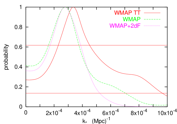
Figure 5: Likelihood of the wave number cutoff $k_{*}$ for WMAP TT, TT$+$TE and TT$+$TE$+$2dF data sets. The TT curve has a slightly higher preferred $k_{*}$ relative to the other two. The horizontal lines refer to the 1$\sigma$ (68 %) and 2$\sigma$ (95 %) confidence levels.

To see how parameters are correlated, in fig. 6 we also show confidence regions in the $\tau$-$k_{*}$ plane for the three different data sets, and the maximum likelihood value of each parameter for fixed values $k_{*}$. Using TT alone (fig. 6a), the preference for nonzero $k_{*}$ is only slightly bigger than a $1\sigma$ effect. When TE polarization data is included (fig. 6b), the significance is further reduced, and the anticipated need for larger optical depth values is manifested. By examining the most likely values of the other parameters as a function of $k_{*}$, fig. 6d, we see that an increase in $k_{*}$ and $\tau$ can be compensated by an increase in $n_{s}$, $h$, $\omega_{b}$, and a decrease in $\omega_{\rm cdm}$. Inclusion of large scale structure data (fig. 6c) breaks this degeneracy, but does not much improve the low statistical significance of the determination of $k_{*}$.

Figure 6: (a)-(c): 1 and 2 $\sigma$ confidence regions in the $\tau$-$k_{*}$ plane for WMAP TT, TT$+$TE and TT$+$TE$+$2dF data sets. (d) Most probable values of other parameters as a function of $k_{*}$, in the case of the TT$+$TE$+$2dF data sets.

To give a more precise idea of the statistical significance, we tabulate the best fit parameters and $\chi^{2}$ of the fit for the three cases in Table 1. As expected, the TT data by themselves show the strongest preference for a cutoff, but the change in $\chi^{2}$ is still only 2.6. When the TE data are included $\Delta\chi^{2}$ falls to 1.8. With the inclusion of 2dF data, $\Delta\chi^{2}=2.0$. Thus the model with no cutoff is within $1.4\sigma$ of the minimum $\chi^{2}$ point.

parameter	WMAP best fit	WMAP TT		TT$+$TE		TT$+$TE$+$2dF
	$\Lambda$CDM model	$k_{*}=0$	$k_{*}\neq 0$	$k_{*}=0$	$k_{*}\neq 0$	$k_{*}=0$	$k_{*}\neq 0$
$k_{*}/10^{-4}$Mpc-1	$-$	$-$	3.4	$-$	2.7	$-$	2.8
$\Omega_{b}h^{2}$	0.023	0.023	0.023	0.023	0.023	0.023	0.023
$\Omega_{m}h^{2}$	0.15	0.15	0.15	0.15	0.15	0.14	0.14
$h$	0.68	0.69	0.69	0.69	0.70	0.71	0.71
$\tau$	0.11	0	0	0.11	0.12	0.13	0.14
$n_{s}$	0.97	0.95	0.95	0.97	0.97	0.97	0.98
${\chi^{2}}^{\phantom{1}}$	1431	972.2	969.6	1431.3	1429.5	1458.7	1456.7
d.o.f.	1342	893	892	1342	1341	1374	1373

Table 1: Maximum likelihood parameters for the three different data sets, with and without cutoff $k_{*}$. WMAP best fit is from table 1 of [15].

The above results were obtained using the ansatz (3) for $P(k)$. We repeated the analysis for primordial spectra of the forms shown in figs. 2a and 2b, as well as a sharp step-function cutoff. They give no better nor worse a fit relative to (3).

4 Summary and conclusions

We have investigated whether the anomalously small power of large-angle CMB temperature anisotropies is indicative of new physics that could suppress the primoridal power spectrum of inflaton fluctuations at low wave number by introducing a cutoff $k_{*}$. We analyzed the complete WMAP data set including polarization, with and without the addition of the 2dF galaxy power spectrum data. Allowing for a variation of the six standard cosmological parameters characterizing a spatially flat universe, we find a marginal preference for a nonvanishing cutoff scale of $k_{*}=(2.7\pm 1)\times 10^{-4}$ Mpc^-1, in agreement with ref. [12]. Like them we find that the likelihood is nongaussian for low $k$ (fig. 5) so that $k_{*}$ is bounded to be above zero at a confidence level of only $59-64$ % (depending upon whether 2dF data is included). By contrast, ref. [13] finds $k_{*}>0$ at the $87-93$ % c.l. Moreover their most likely value of $k_{*}$ is larger than ours, $(4.9\pm 1)\times 10^{-4}$ Mpc^-1. We have explained the reasons for the differences between these results and our own.

Thus we conclude that at present the motivation from the low quadrupole and octopole moments for a power spectrum with an infrared cut-off is quite weak. Nevertheless we have pointed out correlations between the parameters which will be relevant for fitting the low quadrupole with such models. In particular there is a tendency for optical depth $\tau$ to increase in order that the low-$l$ polarization data remain consistent with the model in the presence of a low-$k$ cutoff.

How can we reconcile the small statistical significance of the need for a cutoff with the WMAP collaboration’s statement that the probability of having such low power at large angles is only $2\times 10^{-3}$? The answer lies in the highly nonGaussian nature of the likelihood function for the $C_{l}$’s [19, 20]. Expressing the temperature anisotropy as $\delta T=\sum_{lm}a_{lm}Y_{lm}(\phi,\theta)$, the $a_{lm}$’s have a Gaussian distribution, but the multipole moments, $C_{l}=\sum_{m}\langle|a_{lm}|^{2}\rangle$, have the distribution [21]

$${dP\over dC_{l}}\ \propto\ x^{l-1/2}e^{-(l+1/2)x}\,;\qquad x\equiv{C_{l}^{\rm obs}\over C_{l}^{\rm theo}}.$$ (4)

For large $l$ this can be well-approximated by a Gaussian, but for low $l$ it is quite asymmetric about the average value $x=1$. From this fact we can easily reconcile the small probability $2\times 10^{-3}$ with the lack of a significant improvement in the $\chi^{2}$ when considering models with cutoff power spectra, as we now explain.

Let us review the method which was used to arrive at WMAP’s small probability, as described in section 7 of [15]. From a large ensemble of models in the vicinity of the maximum likelihood model, one generates simulations of the data which include the effects of cosmic variance and the sky cut which is applied to the actual WMAP observations. Among these realizations, one then counts the number whose value of the quadrupole moment $C_{2}$ is less than or equal to the measured $C_{2}^{\rm obs}$, and compares to the total number in the ensemble. If we neglect the experimental noise (which is much smaller than cosmic variance at l=2) and the sky cut (which correlates the quadrupole with other multipoles), then for the quadrupole this amounts to computing

$$P[C_{2}<C_{2}^{\rm obs}]={\int_{0}^{0.1}dx{dP\over dC_{2}}\over\int_{0}^{\infty}dx{dP\over dC_{2}}}\cong 0.008$$ (5)

where we used the observed value $C_{2}^{\rm obs}=123$ and the theoretical one $C_{2}^{\rm theo}=1200$. Evidently inclusion of the “experimental complications” decreases this probability somewhat, but at least we can roughly understand its small order of magnitude.

Such an analysis could in principle be repeated including a cutoff power spectrum. We can roughly anticipate the results using the same approximation as in equation (4.2), but replacing the $\Lambda$CDM integration bound $x_{\Lambda{\rm CDM}}=0.1$ by $x_{k_{*}}\simeq 0.2$, since the cutoff model is able to reduce the theoretical quadrupole by about a factor of 2 (further reduction comes at the expense of dragging down the higher multipoles too much). Then we would obtain $P[C_{2}<C_{2}^{\rm obs}]=0.04$. This is a five-fold increase over the low probability in (5), but it is still low. Neither model satisfactorily explains the observed low quadrupole, unless large statistical fluctuations are invoked. Because of the nongaussianity of the likelihood function, only a much more radical suppression of $C_{l}^{\rm theo}$ could significantly increase this probability.

This explains why in our Bayesian analysis, we do not see a big difference between the best $\chi^{2}$ value for $k_{*}\neq 0$ and that for $k_{*}=0$. In this approach, we are making a different comparision, namely:

$$\Delta\chi^{2}\sim-2\left(\ln{dP\over dC_{2}}(x_{\Lambda\rm CDM})-\ln{dP\over dC_{2}}(x_{k_{*}})\right)\cong-1.6$$ (6)

This crude estimate does not replace the global seven-parameter analysis that we performed, but it gives a very good approximation for the improvement in $\chi^{2}$ which we find. From this argument we conclude that there is no real discrepancy between WMAP’s low probability $2\times 10^{-3}$ and the seemingly much higher probability found by us and by [3, 12, 13]. However we also conclude that both the standard $\Lambda$CDM model and the low-$k$ cutoff models are rather poor fits to the observed quadrupole, and to do better one should find a way to more effectively suppress the theoretical value of the quadrupole moment.

Note added: After the first version of this work appeared, ref. [22] proposed a realization of the kind of cutoff spectrum we have considered here. Their claim of a 2.5$\sigma$ signal (in version 1 of their paper) is subject to the same observations as we have made with regard to [13], since they apply exactly the same analysis. We also became aware of ref. [23, 24], which considered theoretical implication of the low quadrupole moment when it was first measured by COBE.

- [1] C. L. Bennett et al., “First Year Wilkinson Microwave Anisotropy Probe (WMAP) Observations: Preliminary Maps and Basic Results,” arXiv:astro-ph/0302207.
- [2] M. Tegmark, A. de Oliveira-Costa and A. Hamilton, “A high resolution foreground cleaned CMB map from WMAP,” arXiv:astro-ph/0302496.
- [3] E. Gaztanaga, J. Wagg, T. Multamaki, A. Montana and D. H. Hughes, “2-point anisotropies in WMAP and the Cosmic Quadrupole,” arXiv:astro-ph/0304178.
- [4] D. Baumann and A. Cooray, “CMB-induced Cluster Polarization as a Cosmological Probe,” arXiv:astro-ph/0304416.
- [5] H. M. Hodges and G. R. Blumenthal, “Arbitrariness Of Inflationary Fluctuation Spectra,” Phys. Rev. D 42, 3329 (1990).
- [6] A. A. Starobinsky, “Spectrum Of Adiabatic Perturbations In The Universe When There Are Singularities In The Inflation Potential,” JETP Lett. 55, 489 (1992) [Pisma Zh. Eksp. Teor. Fiz. 55, 477 (1992)].
- [7] J. Lesgourgues, D. Polarski and A. A. Starobinsky, “CDM models with a BSI steplike primordial spectrum and a cosmological constant,” Mon. Not. Roy. Astron. Soc. 297, 769 (1998) [arXiv:astro-ph/9711139].
- [8] C. P. Burgess, J. M. Cline, F. Lemieux and R. Holman, “Are inflationary predictions sensitive to very high energy physics?,” JHEP 0302, 048 (2003) [arXiv:hep-th/0210233].
- [9] A. Vilenkin and L. H. Ford, “Gravitational Effects Upon Cosmological Phase Transitions,” Phys. Rev. D 26, 1231 (1982).
- [10] A. Riazuelo, J. P. Uzan, R. Lehoucq and J. Weeks, “Simulating Cosmic Microwave Background maps in multi-connected spaces,” arXiv:astro-ph/0212223. J. P. Uzan, A. Riazuelo, R. Lehoucq and J. Weeks, “Cosmic microwave background constraints on multi-connected spherical spaces,” arXiv:astro-ph/0303580.
- [11] G. Efstathiou, “Is the low CMB quadrupole a signature of spatial curvature?,” arXiv:astro-ph/0303127. A. Linde, “Can we have inflation with Omega 1?,” arXiv:astro-ph/0303245.
- [12] S. L. Bridle, A. M. Lewis, J. Weller and G. Efstathiou, “Reconstructing the primordial power spectrum,” arXiv:astro-ph/0302306.
- [13] C. R. Contaldi, M. Peloso, L. Kofman and A. Linde, “Suppressing the lower Multipoles in the CMB Anisotropies,” arXiv:astro-ph/0303636.
- [14] E. J. Copeland, E. W. Kolb, A. R. Liddle and J. E. Lidsey, “Reconstructing the inflation potential, in principle and in practice,” Phys. Rev. D 48, 2529 (1993) [arXiv:hep-ph/9303288].
- [15] D. N. Spergel et al., “First Year Wilkinson Microwave Anisotropy Probe (WMAP) Observations: Determination of Cosmological Parameters,” arXiv:astro-ph/0302209.
- [16] U. Seljak and M. Zaldarriaga, “A Line of Sight Approach to Cosmic Microwave Background Anisotropies”, Astrophys. J. 469 (1) 1996; see also the site at http://www.sns.ias.edu/ matiasz/CMBFAST/cmbfast.html.
- [17] A. Kogut et al., “Wilkinson Microwave Anisotropy Probe (WMAP) First Year Observations: TE Polarization,” arXiv:astro-ph/0302213.
- [18] W. J. Percival et al., “The 2dF Galaxy Redshift Survey: The power spectrum and the matter content of the universe,” arXiv:astro-ph/0105252.
- [19] L. Verde et al., “First Year Wilkinson Microwave Anisotropy Probe (WMAP) Observations: Parameter Estimation Methodology,” arXiv:astro-ph/0302218.
- [20] J. R. Bond, A. H. Jaffe and L. E. Knox, Astrophys. J. 533, 19 (2000) [arXiv:astro-ph/9808264].
- [21] L. Knox, “Determination of inflationary observables by cosmic microwave background anisotropy experiments,” Phys. Rev. D 52, 4307 (1995) [arXiv:astro-ph/9504054].
- [22] B. Feng and X. Zhang, “Double Inflation and the Low CMB Quadrupole,” arXiv:astro-ph/0305020.
- [23] Y. P. Jing and L. Z. Fang, “An Infrared cutoff revealed by the two years of COBE - DMR observations of cosmic temperature fluctuations,” Phys. Rev. Lett. 73 (1994) 1882 [arXiv:astro-ph/9409072].
- [24] J. Yokoyama, “Chaotic new inflation and primordial spectrum of adiabatic fluctuations,” Phys. Rev. D 59, 107303 (1999).