Cloning Dropouts : Implications for Galaxy Evolution at High Redshift

Abstract

The evolution of high redshift galaxies in the two Hubble Deep Fields, HDF-N and HDF-S, is investigated using a cloning technique that replicates $z\sim 2-3$ $U$ dropouts to higher redshifts, allowing a comparison with the observed $B$ and $V$ dropouts at higher redshifts ($z\sim 4-5$). We treat each galaxy selected for replication as a set of pixels that are $k$-corrected to higher redshift, accounting for resampling, shot-noise, surface-brightness dimming, and the cosmological model. We find evidence for size evolution (a 1.7$\times$ increase) from $z\sim 5$ to $z\sim 2.7$ for flat geometries ($\Omega_{M}+\Omega_{\Lambda}=1.0$). Simple scaling laws for this cosmology predict that size evolution goes as $(1+z)^{-1}$, consistent with our result. The UV luminosity density shows a similar increase (1.85$\times$) from $z\sim 5$ to $z\sim 2.7$, with minimal evolution in the distribution of intrinsic colors for the dropout population. In general, these results indicate less evolution than was previously reported, and therefore a higher luminosity density at $z\sim 4-5$ ($\sim 50$% higher) than other estimates. We argue the present technique is the preferred way to understand evolution across samples with differing selection functions, the most relevant differences here being the color cuts and surface brightness thresholds (e.g., due to the $(1+z)^{4}$ cosmic surface brightness dimming effect).

1 Introduction

The results from several UV-optical selected samples of galaxies have recently been pieced together to construct a history of star formation over a wide range in redshift (Madau et al. 1996; Madau, Pozzetti, & Dickinson 1998). A sharp rise in the average star-formation rate is inferred over the interval 0$<$z$<$1, owing to an increasing incidence of starburst activity (Broadhurst, Ellis, & Shanks 1988, Lilly et al. 1996; Glazebrook et al. 1994; Cowie et al. 1999). At much higher redshift, where a well defined sample of field galaxies can be constructed (Steidel et al. 1999) the UV-luminosity density saturates somewhere before $z\sim 3$, placing the peak star-formation rate at a modest redshift of $z\sim 2$ (Madau et al. 1996; Madau et al. 1998; Benítez et al. 1998).

A comparison of the $U$ and $B$-band dropout galaxies in the HDF North initially led to claims for a marked decline in the integrated star-formation rate at $z>2.5$ (Madau et al. 1996), but the spectroscopic work by Steidel et al. (1999) on wide-area ground-selected $U$ and $B$ dropout samples has demonstrated there to be only a modest evolution in the integrated UV-density from $z\sim 3$ to $z\sim 4$. While Steidel et al. (1999) speculated that the relatively small number of $B$ dropouts in the HDF North was just a downward statistical fluctuation not atypical for such a narrow field, analyses of the HDF South (Casertano et al. 2000) revealed a similarly large decline, suggesting the need to make a more careful comparison of these two results.

Detailed observations of the early evolution of galaxies at high redshift is very important for developing a more concrete understanding of galaxy formation and for examining the way structure forms in general. In this paper, we take a careful model-independent look at the differential evolution across the high redshift $U$, $B$, and $V$ dropout populations in the HDF North and South, to thoroughly address the evolution of the statistical properties of high-z galaxies over a wide range of redshift, i.e., 2$<$z$<$6. We replicate the $U$ dropout galaxies to higher redshift, $k$-correcting individual pixels and using the product of the cosmological volume and a variant of the space density $1/V_{max}$ to define the number of galaxies. Care is taken to account for the instrumental and cosmological transformations required to project objects to higher redshift, so that the result is a fully realistic ’no-evolution’ simulation from which $B$ and $V$ dropouts can be selected. Note that our procedure is an improvement over that used in our earlier work on the general evolutionary properties of faint field galaxies (Bouwens, Broadhurst, & Silk 1998a, hereafter denoted BBSI).

We begin by discussing the definition of our high redshift $U$, $B$ and $V$ dropout samples ($\S 2$). In $\S 3$ we present our basic results, in $\S 4$ we illustrate how these results might depend upon geometry or spectral template set, and in $\S 5$, we discuss these results in the larger scope of galaxy formation and evolution. Finally, we summarize our findings in $\S 6$. Note that we frequently denote the HDF $F300W$, $F450W$, $F606W$, $F814W$, $F110W$, and $F160W$ bands as $U_{300}$, $B_{450}$, $V_{606}$, $I_{814}$, $J_{110}$, and $H_{160}$, respectively, we assume $\Omega_{M}=0.3$, $\Omega_{\Lambda}=0.7$, and we adopt $H_{0}=70\,\textrm{km/s/Mpc}$ to simplify the expression of scaled quantities.

2 High-redshift Selection Criteria

We make use of the HDF North and South WFPC2 UBVI images (Williams et al. 1996; Casertano et al. 2000) and the raw NICMOS JH images of the HDF-North reduced by Dickinson et al. (1999). After reducing the NICMOS images, we registered them to coincide with the optical WFPC2 images using our own registration code. We only consider the central clean, relatively uniform regions of the WF CCDs, both in the North and South, each covering roughly 15500 arcsec². We degrade the images of the HDF North slightly to match the depth of the HDF South–which is slightly shallower by $\sim 0.1-0.2$ mags depending on the passband. We exclude the PC and noisier edge regions because of the difficulties in dealing with such heterogenous selection criteria.

Perhaps the most obvious way of selecting high-redshift samples is the direct approach: to consider only those galaxies with spectroscopic and photometric redshifts lying within a specific range. Unfortunately, the blind application of such an approach–in particular, with regard to photometric redshifts–results in a sample with a fair number of low redshift contaminants. Better perhaps to be a little more conservative and only select objects with colours known almost certainly to lie in a specific redshift range, well tested by spectroscopy. Such selection is possible because high redshift blue continuum-dominated galaxies occupy a particularly unique region in color-color space because of the strong Lyman-continuum break at 912 Å (Meier 1976; Cowie & Lilly 1988; Guhathkurta, Tyson, & Majewski 1990; Steidel & Hamilton 1992; Steidel & Hamilton 1993) and because of an increasingly strong break at higher redshift caused by the intervening Lyman-alpha forest eating into the spectrum shortward of 1216 Å (Madau 1995).

To help define the regions in colour-colour space where high-redshift objects lie, we model Lyman-dropout objects as young starbursts whose spectral variations can largely be explained by a range of dust content. This choice is motivated by the apparent similarities in surface brightness and appearance of high redshift galaxies to local starburst galaxies (Meurer et al. 1996; Hibbard & Vacca 1997) and by fits performed by Sawicki & Yee (1997) and Papovich, Dickinson, & Ferguson (2001) indicating that the stellar populations of the Lyman-break objects are very young. Furthermore, it has been shown (Calzetti et al. 1994) that much of the scatter in the spectra of starbursts can be accounted for by varying the overall extinction. Accordingly, we use a single starburst spectra to generate a set of spectral templates by applying a range of extinctions to some base SED, which we take to be the solar metallicity 1 Gyr continuous star formation model used by Steidel et al. (1999) to facilitate comparisons with that work. We use the Bruzual & Charlot (2000) spectrophotometric tables to calculate this base spectrum. Hereafter, we abbreviate the associated template set as BC. We include the Lyman-alpha continuum and forest absorption according to the prescription given in Madau (1995) using high quality QSO spectra in Haardt & Madau (1996).

We adopt the well-explored $U$-dropout selection criteria of Madau et al. (1996) to produce a sample of objects in the HDFs with $z\sim 2-3.5$: $(B_{450}-I_{814})_{AB}<1.5$, $(U_{300}-B_{450})_{AB}>1.3$, $(U_{300}-B_{450})_{AB}>1.2+(B_{450}-I_{814})_{AB}$, $B_{450,AB}<26.8$. We have added a $B_{450,AB}>22.5$ selection criterion to exclude low-redshift ellipticals and have required the $I_{814}$ stellarity parameter (SExtractor, Bertin & Arnouts 1996) to be less than 0.85, this serving to exclude most point-like stars from our catalogs.

For the $B$-dropout selection criteria ($z\sim 3.5-4.5$), our limits differ somewhat from Madau et al. (1996): $(B_{450}-V_{606})_{AB}>1.4$, $(B_{450}-V_{606})_{AB}>3.8(V_{606}-I_{814})_{AB}-1.07$, $V_{606,AB}<27.7$, $V_{606,AB}>22.5$, and a stellar parameter less than 0.85. We restricted our sample to $V_{606}$ magnitudes brighter than 27.7 to avoid selecting objects that are intrinsically fainter than are selectable in our $U$-dropout sample.

To select $V$-band dropouts ($z\sim 4.5-5.5$), we use the following selection criterion: $(V_{606}-I_{814})_{AB}>1.5$, $(V_{606}-I_{814})_{AB}>3.8(I_{814}-H_{160})_{AB}-1.54$, $I_{814,AB}<27.6$, $I_{814,AB}>24$. We restricted our sample to $I_{814,AB}$ magnitudes brighter than 27.6 to avoid selecting objects that are intrinsically fainter than are selectable in our $U$-dropout sample. For the $U$, $B$, and $V$ dropouts, Figures 1-3 illustrate the tracks that different starburst templates (e.g., $E(B-V)=0.0,0.2,0.4$) make in their respective colour-colour diagrams.

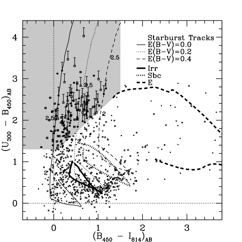
Figure 1: $(U_{300}-B_{450})_{AB}$/$(B_{450}-I_{814})_{AB}$ colour-colour diagram illustrating the position of our $U$-dropout sample (shaded region) relative to the photometric sample as a whole. Tracks for a $10^{9}$ year starburst with various amounts of extinctions have been included to illustrate both the typical redshifts and SED types included in the selection window. The low-redshift ($0<z<1.2$) tracks for typical E, Sbc, and Irr spectra have been included as well to illustrate the region in colour-colour space where possible contaminants might lie. Solid (open) squares indicate objects from the HDF North (HDF South). Larger squares indicate objects found in our sample. Error bars represent 1.5 $\sigma$ limits.

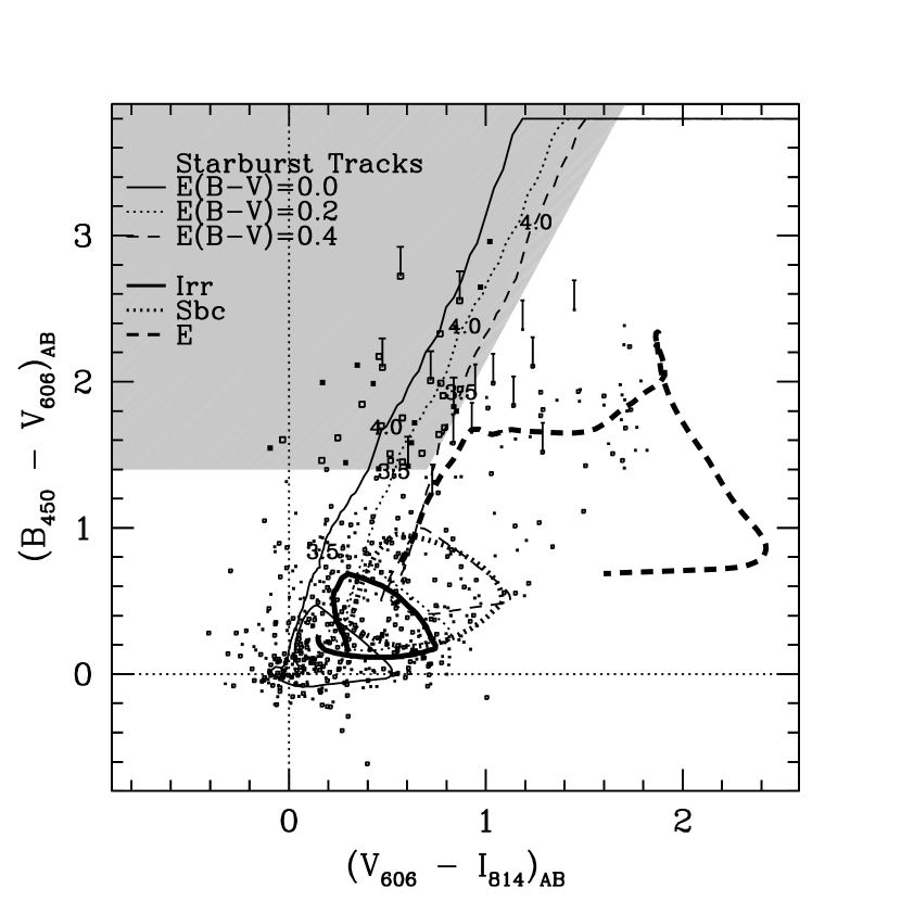
Figure 2: $(B_{450}-V_{606})_{AB}$/$(V_{606}-I_{814})_{AB}$ colour-colour diagram illustrating the position of our $B$-dropout sample (shaded region) relative to the photometric sample as a whole. Otherwise the same as Figure 1.

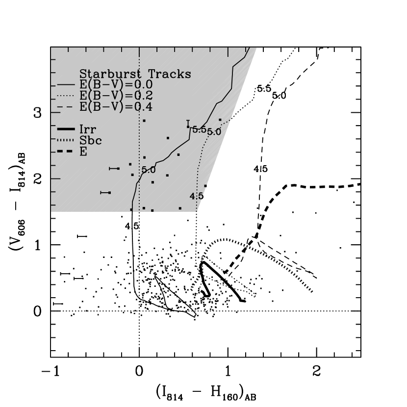
Figure 3: $(V_{606}-I_{814})_{AB}$/$(I_{814}-H_{160})_{AB}$ colour-colour diagram illustrating the position of our $V$-dropout sample (shaded region) relative to the photometric sample as a whole. Otherwise the same as Figure 1.

Due to the small number of objects ($\sim 19$) in the above $V$-dropout sample, we consider an alternative $V$-dropout sample, with very red $(V_{606}-I_{814})_{AB}>1.8$ colors and no requirement on the optical-to-near-infrared color. This enables us to include the HDF South data where no deep space-based near-infrared images exist. While one might worry about the presence of lower redshift contaminants like EROs (Extremely Red Objects) in such a sample, the spectral slope redward of the break (e.g., the $(I_{814}-H_{160})_{AB}$ color) for similarly red objects in the HDF North tends to be relatively flat, indicating that most faint red objects are indeed at high-z ($z\sim 4-6$), and so the contamination is not very large. We call this sample the optical $V$-dropout sample (“V-dropout (Opt)”) to distinguish it from the $V$-dropout sample described in the previous paragraph where infrared fluxes are used (“V-dropout (IR)”).

We have made sure to set up the selection criteria so that the intrinsic set of objects selected by either our $B$ dropout criterion or our $V$ dropout criterion–as parametrized by absolute magnitude or spectral index–are subsets of those selected by our $U$ dropout criterion. This is important whenever one projects one sample onto another for the sake of intercomparison: one needs to insure that the set of galaxies into which one is mapping, i.e., the range, is strictly a subset of the galaxies one is mapping, i.e., the domain. Otherwise, one can not preclude there being some population of galaxies in the range (e.g., the mapped-into sample) which do not have duplicates in the domain (the mapped sample). In the present case, this would mean making the mistake of comparing a $U$-dropout sample, defined to include only the bluest U-dropouts ($E(B-V)<0.1$), with $B$ and $V$-dropout samples, defined to include all ranges of intrinsic $E(B-V)$ reddenings, by projecting the former onto the latter. The selection criteria given above were chosen to avoid these type of difficulties.

3 Results

3.1 Derived Samples

Using the photometry and sample selection procedure described in Appendix A, we found 61 and 72 $U$-dropouts for the HDF North and South, respectively. We found 15 and 21 $B$-dropouts for the HDF North and South, respectively. Finally, we found 19 $V$-dropouts for the HDF North. We also found 12 and 6 objects in the HDF North and South, respectively, with very red $(V_{606}-I_{814})_{[AB}>1.8)$ colors. We determined the object redshifts photometrically, or spectroscopically if available, and determined the SED templates that best-fit their pixel-by-pixel fluxes. Spectroscopic redshifts are available for 17 objects from our $U$-dropout sample and are in excellent agreement with our photometric redshift estimates (see Figure 4), the overall RMS scatter $\sqrt{\left\langle\left[(\Delta z)/(1+z)\right]^{2}\right\rangle}$ being only 0.05. This being said, the photometric redshifts do seem to have a small upward bias in redshift compared to the spectroscopic measures, e.g., $\left\langle(\Delta z)/(1+z)\right\rangle=0.02$. This small bias does not appear to be a big problem because we were able to independently replicate all our results (within $\sim 10-15$%) using the Steidel et al. (1999) $z\sim 3$ luminosity function. We remark on this briefly at the end of §4. Figure 5 contrasts the intrinsic SED distribution we derive with that of Steidel et al. (1999). As detailed in Appendix A, the intrinsic SED be parametrized in terms of $E(B-V)$ by applying various amounts of extinction to some base spectrum. Clearly, our intrinsic SEDs are slightly bluer than those of Steidel et al. (1998). While this might well indicate slight differences in the exact shape of the SED templates and possible redshift biases, they don’t result in any large systematics. We comment on this later in §4. Finally, we provide basic plots of the number counts and angular size (half-light radii) distributions we obtained for these samples in Figure 6-10.

Figure 4: The upper panel compares the photometric redshifts we estimate for the $U$-dropouts with the spectroscopic values. The scatter is small, $\sqrt{\left\langle\left[(\Delta z)/(1+z)\right]^{2}\right\rangle}=0.05$. There is a small upward bias in redshift compared to the spectroscopic measures, e.g., $\left\langle(\Delta z)/(1+z)\right\rangle=0.02$, but this is not an issue because we were able to independently replicate all our results (within $\sim 10-15$%) using the Steidel et al. (1999) $z\sim 3$ luminosity function (§4).

Figure 5: Comparison of the $E(B-V)$ distribution recovered for our $U$-dropout sample (histogram) with Steidel et al.’s (1999) determination (line) (see Figure 6 from that paper.) The relative normalization is set so as to allow comparison between Steidel’s sample and our HDF objects. The offset does not appear to be significant, particularly because we are able to reproduce all the latter results using both the $E(B-V)$ distribution shown above and the Steidel et al. (1999) luminosity function (§4). Negative values of $E(B-V)$ are used here for similarity with Steidel et al. (1999) since they provide a convenient way of representing templates bluer than our base spectral template.

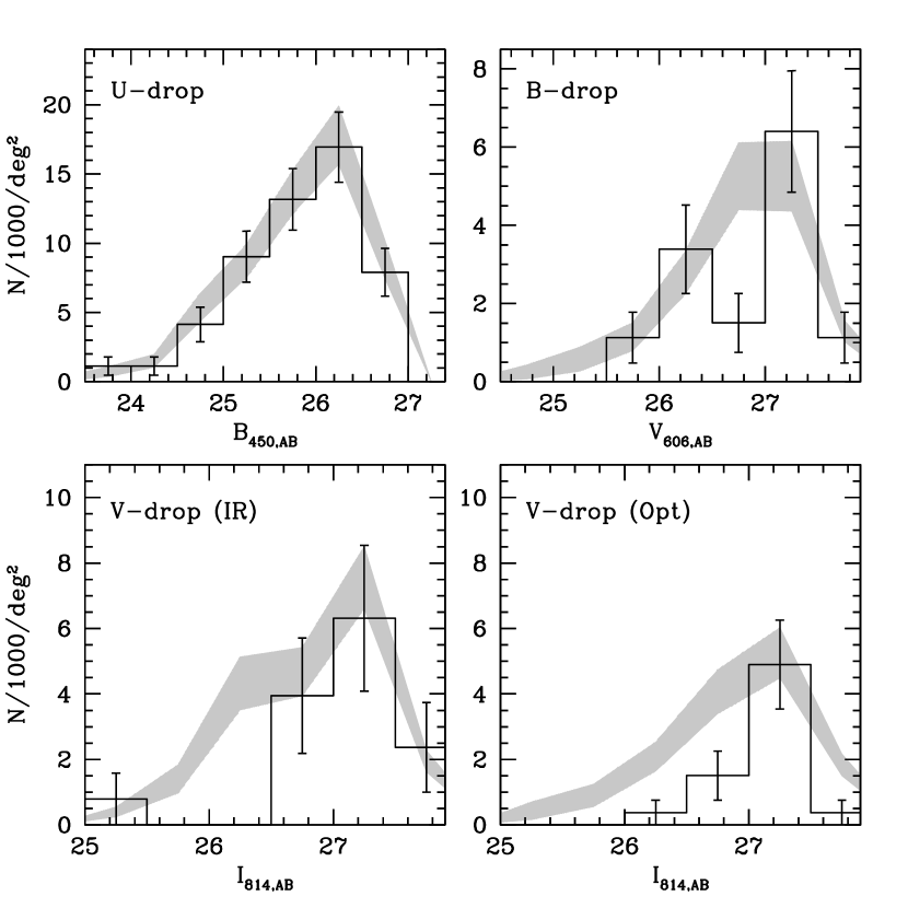
Figure 6: Comparison of the number counts for the $U_{300}$, $B_{450}$, and $V_{606}$ dropouts observed in the HDF (histogram) with the no-evolution expectations based upon our $U$-dropout sample (shaded regions). Definitions of all the dropout samples, including the two $V$-dropout samples are given in §2. Note the good agreement between the distribution recovered from the $U$-dropout samples (in the upper-left panel) and the cloning simulations derived from them (see §3.4).

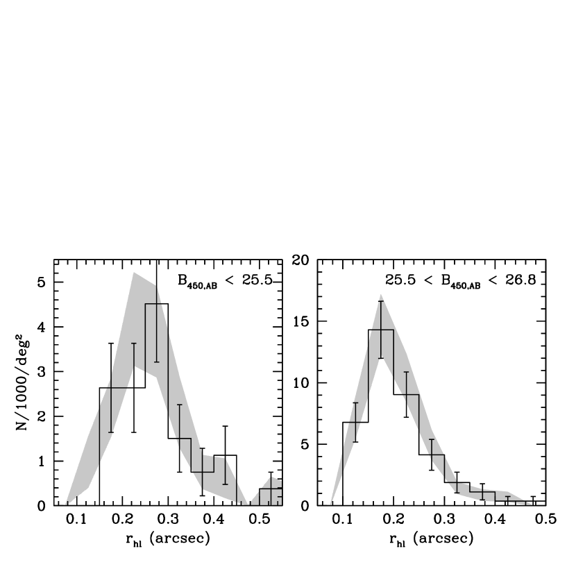
Figure 7: Comparison of the half-light radius distributions for the $U_{300}$ dropout sample with the cloning simulations derived from them for two different magnitude intervals using the $\Omega_{M}=0.3$, $\Omega_{\Lambda}=0.7$ geometry. Excellent agreement between the simulations and observations points toward a general self-consistency in our procedure (§3.4).

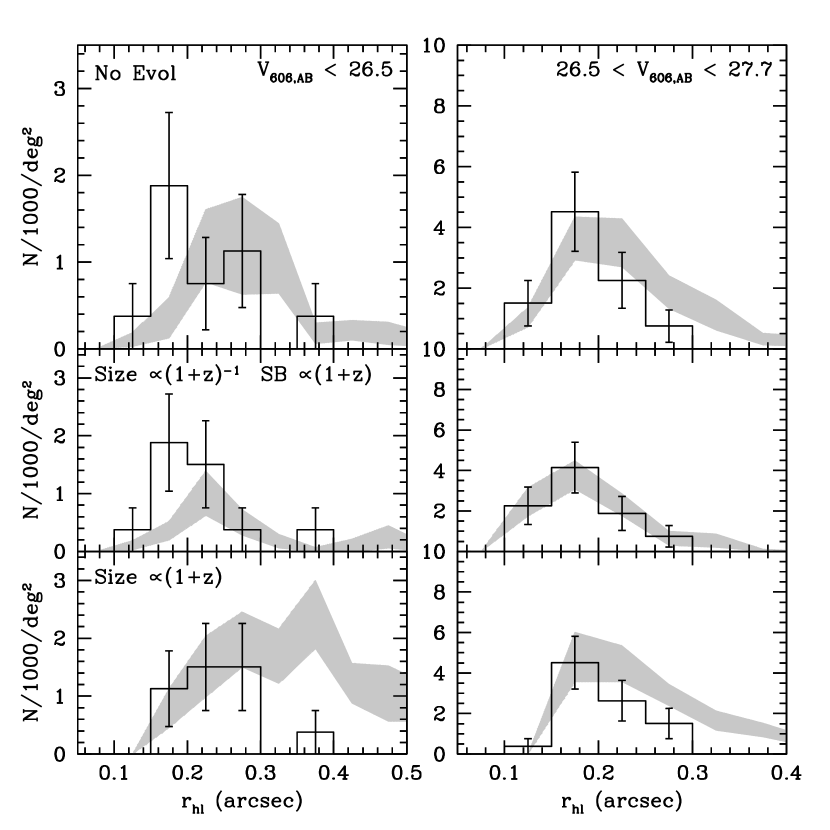
Figure 8: Similar to Figure 7, but for the $B_{450}$-dropouts. The shaded regions indicate the expected values based upon the $U$-dropout sample. The predictions of a no-evolution model are presented in the top panel, those for our preferred size-evolution model with mild surface brightness evolution where size scales as $(1+z)^{-1}$ are presented in the middle panel, and those of a constant surface brightness size evolution model where sizes scale as $(1+z)$ are given in the bottom panel. In both magnitude intervals, the observed angular size distribution is somewhat smaller than that based upon a no-evolution projection of the $U$-dropout population. Note that because the effective PSF of our $z\sim 2-3$ templates is typically larger than for the observations at $z\sim 4$ (see §3.3 for a more detailed explanation), it is necessary for us to apply varying amounts of smoothing to the observations before making a comparison with the lower redshift population.

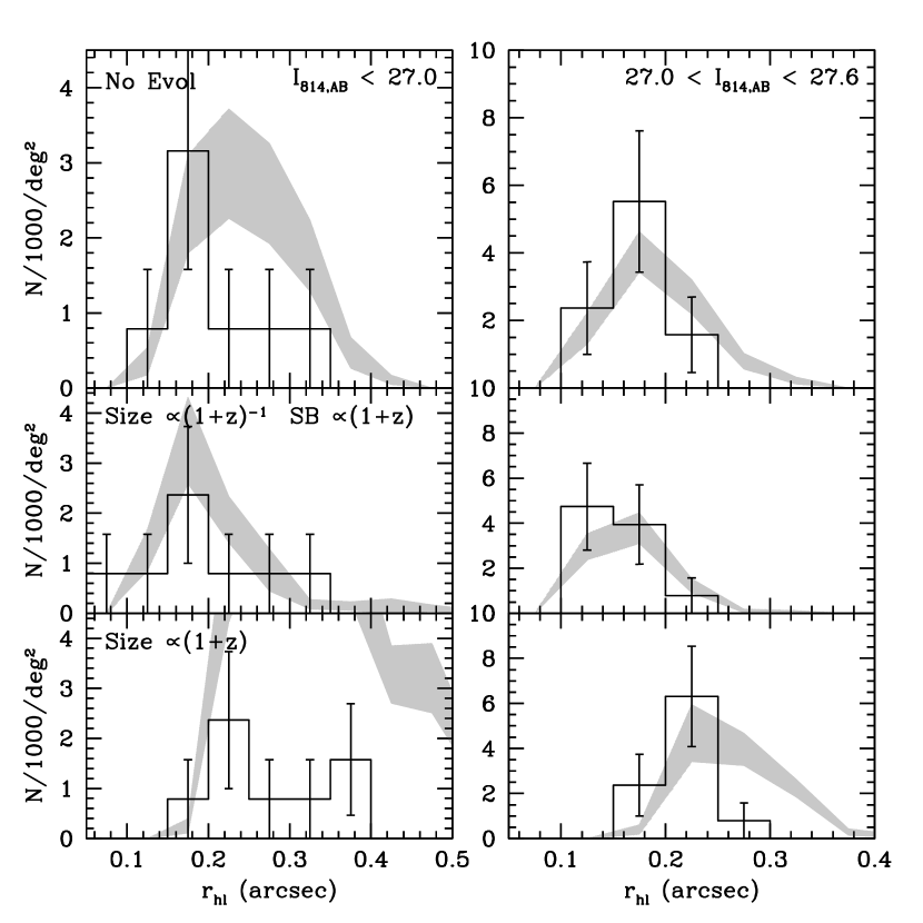
Figure 9: Similar to Figure 8, but for $V_{606}$-dropouts selected using the infrared photometry (“V-drop (IR)”). The observed angular size distribution of the bright slice ($I_{814,AB}<27$) (histogram) are smaller (90% confidence) than that predicted based on the $U$-dropout sample ($z\sim 2.7$) (top panel), the $(1+z)^{-1}$ model shown in the middle panel providing the best-fit to the size evolution observed. Together with Figure 10, this shows that $UV$ bright objects are smaller at $z\sim 5$ than at $z\sim 2.7$.

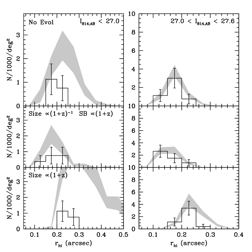
Figure 10: Similar to Figure 9, but for the “optical” $V_{606}$-dropouts selected from the HDF North and South. The fact that the observed angular size distribution (histogram) for the bright slice ($I_{814,AB}<27$) is shifted toward smaller sizes than that predicted from the $z\sim 2.7$ $U$-dropouts clearly suggests that galaxies are smaller at $z\sim 5$ than at $z\sim 2.7$ (86% confidence). Together with Figure 9, this shows that galaxies are smaller at $z\sim 5$ than they are at $z\sim 2.7$. In both, the best fit is provided by the middle panel with a $(1+z)^{-1}$ scaling in size.

We determined the volume densities of each object in these base samples using the procedure given in Appendix C. Briefly, we projected the galaxy to all redshifts using the procedure described in Appendix B, remeasured its properties, and then took its volume density to be the reciprocal of the effective selection volume. Using the volume densities determined in Appendix C, it was straightforward to derive an estimated luminosity function for both the $U$ and $B$-dropouts. Note that we determined $M_{1700,AB}$ magnitudes using each object’s $I_{814}$ magnitude and best-fit pixel-by-pixel SED. We include these LFs on Figure 11 in the form of solid and open boxes for the $U$ and $B$-dropouts, respectively, the error bars representing one-sigma uncertainties. We also include various results by Steidel et al. (1999) on that plot, but will also leave a discussion of that until later (§5.2). While the $U$-dropout LF has a normalization which is roughly $2\times$ higher than the $B$-dropout LF, we will argue that the intrinsic normalizations are closer than this and the apparent difference is largely a consequence of the differing selection effects (§5.2).

Figure 11: Rest-frame ($z=3$) luminosity functions for the U-dropout sample (filled squares) and the B-dropout sample (open squares) used in the present study assuming a $\Omega_{M}=0.3$, $\Omega_{\Lambda}=0.7$ geometry and $H_{0}=70\,\textrm{km/s/Mpc}$. Note that the faintest two bins in our LFs suffer from incompleteness. Our LF matches Steidel et al.’s (1999) LF at $z\sim 3$ (filled circles; thick solid line), but falls below their determination at $z\sim 4$ (open circles; thick dotted line). The Pozzetti et al. (1998) LF at $z\sim 3$ (thin solid line) and at $z\sim 4$ (thin dotted line) are also shown.

3.2 Sample Fairness

It is useful to assess the fairness of our samples, especially given the surprising amount of clustering observed at high redshift (Steidel et al. 1998; Giavalisco et al. 1998; Adelberger et al. 1998) and possible systematics in the photometric redshifts we use. To this end, we plot $V/V_{max}$ (Schmidt 1968) for our $U$ dropout sample in Figure 12. For a homogeneous sample in magnitude and redshift, the quantity $<V/V_{max}>$ should equal

$$0.5\pm\frac{1}{\sqrt{12N}}$$

where $N$ is the number of the galaxies in the sample ($N=142$). Our samples meet this goal, and even more encouragingly, we find that the $V/V_{max}$ distributions are relatively flat.

Figure 12: $V/V_{max}$ distribution for the $U$ dropout samples for the $\Omega_{M}=0.3$, $\Omega_{\Lambda}=0.7$ geometry. The horizontal line shows the expected value for each bin. The error bars show the expected one sigma variations in the expected numbers. The fact that the $V/V_{max}$ distribution is flat and here agreement shows that our $U$ dropout sample is fair.

3.3 Simulating the $U$, $B$, and $V$ Dropout Samples

It is now completely straightforward to use the number densities derived to compare the $U$-dropout objects with all the other samples compiled here, including the $U$ dropout sample itself. Assuming no spatial clustering, we use the cosmological volume and object volume densities to generate Monte-Carlo object catalogs over a given redshift interval and effective area of $2.5\times 10^{5}$ $\textrm{arcsec}^{2}$. We simulate the appearance of objects at new redshifts using the steps outlined in Appendix B.1-B.4, and we measure their properties using the techniques discussed in Appendix B.5. Applying the selection criteria relevant to the fiducial sample, we are able to compile the properties of the projected base sample. We compute one-sigma uncertainties on the expected numbers based upon the number of objects from our input samples which contribute to the inferred numbers. Our procedure for deriving error estimates is fully described in BBSI and is similar to what one would obtain from a bootstrapping analysis. In future sections, we often refer to this as our empirical $U$-dropout model. It is used almost exclusively to make predictions. Before comparing our projected $U$-dropouts with higher redshift data, we smooth the data slightly so as to match the projected PSF of $z\sim 2-3$ objects at $z\sim 4-5$. This is necessary because the angular size, and therefore effective PSF, of objects is smaller at $z\sim 2-3$ ($\textrm{FWHM}_{PSF}\sim\,$0.14 arcsec) than it is when projected to $z\sim 3-6$ ($\textrm{FWHM}_{PSF}\sim\,$0.18 arcsec at $z\sim 5$) for the $\Omega_{M}=0.3$, $\Omega_{\Lambda}=0.7$ geometry.

3.4 Simulation Self-Consistency

Clearly, using the $U$-dropout clones, we should be able to make Monte-Carlo simulations of the high redshift universe and recover something similar to the $U$-dropout observations from which the empirical models were derived. In Figure 6, we show the observed number counts for the $U$-dropouts and overplot our cloning expectations based upon this same $U$-dropout sample. The shaded regions show the variation expected due to the finite size of our input samples. In Figure 7, we do the same for the angular sizes of the $U$ dropouts, the histogram indicating the observations and the shaded regions indicating that expected from cloning the $U$ dropouts. In all cases, the $U$-dropout samples successfully reproduce the parent distributions from which they were derived.

3.5 Number Counts

Comparing the observed number counts with those predicted from our empirical $U$-dropout model allows us to test the extent to which the luminosity, size, and colour distributions of $UV$-bright galaxies change as a function of redshift. First, we consider basic number count predictions. Figure 6 shows how the observed $B$ and $V$-dropout number counts compare with those predicted based upon the $U$ dropout samples (shaded region). Clearly, we expect more $B$ and $V$ dropouts based upon the cloned $U$-dropout population than are actually observed in the HDF fields. Integrating down the number counts, one infers there are 40% less $UV$-bright galaxies at $z\sim 4$ than there are at $z\sim 2.7$ and $\sim 46$% less at $z\sim 5$ than at $z\sim 2.7$. Obviously, these numbers are slightly different than those we gave earlier (§3.1) in comparing the luminosity functions over this same redshift range, and the reason isn’t that surprising: the $U$-dropout selection criterion includes objects which aren’t included in the $B$-dropout criterion, specifically objects of lower surface brightness and redder colors. We will discuss these differences a little more extensively later (§5.2).

3.6 Galaxy Sizes

Next, we proceed to an examination of the angular sizes. This is important because it provides crucial new information on the extent to which galaxies may have evolved in size from $z\sim 5$ to $z\sim 2.7$, not discernible using ground-based data. Figures 7-10 present the angular size (half-light radii) distributions for the $U$, $B$, $V$-dropout samples along with a comparison with the predicted distribution based upon the $U$-dropout population (shaded regions). Stepping from $z\sim 2.7$ to $z\sim 4$, a clear size difference is already apparent, particularly in the brightest magnitude bin ($V_{606,AB}<26.5$). This size difference becomes even more obvious when the comparison is made at $z\sim 5$ (both for the optical and infrared $V$-dropout samples), this difference again being the largest in the brightest magnitude bin ($I_{814,AB}<27$). We illustrate this difference more graphically by showing a random sample of the observed $B$-dropouts and those predicted based upon the $U$-dropout population in Figure 13. We do a similar thing for the $V$-dropouts in Figure 14. Clearly, the observed $V$-dropouts are slightly smaller on average and more centrally concentrated in surface brightness.

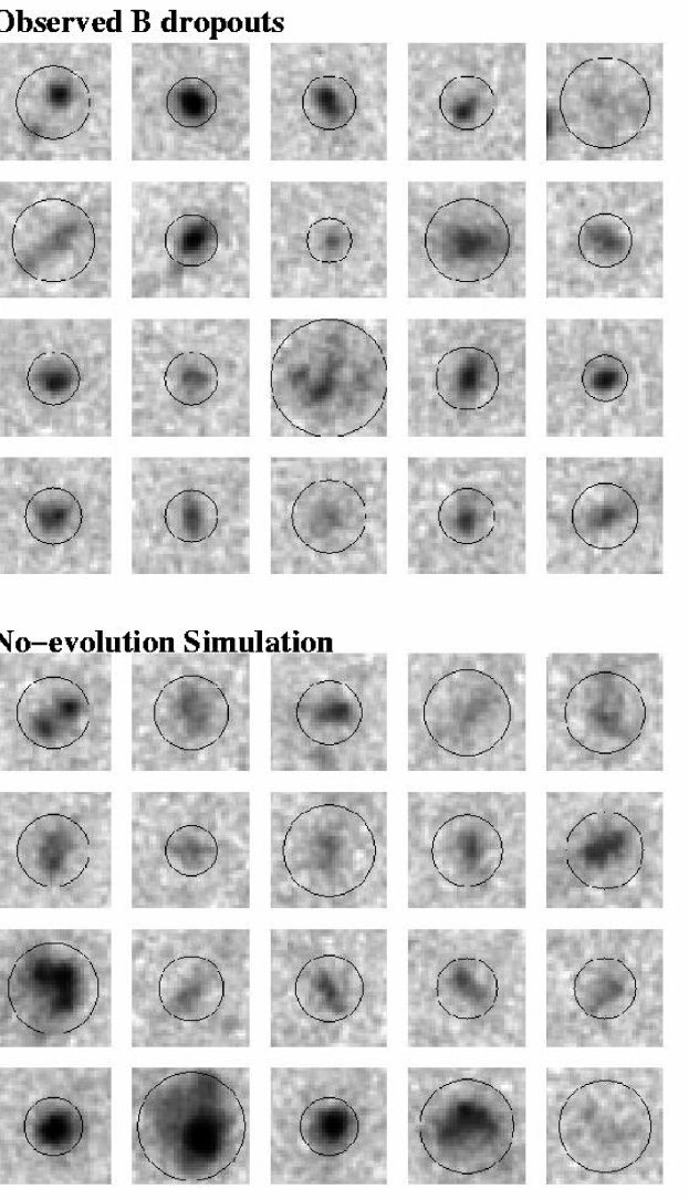
Figure 13: Postage stamp images of the $B$-dropouts ($z\sim 4$) identified in the HDF North and South (upper panel) versus those expected from a no-evolution extrapolation of our $z\sim 2.7$ $U$-dropout sample (lower panel). Circles demarking twice the determined half-light radius are included for each object. As demonstrated quantitatively in Figure 8, the mean size of the observed $B$-dropout population is smaller than that predicted based on a no-evolution extrapolation from the $U$-dropout population and is quite evident from a comparison of these panels (from the mean size of the half-light distributions). Plate scale is 1.36 arcsec.

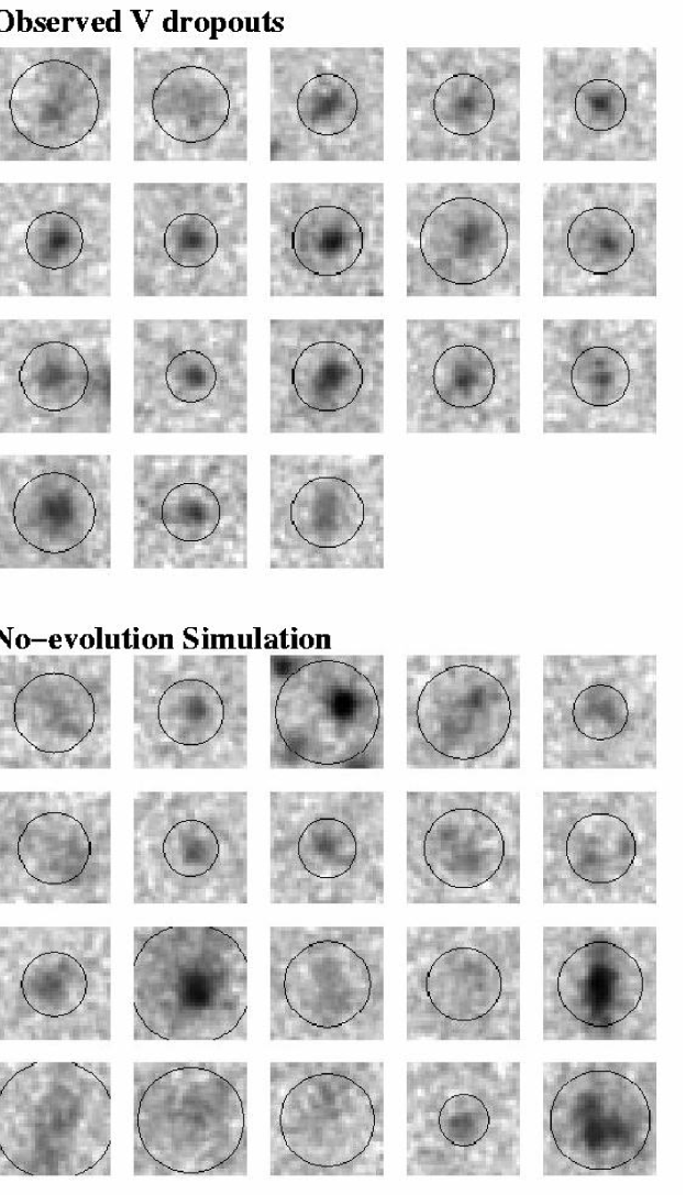
Figure 14: Postage stamp images of the $V$-dropouts ($z\sim 5$) identified in the HDF North and South (upper panel) versus those expected from a no-evolution extrapolation of our $z\sim 2.7$ $U$-dropout sample (lower panel). All 18 “optical” $V_{606}$ dropouts are shown. Circles demarking twice the determined half-light radius are included for each object, as in Figure 13. As demonstrated quantitatively in Figure 9 and Figure 10, the mean size of the observed $V$-dropout population is smaller than that predicted based on a no-evolution extrapolation from the $U$-dropout population with evidence that the mean surface brightness has evolved too. Plate scale is 1.36 arcsec.

To examine the rate of evolution in size we repeated the experiment of cloning the $U$-dropout population to higher redshift but scaled the sizes by $(1+z)$ (solid lines) without changing the surface brightnesses. We also considered the case where the size scaled as $(1+z)^{-1}$ and the surface brightness varied as $(1+z)$ (dashed lines). These lines are presented both in comparison with the $B$-dropouts (Figure 8) and the $V$-dropouts (Figures 9-10). As might be expected, the constant surface-brightness size-evolution model where size $\propto$ $(1+z)$ overestimates both the sizes and numbers considerably. Our other size-evolution model (where sizes decrease as a function of redshift), however, fares much better, providing a decent fit to the observations, suggesting that galaxies are $(1+5)/(1+2.7)\sim 1.7$ times larger at $z\sim 2.7$ than they are at $z\sim 5$.

It is also instructive to take the angular size distributions of the $U$, $B$, and $V$ dropouts shown in Figure 7, Figure 8, and Figure 10 (we take the brighter magnitude slices) and represent them in terms of their intrinsic physical size, assuming they lie at $z\sim 2.7$, $z\sim 4$, and $z\sim 5$ (Figure 15). We perform a similar scaling to the different projections of our $U$-dropout populations shown on Figures 7, 8, and 10. It is evident that while the physical sizes of the $V$-dropout population are significantly smaller than the $U$-dropouts for all geometries, the extrapolated $U$-dropout population are also much smaller given the $B$ and $V$ selection criteria. Obviously, this latter shift toward smaller intrinsic sizes must arise from the selection procedure itself and cannot be due to evolution. Therefore, the apparent evolution in the size of UV-bright population can only be partially an issue of evolution. This illustrates how important a consideration of selection effects are for the present analysis.

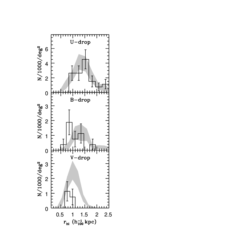
Figure 15: A comparison of the physical sizes of the bright $U$-dropouts ($B_{450,AB}<25.5$), $B$-dropouts ($V_{606,AB}<26.5$), and $V$-dropouts ($I_{814,AB}<27.0$) (histograms) with the sizes recovered from the extrapolated $U$-dropout population (shaded regions) for the $\Omega_{M}=0.3$, $\Omega_{\Lambda}=0.7$ geometry. While the physical size of the $V$-dropouts is clearly smaller than the $U$-dropouts (compare the histograms in the top and bottom panels), the projected $U$-dropouts (via no-evolution) also tend to be much smaller because of the selection effects, so the apparent evolution in the size of the $UV$-bright population is only partially an issue of evolution. This demonstrates how important a consideration of selection effects can be for measuring evolution.

We now attempt to determine the statistical significance of our finding that galaxies at $z\sim 3$ seem to be larger than those at $z\sim 5$. To this end, we shall suppose that both samples can be approximated by a normal distribution and we shall test the null hypothesis that the mean of one sample (our projected $z\sim 3$ sample) is larger than the mean of the other (our observed $z\sim 5$ sample.) Formally, we use the T test:

$$T=\frac{\bar{X}_{1}-\bar{X}_{2}}{\sigma\sqrt{\frac{1}{n_{1}}+\frac{1}{n_{2}}}}$$ (1)

where

$$\sigma=\sqrt{\frac{n_{1}S_{1}^{2}+n_{2}S_{2}^{2}}{n_{1}+n_{2}-2}},$$ (2)

where $\bar{X}_{i}$ is the mean for sample $i$, $S_{i}$ is the variance for sample $i$, $n_{i}$ are the number of objects in sample $i$ (e.g., Hogg & Tanis 1993). We derive T = 1.64 and T = 1.49 for the brighter ($I_{814,AB}<27$) objects in Figures 9 and 10, respectively. This works out to a 90% confidence and 86% confidence result, respectively, providing suggestive evidence that $UV$-bright galaxies are smaller at $z\sim 5$ than they are at $z\sim 3$.

3.7 Colour Distributions

We now look at how the colours of the $B$ and $V$-dropout populations compare with that expected based upon lower redshift populations to examine the evolution of intrinsic colours. Figure 16 compares the observed color distribution of the $U$, $B$, and $V$ dropout samples (histogram) with that expected from the $U$-dropout population (shaded region). The color distribution at $z\sim 4$ and $z\sim 5$ seems to have a very similar shape to that predicted based upon the lower redshift sample, at $z\sim 5$ suggesting that there hasn’t been a lot of evolution in the intrinsic age, metallicity, or dust content of high redshift galaxies over this redshift interval.

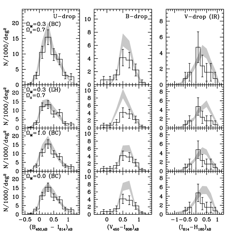
Figure 16: A comparison of the simulated (shaded regions) and observed (histogram) colour distributions for the $U$, $B$, and $V$-dropout samples. The shaded regions represent no-evolution expectations based on our $U$-dropout sample. We provide the canonical results based on the $\Omega_{M}=0.3$, $\Omega_{\Lambda}=0.7$ geometry and BC spectral template set in the top panel. We also include results using the LH spectral template set, the $\Omega_{M}=1$ geometry, and $\Omega_{M}=0$ geometry in the lower panels to illustrate possible model dependencies. The distribution of intrinsic colors appears to show minimal evolution from $z\sim 5$ to $z\sim 3$, suggesting similarly small changes in the age, metal, or dust-content of this $UV$-bright population.

3.8 Redshift Distributions

To illustrate the redshift distributions for the objects in our dropout samples and to comment on the selection windows used for these purposes, we compare our estimated redshift distributions (histogram) with those predicted by extrapolating our $U$-dropout population to higher redshift (shaded regions). The redshift distribution for the $U$, $B$ and $V$-dropouts agree quite well with that expected based upon the $U$-dropout population. Note that for both the $U$ and $B$-dropout samples we observe a downturn at lower redshift than suggested by Figure 17 of Steidel et al. (1999). This results because the redder band used in defining the spectral break no longer has sufficient signal-to-noise at higher redshift to make a strong constraint on the color. Consequently, one finds that real objects make “inverted-V” shapes as they track through colour-colour space. They therefore tend to drop out of the selection window at lower redshifts than one might naively expect if the object had infinite signal-to-noise in both passbands defining the spectral break. This is illustrated in Figure 18 for 3 objects from our $U$-dropout sample. The tracks they make in colour-colour space assuming infinite S/N are also shown (solid line).

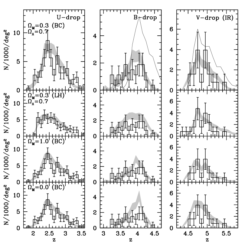
Figure 17: Comparison of the simulated (shaded regions) and observed (histogram) redshift distributions for the $U$, $B$, and $V$-dropout samples. The shaded regions represent the no-evolution expectations based on our $U$-dropout sample. Note the good agreement between the predicted $U$-dropout redshift distributions and the observed ones. The thin solid lines represent the redshift distribution predicted with no observational errors. Note that this latter distribution is higher in both number and redshift than is actually obtained when observational errors are included, demonstrating the importance of including such effects.

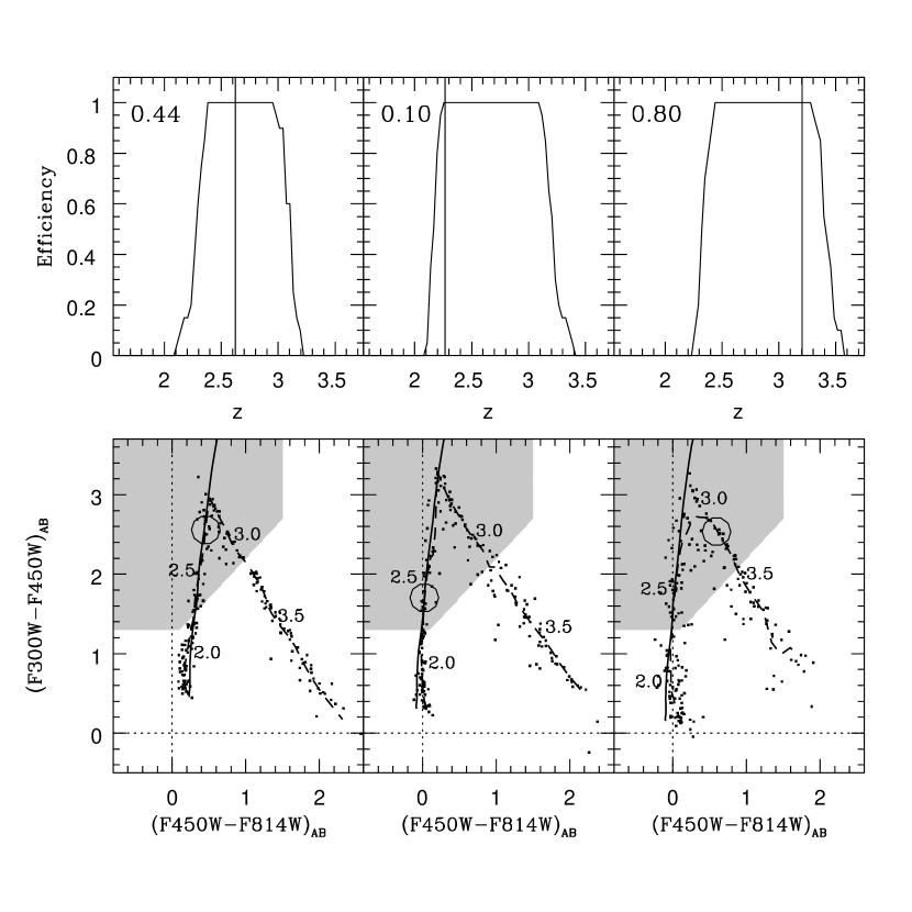
Figure 18: The upper panels show typical determinations of the redshift selection efficiencies $\epsilon(z)$ for three $U$-dropout galaxies. Each panel also includes a vertical line at the estimated redshift and the corresponding $V/V_{max}$ (upper left-hand corner of each panel). The lower panels illustrate the Monte-Carlo simulations we perform to see how the photometry of each object (dots) tracks across redshift space, specific redshifts being annotated there. The solid and dashed lines indicate how the object tracks in color-color space given infinite and the observed signal-to-noise, respectively. (The shaded region denotes the $U$-dropout selection window.) The actual colors for each object are indicated by the large circles.

To illustrate the effect this has on the selection window, we repeat our extrapolation of the $U$-dropout population to higher redshifts (§3.3), but now assume that the object colours simply derive from their best-fit spectral types. We include this as thin solid lines in all panels on Figure 17. Clearly, many more galaxies are expected to be selected at high redshift using this method than one finds by resimulating the object at higher redshift and recovering its parameters there. This effect, among other things, may have led others to overestimate the dropoff in luminosity density from $z\sim 3$ to $z\sim 4$ based on the HDFs. This underlines the importance of doing detailed simulations to understand the selection effects at work in estimating evolution across a sample.

3.9 Star Formation History

We now look at the evolution of the luminosity density. Typically, this has been calculated by (1) determining the luminosity function for a high redshift population, (2) determining the total luminosity density by integrating along the luminosity function, and (3) converting the observed luminosity density to a star formation rate density using some prescription. Unfortunately, this method suffers when the implicit set of galaxies selected varies as a function of redshift.

Here, we proceed as follows. For the $U$-dropouts, we determine the luminosity density in the standard way described above, but for the $B$ and $V$-dropouts, we determine the luminosity densities differentially, namely, by comparing the observed dropout counts with that expected from a no-evolution projection of the $U$-dropout population to higher redshift. Otherwise stated, we take the luminosity density of the $U$-dropouts to be

$$L_{UV}(U)=L_{UV}(Obs,U),$$ (3)

the luminosity density of the $B$-dropouts to be

$$L_{UV}(B)=L_{UV}(Obs,U)(\frac{L_{UV}(Obs,B)}{L_{UV}(Sim,U\mapsto B)}),$$ (4)

and the luminosity density of the $V$-dropouts to be

$$L_{UV}(V)=L_{UV}(Obs,U)(\frac{L_{UV}(Obs,V)}{L_{UV}(Sim,U\mapsto V)}),$$ (5)

where $L_{UV}(Obs,U)$ is the integrated UV luminosity of the observed $U$ dropouts and where $L_{UV}(Sim,U\mapsto B)$ is the integrated UV luminosity of the $B$-dropouts recovered from projecting the $U$-dropout population to higher redshift. Note that the ratio $\frac{L_{UV}(Obs,B)}{L_{UV}(Sim,U\mapsto B)}$ is determined by summing the light found in the observed number counts and comparing that with the number predicted for our empirical $U$-dropout model. As remarked in §3.5, this works out to a measured $UV$-luminosity density which is 40% lower at $z\sim 4$ than it is at $z\sim 2.7$ and 46% lower at $z\sim 5$ than it is at $z\sim 2.7$. On the other hand, if we had simply determined the luminosity densities at $z\sim 4$ and $z\sim 5$ from the luminosity functions estimated there instead of differentially as we have done here, the shortfall would have been 60% and 71%, respectively.

We converted our derived luminosity densities to star formation rate densities using the relation

$$L_{UV}=\textrm{const}\,\,\textrm{x}\,\,\frac{\textrm{SFR}}{M_{\odot}\textrm{yr}^{-1}}\textrm{ergs}\,\textrm{s}^{-1}\,\textrm{Hz}^{-1}$$ (6)

where const = ($8.0\times 10^{27}$, $7.9\times 10^{27}$) at (1500 $\AA$, 2800 $\AA$) for a Salpeter IMF (Madau et al. 1998). Figure 19 illustrates the present results in the context of other typically cited determinations of the star formation rate density.

Figure 19: A history of the star formation rate density assuming no extinction correction. The determinations from this work (large solid circles) are in fair agreement with the previous high redshift determinations of Madau et al. (1998) (open circles), Steidel et al. (1999) (crosses), and Thompson et al. (2000) (filled triangles). The determinations from Lilly et al. (1996) (open squares) and Connolly et al. (1997) (solid squares) are shown for context. A Salpeter (1955) IMF is used to convert the luminosity density into a star formation rate (see, for example, Madau et al. 1998). Values are for a $\Omega_{M}=0.3$, $\Omega_{\Lambda}=0.7$ geometry and $H_{0}=70\,\textrm{km/s/Mpc}$. No correction is made for dust.

4 Possible Dependencies

All the results we have presented thusfar assume a $\Omega_{M}=0.3$, $\Omega_{\Lambda}=0.7$ geometry and utilize the BC spectral templates to perform the $k$-corrections. Here we repeat the entire analysis we performed in previous sections, but use different cosmologies and spectral templates to move the $U$-dropout galaxies through redshift space. In particular, we consider the $\Omega_{M}=0$ and $\Omega_{M}=1$ geometries; and for spectral template sets, we consider the Leitherer & Heckman (1995) model for a $10^{7}$ yr burst and metallicity $0.2Z_{\odot}$ with various amounts of dust reddening, this template set hereafter abbreviated as LH.

In Figures 20-21, we illustrate the effect that different cosmologies or spectral types have on the size distribution of the $B$ and $V$-dropouts predicted based upon the $U$-dropouts, respectively. Note that we smoothed the observed size distribution by different amounts to mimic the larger effective PSF of objects at $z\sim 4-5$. For both sets of dropouts, similar angular sizes are predicted for the flat $\Omega_{M}=1$ geometry as for the standard $\Omega_{M}=0.3$, $\Omega_{L}=0.7$ geometry used earlier in the paper. For the open $\Omega_{M}=0$ geometry, however, the angular sizes are predicted to be smaller and thus in better agreement with the observed size distribution. For the $B$-dropout sample, the LH template-set predictions are $\sim 50$% higher than for the BC templates. This results because of the different way the two template sets track through colour-colour space, one template set having a consistently higher $B$-dropout selection volume relative to the $U$-dropout selection volume. For the $V$-dropouts, however, the LH template set produces very similar predictions to the BC template set.

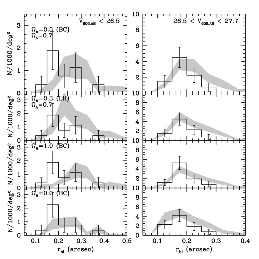
Figure 20: Similar to Figure 8, but using different geometries and spectral template sets to project the $U$-dropout sample to higher redshifts.

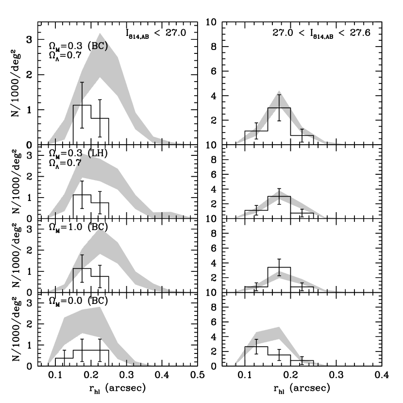
Figure 21: Similar to Figure 10, but using different geometries and spectral template sets to project the $U$-dropout sample to higher redshifts.

In Figures 16-17, we illustrate the effects of cosmology and template set on both the color and redshift distributions predicted based upon the $U$-dropouts. Clearly, there isn’t a large dependence on geometry, but the results do seem to depend a little on the spectral template set used, calculations involving the Leitherer & Heckman (1995) templates being slightly bluer and higher in normalization than those using the Bruzual & Charlot (1995) templates. The color differences are due to differences in the shape of the spectral templates–differences which also result in the LH template set having a consistently higher $B$-dropout selection volume than its $U$-dropout selection volume. A systematic study comparing real high redshift galaxy spectra to these spectral template sets might prove useful in eliminating these model dependencies. This, however, is beyond the scope of the present investigation.

We note here in passing that we checked our results by repeating all of our calculations assuming the Steidel et al. (1999) luminosity function, the Steidel et al. (1999) colour distribution, and real $U$-dropout profiles. The predictions we obtained were very similar (within $10-15$%) to those obtained by cloning the $U$-dropout population to higher redshift. This suggests that the redshift uncertainties present in our base sample do not have a large effect on our results.

5 Discussion

Up to this point analyses of differential evolution across high-redshift dropout populations have been restricted to luminosity functions (Pozzetti et al. 1998; Steidel et al. 1999), spatial clustering properties (Steidel et al. 1999; Giavalisco et al. 1998; Adelberger et al. 1998), and their colours (Steidel et al. 1999). Little work has been possible on the differential evolution of structural parameters.

5.1 Comparison with Casertano

It is instructive to compare our results with those of Casertano et al. (2000), who have also determined the number of $U$ and $B$ dropouts in the HDF North and South. Using nearly identical selection criteria, Casertano et al. (2001) found 68 $U$-dropouts in the HDF North compared to our 66, and 74 $U$-dropouts in the HDF South compared to our 76. For the $B$-dropouts and using a slightly more conservative selection criteria than ourselves, they found 11 dropouts in the HDF North compared to our 15, and 18 in the HDF South compared to our 21. Besides our use of different photometry, another reason for the slight differences between our results is that Casertano et al. (2000) do not exclude objects which are likely stars. Overall, though, our results agree quite well.

5.2 Luminosity Functions

We begin by comparing the luminosity functions we determined with previous determinations based on the HDFs, in particular those derived by Pozzetti et al. (1998) using the HDF North. We overplot their $U$-dropout ($z\sim 3$) and $B$-dropout ($z\sim 4$) luminosity functions on Figure 11 using thin solid and dotted lines, respectively. Before discussing a comparison of our derived LFs, let us remark briefly on their differences. The Pozzetti et al. (1998) study considers only the HDF North while we include the HDF South. The Pozzetti et al. (1998) study assumes that the selection volume for all $U$-dropout and $B$-dropout galaxies is uniformly $2<z<3.5$ and $3.5<z<4.5$, respectively, whereas we derive the selection volume for each galaxy individually, our estimated volume being 30-40% lower than the Pozzetti et al. (1998) estimate on average. The Pozzetti et al. (1998) study selects $U$-dropout galaxies in the $V_{606,AB}$ band while we select them in the $B_{450,AB}$ band. Finally, the Pozzetti et al. (1998) study uses the Kaplan-Meier (Lavalley, Isobe, & Feigelson 1992) estimators to determine the number of dropouts. In comparing our luminosity functions with those of Pozzetti et al. (1998), the bright end of our $U$-dropout LF is higher than the Pozzetti determination by about 70%, while the faint ends are more consistent. For the $B$-dropout LFs, our bright end also tends to be a bit higher in normalization while again at the faint end things are more consistent. Given the differences in our methodologies, we believe the differences are largely attributed to the different assumed selection volumes.

We now move into comparisons with the ground-based results of Steidel et al. (1998), for which there has been broad agreement at $z\sim 3$, but a more controversial discrepancy at $z\sim 4$ (Madau et al. 1996, 1997; Pozzetti et al. 1998; Steidel et al. 1999; Casertano 2000). Accordingly, it is not too surprising that the $U$-dropout luminosity function we derive at $z\sim 3$ (Figure 11) roughly agrees with those derived from Steidel et al. (1999). We include their $z\sim 3$ luminosity function as a set of solid circles and their fit as the thick solid line, where we take $M_{1700,AB}=-21.18$, $\alpha=-1.6$, and $\Phi=0.00198\,\textrm{Mpc}^{-3}$. Once again, at the bright end, our $U$-dropout luminosity tends to be a little high, but this is really quite understandable, especially considering that the scatter induced by photometric redshift uncertainties increases the number of galaxies at the bright end and decreases the number of galaxies at the faint end of the luminosity function.

Also, similar to other results on the HDFs, the $B$-dropout luminosity function we derive is clearly lower than that of Steidel et al. (1998). We include their $z\sim 4$ luminosity function as a set of open circles and the fit as a thick dotted line, where we take $M_{1700,AB}=-21.24$, $\alpha=-1.6$, and $\Phi=0.00154\,\textrm{Mpc}^{-3}$. While the same qualifications hold as for the derivation of the $U$-dropout luminosity function, the $B$-dropout luminosity function is some 60% lower in normalization than our $U$-dropout luminosity. Clearly, this is somewhat at odds with our finding in §3.9 that the $z\sim 4$ luminosity density is only 40% lower.

The only obvious way to rationalize these results is to conclude that there must be a class of objects which is selected at $z\sim 3$ by the $U$-dropout selection criteria and missed by the $B$-dropout criteria. Typically, the answer would be low luminosity galaxies, but a quick look at the luminosity functions (Figure 11) shows that this is not the answer, our $B$-dropout luminosity function probing fainter than its $U$-dropout equivalent. Instead, the difference seems to be more in the color cuts. Consider both Figure 2 of this paper and Figures 9-10 of Casertano et al. (2000). In both, we find significant numbers of modestly red galaxies barely excluded from both $B$-dropout samples (see the $E(B-V)\sim 0.3-0.4$ track in Figure 2), objects which are included in the $U$-dropout selection (Figure 1). Add to this the likely scenario that several of the lower surface-brightness $U$-dropout galaxies would tend to be missed in $B$-dropout samples due to the surface brightness dimming effects and it becomes quite apparent that there could be large differences in the derived luminosity functions without significant evolution in the underlying populations. This, in fact, is an excellent illustration of the difficulties inherent in measuring evolution from the luminosity function alone and why it is much better to infer evolution differentially as we have done here. The reason is simple: the cloning procedure outlined here automatically corrects for differences in the selection function in order to estimate evolution. To make similar estimates from a set of luminosity functions, one has to be sure that their selection functions are exactly the same. This latter task, quite obviously, is difficult to do cleanly and to the same surface brightness threshold. The preferred approach is clearly a differential one as used here.

5.3 Colour distributions

Steidel et al. (1999) used a model based upon their observationally-determined luminosity function and distribution of different dust-reddened spectral types to reproduce their ground-based $B$-dropout redshift distribution. As noted in this same work, this suggests that there hasn’t been a dramatic change in the distribution of UV-bright spectra from $z\sim 3$ to $z\sim 4$. We find a similar result to both $z\sim 4$ and $z\sim 5$, suggesting there has been minimal evolution in the age, metal, and dust-content content of $UV$-bright objects from $z\sim 3$ to $z\sim 5$. A priori little is known about colour evolution given the huge dependence on both the content and distribution of dust in these young star-forming objects.

5.4 Galaxy Sizes

At lower redshifts, there has already been a lot of observational work looking for possible size evolution. It is still somewhat controversial whether $L_{*}$ disk galaxies evolve in size from $z\sim 0$ to $z\sim 1$ (Lilly et al. 1998; Mao, Mo, & White 1998; Simard et al. 1999; Bouwens & Silk 2002; Bouwens et al. 2002). However, when low redshift galaxies are compared with fainter, higher redshift objects ($z>1-2$), there tends to be relatively consistent agreement that objects become smaller (BBSII; Roche et al. 1998; de Jong & Lacey 2000; Bouwens & Silk 2002; Bouwens et al. 2003).

In the high redshift interval ($z>2$) little to no observational work has been done on the differential evolution of galaxy sizes, despite the availability of high resolution HDF data. From a theoretical perspective, one expects the size of virialized objects to scale as $H(z)^{-2/3}$ for a fixed mass (e.g., Mo, Mao, & White 1998). This is simply derived from the scaling of the mean mass density with redshift, so that galaxies of a fixed mass interior to the virial radius must be denser at higher redshift.

For all cases but the completely open universe, the matter term $\Omega_{M}$ dominates at high redshift:

$$H(z)=H_{0}\sqrt{\Omega_{\Lambda}+(1-\Omega_{M}-\Omega_{\Lambda})(1+z)^{2}+\Omega_{M}(1+z)^{3}}.$$ (7)

More simply, for $\Omega_{M}=0.3$, $\Omega_{\Lambda}=0.7$ and $\Omega_{M}=1$, $H(z)\propto(1+z)^{3/2}$, and so the size of objects might be expected to scale as $(1+z)^{-1}$ with redshift. This is consistent with our observed $(1+z)^{-1}$ scaling. It is far from clear, however, that an appreciable fraction of the $UV$-bright objects at high redshift are found in virialized halos with rotationally cool disks. Most of them might well be merging gas clumps within halos that are just beginning to virialize.

5.5 Luminosity Density

The luminosity densities we derived from $z\sim 2.7$ to $z\sim 5$ tend to be consistent with previous findings (Madau et al. 1998; Thompson et al. 2001; Steidel et al. 2000) with the possible exception of the UV density at $z\sim 4$ where our estimates are modestly higher than previous estimates based on the HDFs, but we have already discussed those differences in §5.2. Overall, there is a clear trend towards lower luminosity densities at high redshift, our $z\sim 5$ sample being lower by some $\sim 46$%. Interestingly enough, this decrease is very similar to the expected $(1+z)^{-1}$ fall-off in sizes for our preferred model from §3.6: $(1+2.7)/(1+5)\sim 0.62$ or $\sim 38$%.

5.6 Comparison With Other Methods

This paper is part of a long-term effort to measure the differential evolution of galaxies from low redshift to high redshift. However, it is by no means the only attempt to make a systematic comparison of galaxy properties over such a large redshift range. More than for any other galaxy property, it has become fashionable to compile the UV luminosity function (or in its more popular form the star formation rate density) as a function of redshift (Madau et al. 1996, 1998; Connolly et al. 1997; Cowie et al. 1999; Yan et al. 1999; Steidel et al. 1999; Thompson et al. 2001). Unfortunately, the shear magnitude of cosmic surface brightness dimming at high redshift makes the process of comparing high-redshift galaxy populations with low redshift ones quite difficult. Specifically, a large population of disk galaxies could exist at $z\sim 3-4$, contribute a significant amount to the $UV$ luminosity function and cosmic star formation rate density, and remain entirely undetected given the amount of surface brightness dimming.

Lanzetta et al. (2001) has attempted to address this problem by examining the cosmic star formation intensity distribution, where a star formation rate density is assigned to each pixel instead of to each object. By looking at the distribution of UV surface brightnesses instead of the total luminosities, it is relatively straightforward to compare galaxy populations at a variety of redshifts and to apply the appropriate cuts in surface brightness. Thompson et al. (2001) follow Lanzetta et al. (2001) in use of this approach.

While we are encouraged by the attention such approaches give to important selection effects such as cosmic surface brightness dimming, we do not favor this approach for a number of reasons. First, Lanzetta et al. (2001) use photometric redshifts to divide their galaxies into different redshift samples. While photometric redshifts produce very accurate results for a good fraction of objects in the HDF at low and high redshift, there are still many objects with redshift degeneracies, i.e., two very different redshifts which are equally likely, and it is not generally clear that low redshift objects are not contaminating high redshift samples and high redshift objects low redshift samples. This is especially problematic if one uses a simple maximum likelihood approach since it is functionally equivalent to using a flat prior in redshift, a prior which effectively assumes that $L_{*}\propto D_{L}(z)^{2}$. Therefore, one should not be too surprised that Lanzetta et al. (2001) find a monotonically increasing star formation rate as the likely result of a few low redshift objects being spuriously assigned to high redshift. Secondly, Lanzetta et al. (2001) do not actually work with the intrinsic surface brightness distribution of objects at various redshifts, but instead with that distribution convolved with the instrumental PSF. For objects whose angular sizes are very similar to the PSF, this produces strong redshift biases in the star formation rate intensities derived. Third, the signal-to-noise of the individual pixels will generally be much lower in general than the signal-to-noise associated with the flux of the entire object, and therefore, using their approach, one would not be able to work with objects that are as faint as we use in our approach.

The strengths of the present approach center on a procedure where comparisons between galaxy populations are made directly in terms of the observables for the lower signal-to-noise population. The higher signal-to-noise population is projected onto these observables via the cloning formalism presented here. There can be no loss or distortion of information for the lower signal-to-noise population because it is not manipulated, and the information in the higher signal-to-noise population is degraded just enough to match the S/N of the other population. In practice, this tends to mean that comparisons between low and high redshift populations should always be made at high redshift due to strong cosmic surface brightness dimming. A corollary to this is that no conclusions should be drawn about the evolution of a population of objects across a range of redshifts that cannot be made from a comparison of their distributions at the high redshift end of that range.

6 Summary

In the paper, we present the formalism and the machinery used to project one photometrically-selected sample onto another to test for evolution. We replicate each object to higher redshift using the product of volume density, $1/V_{max}$ and the cosmological volume. Close attention is paid to pixel-by-pixel k-corrections, cosmic surface brightness dimming, and variations in the PSF. Objects are selected and object properties are measured in exactly the same way as they were in the original sample. The volume density, $1/V_{avail}$, is determined by performing similar projections to lower and higher redshifts. Simple corrections are also made for both flux and redshift uncertainties present in the original sample. Associated difficulties and challenges are presented and discussed in depth.

With this machinery, we have addressed the evolution of high redshift galaxies in the HDF North and South by replicating the $U$ dropout sample to higher redshift for a fully empirical no-evolution comparison with the $U$, $B$, and $V$ dropout samples from the same fields (our cloning procedure). We find that

• The UV luminosity density as inferred from the total integrated luminosity in the $U$, $B$, and $V$ dropouts is $\sim$46% lower at $z\sim 5$ than it is at $z\sim 2.7$ (an increase of 1.85$\times$ from $z\sim 5$ to $z\sim 2.7$).

• We note that the evolution in the UV luminosity density inferred using our cloning approach is somewhat less than one obtains from a comparison of the luminosity functions themselves, an increase of 1.7$\times$ from $z\sim 4$ to $z\sim 3$ using the former method versus an increase of 2.7$\times$ over the same redshift interval using the latter method. As argued in §5.2, our cloning approach should give the more accurate results, since it automatically corrects for differences in the selection functions, our $B$-dropout selection being less sensitive to redder, lower surface-brightness galaxies.

• We use our empirical cloning procedure to derive a selection volume for the $B$-dropouts and find a value that is $\sim 30$% lower than one would obtain by simply redshifting SED templates through the filter bandpasses. We also find a slightly lower mean redshift, $z\sim 3.85$, than was used in previous studies (Madau et al. 1996). For both this point and the former, we infer a less severe falloff in the $UV$ luminosity density from $z\sim 2.7$ to $z\sim 4$ than others have reported using the HDFs.

• For both flat ($\Omega_{M}=1$) and Lambda-dominated ($\Omega_{M}=0.3$, $\Omega_{\Lambda}=0.7$) universes, the mean object size increases by about $\sim$70% from $z\sim 5$ to $z\sim 2.7$ consistent with a $(1+z)^{-1}$ scaling of size with redshift, i.e., objects are 1.7$\times$ larger at $z\sim 2.7$. For an open universe, no significant size evolution is required to occur over this redshift range, due to the larger change in the angular diameter-distance relation.

• The distribution of intrinsic colors, as inferred from a comparison of the $V$-dropout $I_{814}-H_{160}$ colors with that expected based upon the $U$-dropouts, exhibits minimal evolution over the redshift interval $z\sim 5$ to $z\sim 3$. Similar consistency is found between the $B$-dropout $V_{606}-I_{814}$ colors and that expected based upon the $U$-dropouts. This suggests that there has been little change in the intrinsic distribution of ages, metallicity, and dust-content for $UV$-bright objects over this redshift interval.

We have presented strong evidence pointing toward a general increase in the mean size of objects from $z\sim 5$ to $z\sim 2.7$ using the $U$, $B$, and $V$ dropout samples. While a number of studies already point toward a significant decrease in size from $z\sim 0.5$ to $z>1$ (BBSII; Roche et al. 1998; de Jong & Lacey 2000; Bouwens & Silk 2002; Bouwens et al. 2003), it would be interesting to use the same machinery described here to try to quantify how lower redshift galaxies–i.e. Balmer break galaxies at $z\sim 1$ or even lower redshift galaxies–fit into this size evolution trend illustrated here.

The machinery presented in this paper is of generic utility beyond the task for which it was employed here. It is useful for measuring evolution across any purely photometrically-selected astrophysical samples. Obvious topical applications include measuring the space density evolution of barred galaxies, measuring the space density evolution of elliptical galaxies, the space density and size evolution of disk galaxies and evaluating the rather large lensing corrections in ground-based weak lensing measurements.

Appendix A Cloning Procedure I (Object Definition)

A.1 Sample Selection

The first step in cloning a galaxy sample is to select the sample galaxies themselves, a process which involves both object detection and photometry. We perform object detection by adding relevant images together in quadrature–here the F300W, F450W, F606W, and F814W images–degrading their PSFs to match the broadest PSF and weighting them by the reciprocal of the noise to produce so-called $\chi^{2}$ images following the recipe given by Szalay, Connolly, & Szokoly (1999). We then smooth the detection image with a kernel and look for $5\sigma$ peaks. We take our smoothing kernel to be a Gaussian with a width equal to the sum in quadrature of $\sigma_{\chi^{2}}$ and the pixel size (0.04 arcseconds) where $\sigma_{\chi^{2}}$ is the sigma of the Gaussian which best fits the effective PSF of the detection image.

We then do photometry on the detected objects. No single aperture perfectly balances the somewhat contradictory aims of measuring the total object flux (out into the wings) and maximizing the signal-to-noise ratio for this flux. Roughly speaking, the smaller the aperture, the higher the signal-to-noise, but the more flux one misses. Conversely, the larger the aperture, the more flux one picks up, but the lower the signal-to-noise. We, therefore, find it useful to use two apertures, both a small and large one. We use the small apertures to derive high signal-to-noise estimates of the flux in each passband, and we use the large apertures to estimate the amount of flux missed in the small apertures. We apply the same small-to-large aperture correction for all passbands so that any flux uncertainties in the wings of an object are not folded into the estimated color. We derive this small-to-large aperture correction from the detection image. Both our small and large apertures enclose elliptical regions sized to have major and minor axes equal to some multiple $k$ of those same moments for the object (Kron 1980). We take this multiple $k$, elsewhere called the Kron Parameter, to be equal to 1 and 3.5 for our small and large apertures, respectively. We measure magnitudes in these adaptive apertures using the MAG_AUTO parameter available in processing images with SExtractor.

We assign redshifts to objects either by explicitly matching them with catalogues of spectroscopic redshifts where available, or by estimating the redshift from the photometry. Fortunately, for the present sample, a sizable fraction of the brighter galaxies have measured redshifts, e.g., Cohen et al. (2000), and so not only have we been able to use spectroscopic redshifts for many of the objects in our sample, but we have been able to test the reliability of our photometric redshift estimates. A convenient compilation of most of these redshifts can be found in Papovich et al. (2001).

The likelihood of a particular redshift $z$ and spectral template $T_{E(B-V)}$ can be expressed as follows:

$$P(T_{E(B-V)})e^{-\chi^{2}(z,T_{E(B-V)})}$$ (A1)

where

$$\chi^{2}(z,T_{E(B-V)})=\sum_{i}\left(\frac{f_{i}-f_{i,mod}(z,T_{E(B-V)})}{\sigma_{i}}\right)^{2}$$ (A2)

where $f_{i}$ is the flux in the band $i$, where $f_{i,mod}(z,T_{E(B-V)})$ is the flux of some model SED $T_{E(B-V)}$ at redshift $z$ in band $i$, where $T_{E(B-V)}$ are the Bruzual & Charlot (1995) dust-reddened templates that we described above and where $P(T_{E(B-V)})$ is the prior reflecting the intrinsic distribution of templates, which we take to be as follows:

$$P(T_{E(B-V)})=\left\{\begin{array}[]{ll}2,&E(B-V)<-0.15,\\ 24,&-0.15<E(B-V)<0.1,\\ 38,&-0.1<E(B-V)<0.05,\\ 39,&-0.05<E(B-V)<0.0,\\ 120,&0.0<E(B-V)<0.05,\\ 110,&0.05<E(B-V)<0.1,\\ 185,&0.1<E(B-V)<0.15,\\ 128,&0.15<E(B-V)<0.2,\\ 140,&0.2<E(B-V)<0.25,\\ 110,&0.25<E(B-V)<0.3,\\ 45,&0.3<E(B-V)<0.35,\\ 30,&0.35<E(B-V)<0.4,\\ 13,&0.4<E(B-V).\\ \end{array}\right.$$ (A3)

The above distribution is intended to be identical to the intrinsic color distribution given in Steidel et al. (1999) (see Figure 6 from that paper). While negative values of $E(B-V)$ are clearly unphysical, they are used for similarity with Steidel et al. (1999) since they provide a convenient way of representing templates bluer than the base spectral template described above.

Ideally, one would include Monte-Carlo realizations of the Lyman-alpha forest in our calculation of the expected broadband colours instead of simply the mean extinction as given by Madau (1995). Fortunately, deviations from this mean extinction over broad passbands tend to be rather small (Bershady, Charlton, & Geoffroy 1999), the only possible exception being objects near the epoch of reionization.

A.2 Object Extent

Using the image segmentation maps produced by SExtractor from the $\chi^{2}$ images, we determine the two-dimensional extent of each galaxy on the image. We then enlarge this region to include all pixels within 4 half-light radii and which do not belong to other objects. For pixels which fall within 4 half-light radii of two different galaxies, priority is given to the galaxy with the higher value of $(\chi^{2}\,\textrm{flux})/(r_{hl}^{2})$. From this two-dimensional pixel-map we make a two-dimensional galaxy template, the pixels not belonging to the galaxy being filled with noise and smoothed according to the properties of the field in question.

A.3 Pixel-by-pixel SED Representation

Clearly, when replicating an object to different passbands or to different redshifts, one needs a method for determining how it will appear at arbitrary rest-frame wavelengths. Obviously, when the rest-frame wavelength corresponds with one of the template images, one would like to use the template image itself, this being the most model-independent solution. Similarly, when the rest-frame wavelength is in between that sampled by two template images, one would like some way to interpolate between them. Finally, when the rest-frame wavelength is beyond the range of the template images, one would like some suitable way of performing an extrapolation. In order to simultaneously accomplish all these aims, we determine the best-fit SED templates and bolometric surface brightnesses (two degrees of freedom) for each pixel. This results in an empirical model image, and we can use it to resimulate an object at arbitrary redshift. We also keep track of the difference images between the observations and best-fit model images to insure that we can resimulate an object exactly as it appeared on the original images and with exactly the observed SED.

Before the pixel-by-pixel fits are performed, however, all relevant images must use the same PSF. For any given sample, a given passband is chosen to have the representative PSF which we henceforth call the representative image. This is typically the highest-resolution passband which still has a reasonable pixel-by-pixel S/N and is somewhat subjectively chosen when the original sample is defined. A simple consideration of the diffraction limit ($\sim\lambda/D$) might lead us to use the bluest passband (where there is still flux) as the representative image for the present study. Unfortunately, due to WFPC2’s severe undersampling problems and additional smoothing brought about by the pixel response function, there isn’t a very large difference in the effective PSF across the different HDF images (less than 7% in the FWHM on the few stars we measured). Because of these marginal differences, we take the reddest image, $I_{814}$, as representative.

We determine the best-fit bolometric surface brightness $I_{i,j}$ and SED template $SED_{i,j}$ by minimizing $\chi^{2}$:

$$\chi^{2}=\sum_{X}\left(\frac{I_{i,j}g(SED_{i,j},X,z)-f_{i,j}^{X}}{\sigma_{i,j}^{X}}\right)^{2}$$ (A4)

where $g(SED_{i,j},X)$ is the flux of template $SED_{i,j}$ in band $X$ at redshift $z$ and where $f_{i,j}^{X}$ and $\sigma_{i,j}^{X}$ are the flux and uncertainty in the $X$-band flux at pixel position ($i,j$), respectively. For each band, we store the differences between the observed and best-fit images $I_{i,j}g(SED_{i,j},X,z)$:

$$\Delta f_{i,j}^{X}=f_{i,j}^{X}-I_{i,j}g(SED_{i,j},X,z)$$ (A5)

Hence, for each object, the total number of images we store is equal to two plus the number of images used in deriving the clone. With this information, we can simulate galaxies exactly and with the same noise properties as they had on the original images. Here we used our Bruzual & Charlot (1995) dust-reddened starburst templates.

Obviously, for pixels with low signal-to-noise, there are few constraints on which SED template to use. Fortunately, in these cases, the most likely values for the bolometric surface brightness are going to be smaller than the noise on any one image, so the uncertainties in the best SED template will be mitigated by the small size of the derived bolometric surface brightness. Obviously, in the case that one extrapolates the flux well beyond the observed wavelength baseline (for a $z=3$ galaxy observed in the HDF, this baseline would be between 875 Å and 2000 Å), one’s results could quickly become inaccurate and most certainly would be model-dependent.

Appendix B Cloning Procedure II (Object Replication)

Here we detail the basic procedure used to replicate objects to different redshifts and passbands, the basic steps of which are illustrated in Figure 22.

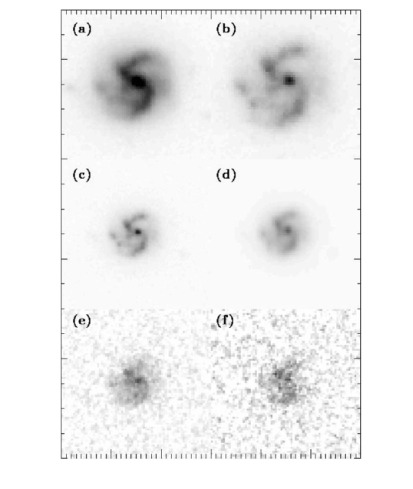
Figure 22: Steps involved in projecting a galaxy to higher redshift. The original image of a galaxy at z=0.47, taken from the HDF (a) is k-corrected to z=1.5 (b), reduced in angular size to match this increased redshift (c), resampled with additional PSF smoothing to compensate for its smaller size (d), and covered with additional noise to match its fainter magnitude (e). Panel (f) matches a 25ks WFPC2 exposure ($\sim 0.7^{m}$ shallower than the HDFs).

B.1 Pixel-by-pixel K-corrections

As discussed above, an important first step in determining the appearance of an object at different redshifts and for different passbands is to calculate its surface brightness distribution at an arbitrary rest-frame wavelength. To this end, we construct a pixel-by-pixel template for an object using the formalism discussed above. For an object observed in the $Y$ band at redshift $z$, the template is equal to the sum of a model term and a correction term

$$I_{i,j}g(SED_{i,j},Y,z)+\Sigma_{X=X_{L}}^{X_{H}}\left(\frac{|\lambda^{Y}-\lambda^{X}\left(\frac{1+z}{1+z_{obs}}\right)|}{\lambda^{X_{H}}\left(\frac{1+z}{1+z_{obs}}\right)-\lambda^{X_{L}}\left(\frac{1+z}{1+z_{obs}}\right)}\right)\left(\frac{1+z}{1+z_{obs}}\right)^{4}\Delta f_{i,j}^{X}$$ (B1)

where $\lambda^{Y}$ is the central wavelength of band $Y$. The band $X$ in the summation above ranges over the passbands whose redshifted central wavelength $\lambda^{X}\left(\frac{1+z}{1+z_{obs}}\right)$ most closely straddles the central wavelength of the observational band $Y$, $\lambda^{Y}$–where $z_{obs}$ is the redshift of the original object on which the templates are based. Hence, for a galaxy originally observed in the $U_{300}$, $B_{450}$, $V_{606}$, $I_{814}$ passbands at $z\sim 3$ and resimulated at $z\sim 4$ in the $V_{606}$ band, $X$ would include both the $B_{450}$ and $V_{606}$ bands, $\lambda^{B_{450}}\left(\frac{1+z}{1+z_{obs}}\right)\sim(450\,\textrm{nm})(5/4)\sim 563\,\textrm{nm}$ and $\lambda^{V_{606}}\left(\frac{1+z}{1+z_{obs}}\right)\sim(606\,\textrm{nm})(5/4)\sim 758\,\textrm{nm}$, straddling the central wavelength of $V_{606}$, $\sim 606\,\textrm{nm}$. Obviously, when $\lambda^{Y}$ is outside the range of the redshifted templates, there will only be one passband $X$ in the above summation.

For the observed redshifts and passbands, Eq. (B1) gives exactly the same images as found in the processed data. Only to the extent that a simulated passband fails to line up with one of the redshifted passbands are the derived templates based upon the best-fit SED templates. Note that this is in contrast to and an improvement over the procedure used in BBSI (where the $\Delta f_{i,j}$ terms were dropped) as it depends less on the details of the SED templates used.

B.2 Geometric Corrections

We then orient the k-corrected galaxy template on our simulated image, scaling the template pixel size according to the canonical angular size-distance relationship,

$$d_{temp}=d_{temp,obs}\frac{D_{A}(z)}{D_{A}(z_{obs})}.$$ (B2)

where $d_{temp}$ is the pixel-size of the projected template, $d_{temp,obs}$ is the pixel-size of the template in the original image, and $D_{A}$ is the angular-size distance relationship. We lay the templates down on the simulated images with a variety of pixel centers and rotation angles.

B.3 Correcting the PSF

After the galaxy template has been laid down on the image it is standard to convolve it with the instrumental PSF, henceforth called PSF-new. Unfortunately, the original galaxy template has already been implicitly convolved with a PSF (henceforth called PSF-implicit-unscaled) by virtue of its being drawn from some set of observations. So, to determine the PSF that still needs to be convolved with the image (hereafter called PSF-corr), one needs to deconvolve PSF-implicit-unscaled scaled according to the angular distance relationship (hereafter, called PSF-implicit-scaled) from PSF-new:

$$\textbf{PSF-corr}*\textbf{PSF-implicit-scaled}=\textbf{PSF-new}$$ (B3)

where $*$ indicates a convolution. Note that by performing the deconvolution on high S/N PSFs rather on the images themselves, we avoid performing any deconvolutions on the observational images themselves and therefore degrading the signal-to-noise.

We employ 50 iterations of the Lucy-Hook algorithm (Lucy 1974) to accomplish this. In each iteration, we compute

$$f(n+1)=f(n)\textbf{PSF-implicit-scaled}*\left[\frac{\textbf{PSF-new}}{f(n)*\textbf{PSF-implicit-scaled}}\right]$$ (B4)

For our initial guess, we take the best-fit $\sigma$’s from fits of our PSFs to Gaussians, and then scale the width of PSF-new by $\sqrt{1-(\sigma_{implicit-scaled}/\sigma_{new})^{2}}$ where $\sigma_{implicit-scaled}$ and $\sigma_{new}$ are the $\sigma$’s of the best-fit Gaussian to PSF-implicit-scaled and PSF-new, respectively. To reduce the number of deconvolutions needed we tabulate results for each pair of PSF-new and PSF-implicit-scaled for 10 different values of $\sigma_{implicit-scaled}/\sigma_{new}$ varying from 0 to 1. We make a simple interpolation between the results. Finally, we convolve PSF-corr with the simulated image.

B.4 Adding Noise

At the end of the process we add noise to each pixel. This is not completely trivial. Since the galaxy templates already contain noise, the simulated images generated from these templates will also contain noise. It is, therefore, necessary when simulating images in B.1 to keep track of how much noise has been added to the individual pixels of the simulated image so we can add the remainder at this step. Note also that before adding this additional noise to the image it is smoothed to reflect the correlation properties of the noise for the images in question, here the HDF drizzled images. The kernel for the drizzled WFPC2 images is given in Williams et al. (1996).

Now, we proceed to describe the task of estimating noise on the galaxy templates derived from Eq. (B1). While one might suppose this task to be relatively straightforward, it is a little more subtle than one might imagine. This subtlety owes itself to the fact that simulated postage stamps are the sum of two terms, a k-corrected model profile $I_{i,j}$ and at least one correction image $\Delta f_{i,j}$, both of which contain noise (see Eq. (B1)). Recall that the model profile $I_{i,j}$ is a fit to the pixel-by-pixel values for a set of images, and so for fits on the outer portion of the postage stamp where the signal is dominated by the noise, both the SED $SED_{i,j}$ and the profile itself $I_{i,j}$ will contain noise, and that once the postage stamp is transposed to another redshift, as per Eq. (B1), this noise will also be present, but its magnitude will depend upon the distribution of best-fit SEDs used to represent that noise and the size of the k-corrections made to each of those best-fit SEDs.

Due to the aforementioned subtleties, perhaps the best way of estimating noise on a galaxy template calculated from Eq. (B1) is in exactly the same way one measures noise off an astronomical image. Unfortunately, not all templates are very large and some are largely covered by an object. A simple workaround was to simulate a set of 15 x 15 noise images to process alongside the postage stamps derived from the raw data. In other words, just as for pixels of an image containing a real object, we determine the best-fit model profiles $I$ and SED templates $SED$ for the noise patch (and correction image(s) $\Delta f$) and then transpose it to the object redshift using Eq. (B1). Of course, at this point, it is quite straightforward to determine the noise properties of the transposed noise patch.

B.5 Analysis of Simulated Images

Having simulated postage stamps using the steps outlined in Appendix B.1-B.4, we use exactly the same computer code to analyse the simulated postage stamps as we use on the original images, e.g., the procedure outlined in Appendix A.1. In contrast to our previous work (BBSI) where we generated large galaxy images and analysed them, we prefer to recover all the properties from small postage stamps on which the object has been added. This speeds up the calculations considerably and allows us to look at the selection effects related to object redshifting independent of those effects related to object overlap.

We do not perform background subtraction on our simulated images because a nonnegligible amount of the template flux itself is typically included in the background determination and thereby biases the magnitudes recovered. Embedding the object in the middle of a much larger image effectively removes this bias, but makes the entire process much more computationally expensive. We therefore exclude the background-subtraction step altogether cognizant of the fact that our simulations effectively ignore a small source of scatter resulting from uncertainties in background subtraction step (estimated to be up to a $\sim 10\%$ effect depending on the object and surface density of its neighbors).

Appendix C Volume Density

The next step is to estimate the volume density of each object in the original sample so that we know how frequently to replicate it in simulated samples. We take the volume density of each object to be equal to

$$n=\frac{1}{V_{avail}}.$$ (C1)

where $V_{avail}$ is the expected effective volume in which the object would fall into the selection sample. Formally, the volume available $V_{avail}$ is taken to be

$$V_{avail}=\Omega\int_{z=0}^{z=\infty}\epsilon(z)\frac{dV}{dzd\Omega}dz$$ (C2)

where $\epsilon(z)$ is the efficiency of detection at each redshift and $\Omega$ is the selection area in steradians. The efficiency $\epsilon(z)$ accounts for the extent to which photometric scatter places a galaxy inside or outside the sample. We calculate $\epsilon(z)$ by Monte-Carlo resimulating and remeasuring the galaxy at different orientation angles using the procedures laid out in Appendix B.1-B.5. We add magnitude scatter to the results using the expected Poissonian and Gaussian noise. Ideally, we would add each galaxy to different parts of a frame with all foreground and background objects present to account for the effects of overlap on object detection and parameter extraction (important for perhaps 2-3% of galaxies) but, due to the high computational cost of recovering object parameters for all sample galaxies over a range of both redshift and galaxy environment, we chose not to do this. In Figure 18, we illustrate Monte-Carlo realizations of the photometry for 3 sample $U$-dropouts as a function of redshift.

Appendix D Challenges

D.1 Uncertainties in Empirical Clone Models

While the procedure of mapping one sample of galaxies to another set of redshifts for comparison with another sample is extremely model independent in principle, uncertainties both in the pixel-by-pixel fluxes and the photometric/spectral redshift necessitate the introduction of small model dependencies into the procedure. Even pixel-by-pixel variations in the amount of intervening hydrogen introduce uncertainties, though studies (e.g. Bershady et al. 1999) have shown that the variation is typically small. For some samples such as a bright ($I<23$) HDF sample with spectroscopic redshifts, these uncertainties are minimal and the results therefore largely model-independent. On the other hand, for other samples where the photometric errors are large and no spectroscopic redshifts are available, some model dependence is almost unavoidable.

From a Bayesian perspective, these model dependencies arise as a dependence on an assumed prior, a problem one has whenever the maximum likelihood distribution isn’t sufficiently narrow. For a bright HDF sample where both the flux and redshift uncertainties are small, the corresponding maximum likelihood distributions are extremely narrow and so there is minimal dependence on the assumed prior. For these cases, there are clear advantages to the present approach where the base model is comprised of a sample of template galaxies with specific redshifts (hereafter called the cloning approach) over other approaches which attempt to model galaxies in a two or three dimensional space, since we have minimal loss of information. On the other hand, in cases where the flux and redshift uncertainties become large, clearly a lower-dimensional model-dependent Bayesian analysis becomes more attractive.

Nevertheless, even in the presence of uncertainties there are ways of making some low-order corrections to the results obtained from the cloning approach if the data are of low S/N. We discuss the corrections in turn. The first difficulty relates to the redshift uncertainty of each galaxy template. Redshift uncertainties result in a certain smoothing of the intrinsic distribution of sizes and luminosities, effectively moving the knee of the luminosity function to higher luminosities. This becomes problematic when there are gradients in the density with which particular objects fill redshift space, as there inevitably are, objects naturally moving from regions of high redshift space density to regions of low redshift space density. One could attempt to correct for this effect by binning the objects in some way and by making some assumption about their intrinsic distribution, i.e., the prior, for this class of object, but in doing so, one would introduce model dependencies. An alternate approach for treating this bias would involve not correcting the bias in the original sample itself, but instead introducing a similar bias in every sample against which one compared the original sample. We have employed neither in our paper because our own simulations have shown that the size of the effect ($<5$%) is much smaller than even the Poissonian variation in our small sample.

While it is of course true that uncertainties in the redshift estimators can bias the predictions of the derived model, a more worrisome issue is the possibility that systematic uncertainties in the redshifts derived would not only bias these same predictions, but bias them severely. Since the reliability of photometric redshifts here depends on the extent to which our spectral templates accurately represent the shape and curvature of the true SEDs, it would be rather easy to make systematic errors across our high redshift samples. Fortunately, a large number of our bright galaxies have spectroscopic redshifts and so the reliability of our photometric redshifts can be checked, at least at brighter magnitudes (see Figure 4).

There are also uncertainties in the pixel fluxes, and these uncertainties will affect both our photometry and other parametric determinations, and such errors will have an effect on whether a galaxy is selected as part of our sample or not. This isn’t a problem if galaxies uniformly populate the parameter space over the selection window since objects will as likely be scattered into a region as out of it. Unfortunately, in the more common case where there are gradients in the way objects fill multi-dimensional parameter space objects will naturally be scattered from the more dense regions to the less dense regions (the Malmquist bias being a well-known example of this). As per uncertainties in redshift, corrections require binning the objects in some manner and making some assumption about their intrinsic distribution or prior.

Not only will the uncertainties in the pixel flux have an effect on whether an object is selected or not, they will have an effect on how an object is resimulated at both lower and higher redshift. For example, if errors in the pixel fluxes result in an object’s seeming redder or bluer than it really is, then the resimulated object will consistently appear redder or bluer than it really is, biasing the determined selection function. Fortunately, for the present situation, this has only a $\sim 3-5\%$ effect on the determined volume density, basically because the bulk of the $U$ dropout objects do not lie very close to the $B-I$ edge of the selection window and therefore the scatter toward intrinsically bluer/redder colours does not appreciably change the volume density of sample objects by much on average.

Despite our emphasis on a model-independent cloning approach, a lower-dimensional parametric approach (discussed above) works well in many cases, as the analysis that Steidel et al. (1999) and Deltorn et al. (2001) make of the $U$ dropouts effectively illustrates. In both studies, conclusions about the $U$-dropout population and its relation to higher redshift populations are made based upon a two-variable parameterization: the absolute magnitude at 1700 $\AA$ and the spectral type. Compared with our work, these analyses have their pros and cons. They are better in the sense that allow a more straightforward treatment of errors in redshift and photometry as detailed in this section and enable one to push fainter by considering probable but not certain detections–i.e., Pozzetti et al. (1998)’s pushing fainter than us in their determination of the $U$ and $B$ luminosity functions through their use of Kaplan-Meier (Lavalley, Isobe, & Feigelson 1992) estimators. They also allow a more proper treatment of objects which are rare enough not to be found in the input sample used for constructing the empirical models. They are worse in the sense that they tend to assume that the joint multivariate distribution of surface brightness, shape, blochiness, or pixel-by-pixel color variation is independent of luminosity or spectral type.

D.2 Object Overlap

Another challenge regards the overlap or deblending of different galaxies. Not only is this a problem when one selects the original sample, but it is also a problem when one resimulates these objects in different environments where they may or may not closely overlap with background/foreground objects. For the former problem, one approach is simply to consider these objects as more complicated isolated galaxies. Of course, if the contaminating object is at a very different redshift from the foreground galaxy, attempts at replicating this object to other redshifts can be a problem, the problem being more significant the more equal the fluxes of the blended objects, the more dissimilar their redshifts. This is just another example of the problems one faces when attempting to derive an empirical model from real objects on real images with all the associated uncertainties in redshifts, pixel fluxes, and possible blending problems. As for the latter problem, it is quite naturally treated by adding the simulated objects to a frame full of foreground and background objects, and treating the blended objects from the simulations just as one does in the real samples. Fortunately, both problems appear to have a very small effect, affecting only $\sim 2$% of the objects (a rough estimate based upon the overlapping objects found in the HDFs). Note that for speed and simplicity, we have measured the properties of sample galaxies in isolation. Not only would a full treatment of overlap require a lot more computational resources, but it would be impossible to do exactly right due to difficulties involved in separating foreground objects from background objects on which they are superimposed.

D.3 Inadequate S/N

Determining the selection window for almost any object requires one to resimulate the galaxy at both lower and higher redshifts. When projected to lower redshifts, the S/N of the template is not generally good enough for an accurate comparison with the real high S/N lower-redshift data. In these cases, we have chosen simply to allow the noise to increase, resulting in a larger scatter in the recovered magnitudes. Obviously, one should pay attention to these issues when interpreting the data or designing the original selection criteria, but they do not introduce any significant systematics here. Another difficulty occurs in trying to simulate objects at very low redshift where the angular extent of objects becomes very large relative to the pixel scale. This significantly increases the simulation time. To speed things up, for cases where the pixel sizes are smaller than the projected size of template pixels, the pixel sizes and zero-points of the simulated images are scaled up to match that of the template pixels.

References

- Adelberger et al. (1998) Adelberger, K. L., Steidel, C. C., Giavalisco, M., Dickinson, M., Pettini, M., & Kellogg, M. 1998, ApJ, 505, 18.
- Benítez et al. (1999) Benítez, N., Broadhurst, T., Bouwens, R., Silk, J., & Rosati, P. 1999, ApJ, 515, L65.
- Benítez (2000) Benítez, N. 2000, ApJ, 536, 571.
- Bershady, Charlton, & Geoffroy (1999) Bershady, M. A., Charlton, J. C., & Geoffroy, J. M. 1999, ApJ, 518, 103.
- Bertin and Arnouts (1996) Bertin, E. and Arnouts, S. 1996, A&AS, 117, 393.
- Bertin and Arnouts (1996) Bertin, E. 2001, ftp:ftp.iap.fr/pub/from_users/bertin/swarp/.
- Bouwens, Broadhurst and Silk (1998) Bouwens, R., Broadhurst, T. and Silk, J. 1998a, ApJ, 506, 557.
- Bouwens, Broadhurst and Silk (1998) Bouwens, R., Broadhurst, T. and Silk, J. 1998b, ApJ, 506, 579.
- Bouwens & Silk (2002) Bouwens, R. & Silk, J. 2002, ApJ, 568, 522
- (10) Bouwens, R.J, et al. 2003, in preparation.
- Broadhurst (1988) Broadhurst, T.J., Ellis, R.S., & Shanks, T. 1988, MNRAS, 235, 827.
- Bruzual A. & Charlot (1993) Bruzual A., G. & Charlot, S. 1993, ApJ, 405, 538.
- Calzetti, Kinney, & Storchi-Bergmann (1994) Calzetti, D., Kinney, A. L., & Storchi-Bergmann, T. 1994, ApJ, 429, 582.
- Cohen et al. (2000) Cohen, J. G., Hogg, D. W., Blandford, R., Cowie, L. L., Hu, E., Songaila, A., Shopbell, P., & Richberg, K. 2000, ApJ, 538, 29.
- Coleman, Wu, & Weedman (1980) Coleman, G. D., Wu, C. -., & Weedman, D. W. 1980, ApJS, 43, 393.
- Connolly et al. (1997) Connolly, A. J., Szalay, A. S., Dickinson, M., Subbarao, M. U., & Brunner, R. J. 1997, ApJ, 486, L11.
- Cowie, Lilly, Gardner, & McLean (1988) Cowie, L. L., Lilly, S. J., Gardner, J., & McLean, I. S. 1988, ApJ, 332, L29.
- Cowie et al. (1999) Cowie, L.L., Songaila, A., & Barger, A.J. 1999, AJ, 118, 603.
- de Jong & Lacey (2000) de Jong, R. S. & Lacey, C. 2000, ApJ, 545, 781
- Deltorn et al. (2001) Deltorn, J.-M. et al. in preparation.
- Dickinson et al. (1999) Dickinson, M., et al. in preparation.
- Fernández-Soto, Lanzetta, & Yahil (1999) Fernández-Soto, A., Lanzetta, K. M., & Yahil, A. 1999, ApJ, 513, 34.
- Giavalisco et al. (1998) Giavalisco, M., Steidel, C. C., Adelberger, K. L., Dickinson, M. E., Pettini, M., & Kellogg, M. 1998, ApJ, 503, 543.
- Glazebrook et al. (1995) Glazebrook, K., Ellis, R., Colless, M., Broadhurst, T., Allington-Smith, J., & Tanvir, N. 1995, MNRAS, 273, 157.
- Guhathakurta, Tyson, & Majewski (1990) Guhathakurta, P., Tyson, J. A., & Majewski, S. R. 1990, ApJ, 357, L9.
- Hogg & Tannis (1993) Hogg, R.V. & Tanis, E. 1993, Macmillian, New York, pg. 428.
- Hibbard & Vacca (1997) Hibbard, J. E. & Vacca, W. D. 1997, AJ, 114, 1741.
- Kinney et al. (1996) Kinney, A. L., Calzetti, D., Bohlin, R. C., McQuade, K., Storchi-Bergmann, T., & Schmitt, H. R. 1996, ApJ, 467, 38.
- Kron (1980) Kron, R. G. 1980, ApJS, 43, 305.
- Lanzetta et al. (2002) Lanzetta, K. M., Yahata, N., Pascarelle, S., Chen, H., & Fernández-Soto, A. 2002, ApJ, 570, 492
- Lavalley, Isobe, & Feigelson (1992) Lavalley, M., Isobe, T., & Feigelson, E. 1992, ASP Conf. Ser. 25: Astronomical Data Analysis Software and Systems I, 1, 245.
- Leitherer & Heckman (1995) Leitherer, C. & Heckman, T. M. 1995, ApJS, 96, 9.
- Lilly et al. (1996) Lilly, S.J., Le Fevre, O., Hammer, F., & Crampton, D. 1996, ApJ, 460, L1.
- Lilly et al. (1998) Lilly, S. et al. 1998, ApJ, 500, 75.
- Lucy (1974) Lucy, L. B. 1974, AJ, 79, 745.
- Madau (1995) Madau, P. 1995, ApJ, 441, 18.
- Madau et al. (1996) Madau, P., Ferguson, H.C., Dickinson, M.E., Giavalisco, M., Steidel, C.C., & Fruchter, A. 1996, MNRAS, 283, 1388.
- Madau et al. (1998) Madau, P., Pozzetti, L. & Dickinson, M. 1998, ApJ, 498, 106.
- Mao, Mo, & White (1998) Mao, S., Mo, H. J., & White, S. D. M. 1998, MNRAS, 297, L71.
- Meier (1976) Meier, D. L. 1976, ApJ, 203, L103.
- Meurer et al. (1997) Meurer, G. R., Heckman, T. M., Lehnert, M. D., Leitherer, C., & Lowenthal, J. 1997, AJ, 114, 54.
- Mo, Mao, & White (1998) Mo, H. J., Mao, S., & White, S. D. M. 1998, MNRAS, 295, 319.
- Papovich & Dickinson (2001) Papovich, C., Dickinson, M., & Ferguson, H.C. 2001, in preparation.
- Pozzetti et al. (1998) Pozzetti, L., Madau, P., Zamorani, G., Ferguson, H.C., & Bruzual, G.A. 1998, MNRAS, 298, 1133.
- Roche et al. (1998) Roche, N., Ratnatunga, K., Griffiths, R. E., Im, M., & Naim, A. 1998, MNRAS, 293, 157.
- (46) Salpeter, E.E. 1955, ApJ, 121, 161.
- Sawicki and Yee (1998) Sawicki, M. and Yee, H. K. C. 1998, AJ, 115, 1329.
- Schmidt et al. (1968) Schmidt, M. 1968, ApJ, 151, 393.
- Steidel & Hamilton (1993) Steidel, C. C. & Hamilton, D. 1993, AJ, 105, 2017.
- Steidel & Hamilton (1992) Steidel, C. C. & Hamilton, D. 1992, AJ, 104, 941.
- Simard et al. (1999) Simard, L. et al. 1999, ApJ, 519, 563.
- Steidel et al. (1999) Steidel, C. C., Adelberger, K. L., Giavalisco, M., Dickinson, M. and Pettini, M. 1999, ApJ, 519, 1.
- Steidel et al. (1998) Steidel, C. C., Adelberger, K. L., Dickinson, M., Giavalisco, M., Pettini, M., & Kellogg, M. 1998, ApJ, 492, 428.
- Szalay, Connolly, & Szokoly (1999) Szalay, A.S., Connolly, A.J., & Szokoly, G.P. 1999, AJ, 117, 68.
- Thompson, Weymann, & Storrie-Lombardi (2001) Thompson, R. I., Weymann, R. J., & Storrie-Lombardi, L. J. 2001, ApJ, 546, 694.
- Treyer et al. (1998) Treyer, M. A., Ellis, R. S., Milliard, B., Donas, J., & Bridges, T. J. 1998, MNRAS, 300, 303.
- Williams, R.E, et al. (1996) Williams, R.E., et al. 1996, AJ, 112, 1335.
- Casertano et al. (2000) Casertano, S., et al. 2000, AJ, 120, 2747.
- Yan et al. (1999) Yan, L., McCarthy, P. J., Freudling, W., Teplitz, H. I., Malumuth, E. M., Weymann, R. J., & Malkan, M. A. 1999, ApJ, 519, L47.