Clusters and Superclusters in the Las Campanas Redshift Survey

We use a 2-dimensional high-resolution density field of galaxies of the Las Campanas Redshift Survey (LCRS) with a smoothing length 0.8 $h^{-1}$ Mpc to extract clusters and groups of galaxies, and a low-resolution field with a smoothing length 10 $h^{-1}$ Mpc to find superclusters of galaxies. We study the properties of these density field (DF) clusters and superclusters, and compare the properties of the DF-clusters and superclusters with those of Abell clusters and superclusters and LCRS groups. We show that among the cluster samples studied the DF-cluster sample best describes the large-scale distribution of matter and the fine structure of superclusters. We calculate the DF-cluster luminosity function and find that clusters in high-density environments are about ten times more luminous than those in low-density environments. We show that the DF-superclusters that contain Abell clusters are richer and more luminous than the DF-superclusters without Abell clusters. The distribution of DF-clusters and superclusters shows the hierarchy of systems in the universe.

1 Introduction

The basic tasks of observational cosmology are to describe the distribution of various objects in the universe and to understand the formation and evolution of these structures. One means for describing the structure is the density field method. In this method the distribution of discrete objects (galaxies and clusters of galaxies) is substituted by the density field calculated by smoothing the discrete distribution. This method has the advantage that it is easy to take into account various selection effects which distort the distribution of individual objects. The density field can be applied to calculate the gravitational field as done in the pioneering study by Davis & Huchra (1982), to investigate topological properties of the universe (Gott et al.  gmd86 (1986)), and to map the universe and to find superclusters and voids (Saunders et al. s91 (1991), Marinoni et al. mar99 (1999), Hoyle et al. h2002 (2002), Basilakos et al. bpr01 (2001)).

In this paper we use the density field of galaxies to find clusters and superclusters of galaxies. This method was introduced by Einasto et al. (2003b , hereafter Paper I) and applied to the Early Data Release of the Sloan Digital Sky Survey. Here we apply the density field method to the Las Campanas Redshift Survey (LCRS). The LCRS is essentially a 2-dimensional survey; however, using the LCRS data we obtain useful information for clusters and superclusters that is not yet available from 3-dimensional surveys of comparable depth. As in Paper I we use the high-resolution density field to find clusters and groups of galaxies as enhancements of the field, and the low-resolution density field to construct a catalogue of superclusters of galaxies. For simplicity, we use the term “DF-clusters” for both groups and clusters found from the high-resolution density field of galaxies; similarly, we use the term “DF-superclusters” for large overdensity regions detected in the low-resolution density field. In identifying the DF-clusters and superclusters we take into account known selection effects. The main selection effect is due to the limited range of apparent magnitudes used in redshift surveys. We assume that galaxy luminosities are distributed according to the Schechter (Schechter76 (1976)) luminosity function, and find the correction for galaxies with luminosities outside the observing window applying the Schechter parameters as found by Hütsi et al. (hytsi02 (2003), hereafter H03) for the LCRS. We shall investigate statistical properties of DF-clusters and superclusters, and study the role of these clusters and superclusters as tracers of the structure of the universe. We compare the distribution of DF-clusters and superclusters with that of the LCRS loose groups (Tucker et al Tucker00 (2000), hereafter TUC), and of Abell clusters and of superclusters traced by Abell clusters (Abell superclusters) (Einasto et al. e2001 (2001), hereafter E01). This study is carried out in the framework of preparation for the analysis of results of the Planck mission to observe the Cosmic Microwave Background radiation.

In Sect. 2 we give an overview of observational data. In Sect. 3 we identify the DF-clusters, discuss selection effects in the LCRS, analyse properties of DF-clusters, and derive the luminosity function of DF-clusters. Similarly, in Sect. 4 we compose a catalogue of DF-superclusters and analyse these systems as tracers of the structure of the universe. Sect. 5 brings our conclusions. In Tables  LABEL:tab:sc1 and LABEL:tab:sc2 we list the DF-superclusters and their identification with conventional superclusters. The three-dimensional distribution of clusters and superclusters, as well as colour versions of the figures with density field maps, are available on the Tartu Observatory website (www.aai.ee/$\sim$maret/cosmoweb.htm).

2 Observational data

2.1 LCRS galaxies and loose groups

The LCRS (Shectman et al. Shec96 (1996) ) is an optically selected galaxy redshift survey that extends to a redshift of 0.2 and covers six $1.5\times 80$ degree slices containing a total of $23,697$ galaxies with redshifts. Three slices are located in the Northern Galactic cap centred at the declinations $\delta=-3^{\circ},\leavevmode\nobreak\ -6^{\circ},\leavevmode\nobreak\ -12^{\circ}$, and three slices are located in the Southern Galactic cap centred at the declinations $\delta=-39^{\circ},\leavevmode\nobreak\ -42^{\circ},\leavevmode\nobreak\ -45^{\circ}$. The thickness of the survey slices at the mean redshift of the survey ($z\approx 0.1$) is approximately $7.5$ $h^{-1}$ Mpc. Throughout this paper, the Hubble constant $h$ is expressed in units of $100$ km s^-1 Mpc^-1.

The spectroscopy of the survey was carried out via a 50 or a 112 fibre multi-object spectrograph; therefore the selection criteria varied from field to field. The nominal apparent magnitude limits for the 50 fibre fields were $m_{1}=16.0\leq R\leq m_{2}=17.3$, and for the 112 fibre fields $m_{1}=15\leq R\leq m_{2}=17.7$. The general properties of the 50 fibre and the 112 fibre groups agree well with group properties found from other surveys. We note that in the case of one slice, $\delta=-6^{\circ}$, all observations were carried out with the 50-fibre spectrograph only. On the basis of the LCRS galaxies TUC extracted a catalogue of loose groups of galaxies; a group had to contain at least 3 galaxies to be included in the catalogue (for more details on the compilation of the group catalogue see TUC). Data on the LCRS slices are given in Table 1: $RA$ – the mean right ascension of the slice, $\Delta RA$ – the width of the slice (both in degrees), $N_{gal}$ – the number of galaxies, $N_{DF}$ – the number of DF-clusters, $N_{LC}$ – the number of loose groups by TUC, $N_{A}$ – the number of Abell clusters, and $N_{scl}$ – the number of DF-superclusters.

Table 1: Data on LCRS galaxies, clusters and superclusters

Slice $$\delta$$

191.4 81.0 4065 1203 289 18 19

189.8 77.9 2323 952 147 13 17

191.4 81.1 4482 1266 276 11 15

12.1 113.8 3922 1285 256 28 18

12.2 112.5 4158 1216 265 19 14

12.3 114.1 3753 1182 263 20 17

2.2 Abell clusters and superclusters

We shall use the catalogue of rich clusters of galaxies by Abell (abell (1958)) and Abell et al. (aco (1989)) (hereafter Abell clusters). All published galaxy redshifts toward galaxy clusters, as well as other data were collected by Andernach & Tago (at98 (1998)). ¿From that compilation we included in our study Abell clusters of all richness classes (but excluded clusters from ACO’s supplementary list of S-clusters) with redshifts up to $z=0.13$. The sample contains 1665 clusters, 1071 of which have measured redshifts for at least two galaxies. This sample was described in detail in E01, where an updated supercluster catalogue of Abell clusters was presented. These E01 superclusters were identified using the friend-of-friends algorithm, first employed in studies of large-scale structure by Turner & Gott (tg76 (1976)) and Zeldovich et al. (zes82 (1982)). All clusters in a supercluster have at least one neighbour at a distance not exceeding the neighbourhood radius of 24 $h^{-1}$ Mpc.

In the present paper we use the E01 catalogue as a reference to identify density field superclusters with conventional ones. In Table 1 and Fig. 2 we have used an updated version (January 2003) of the compilation of redshifts of Abell clusters by Andernach and Tago.

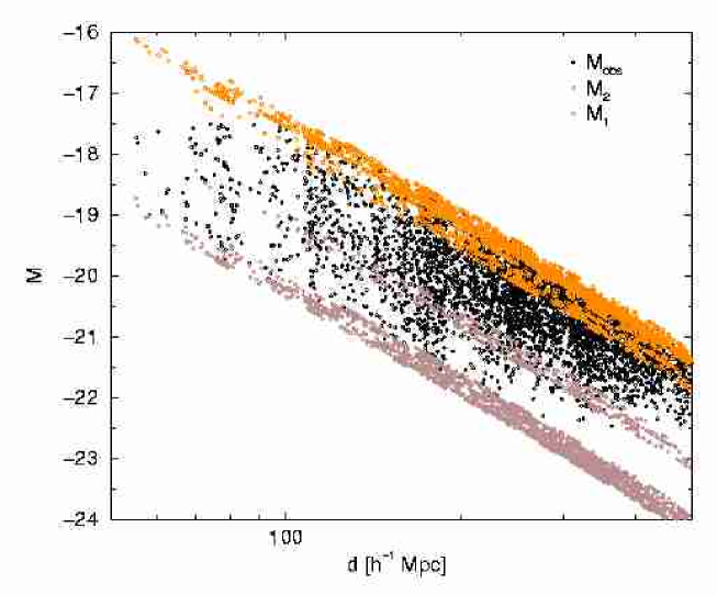
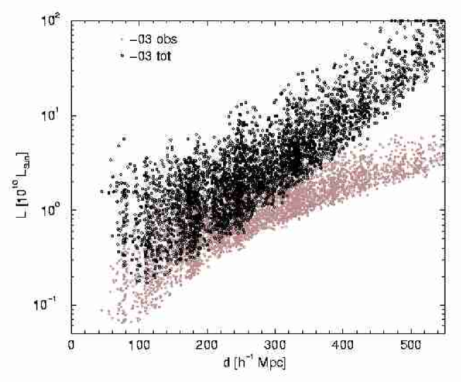
Figure 1: The left panel shows the absolute magnitudes of galaxies, as well as magnitudes of the luminosity window, $M_{1}$ and $M_{2}$, for the $-3^{\circ}$ slice. The right panel gives the luminosities (weights) of galaxies as a function of distance for the same slice. In the left panel black symbols mark the absolute magnitudes of observed galaxies, the upper and lower strips with grey symbols show the absolute magnitude limit $M_{1}$ and $M_{2}$. In the right panel grey symbols show the observed luminosities of galaxies, black symbols are for total luminosities corrected for the unobserved part of the luminosity range.

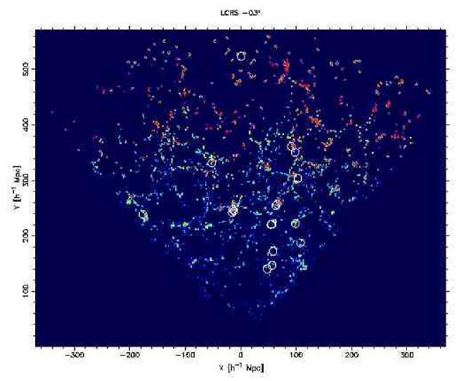
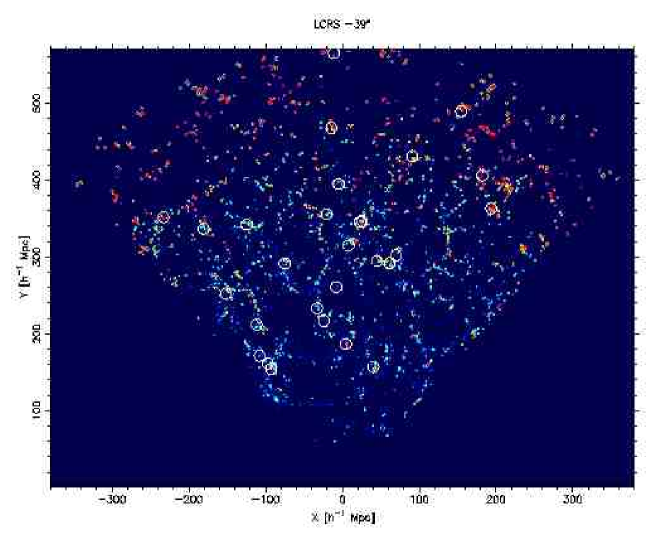
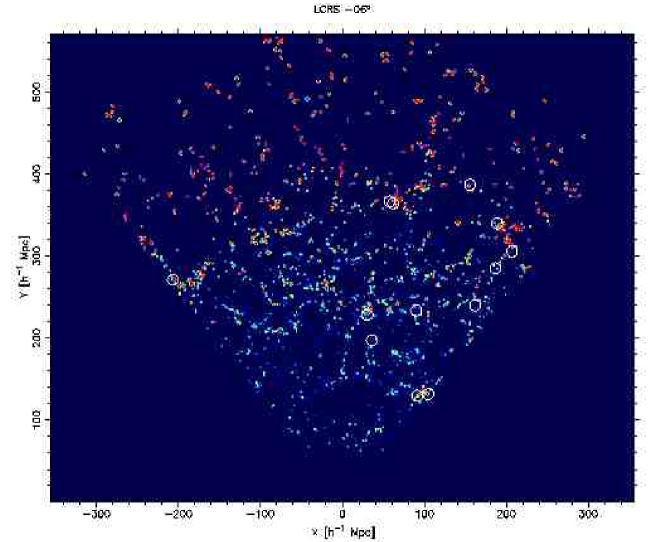
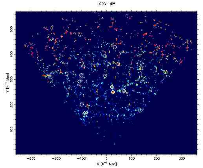
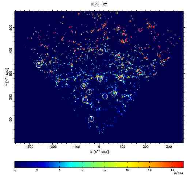
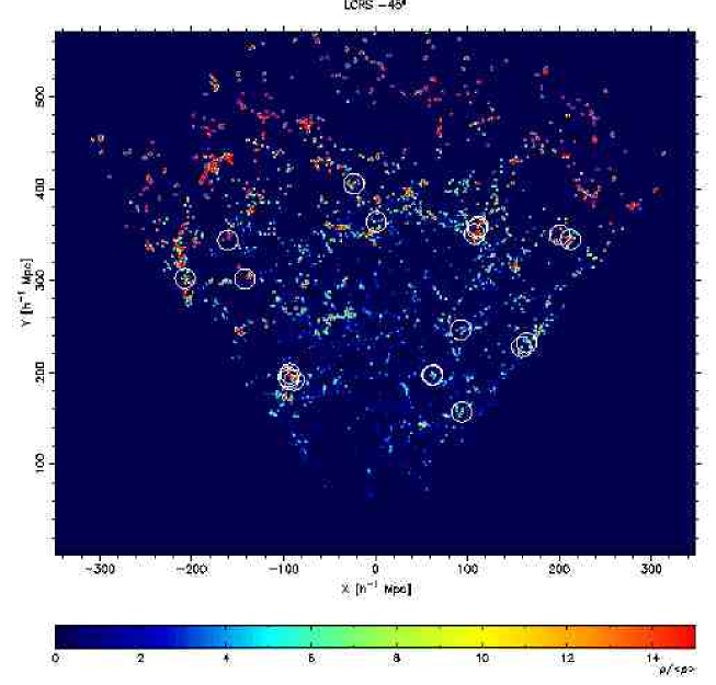
Figure 2: The luminosity density field of the LCRS slices smoothed with a $\sigma=0.8$ $h^{-1}$ Mpc Gaussian filter. Open circles denote positions of Abell clusters located within boundaries of slices. In some cases an Abell cluster consists of several subclusters, in these cases only rich subclusters are marked. The observer is located at the coordinates $(x,y)=(0,0)$.

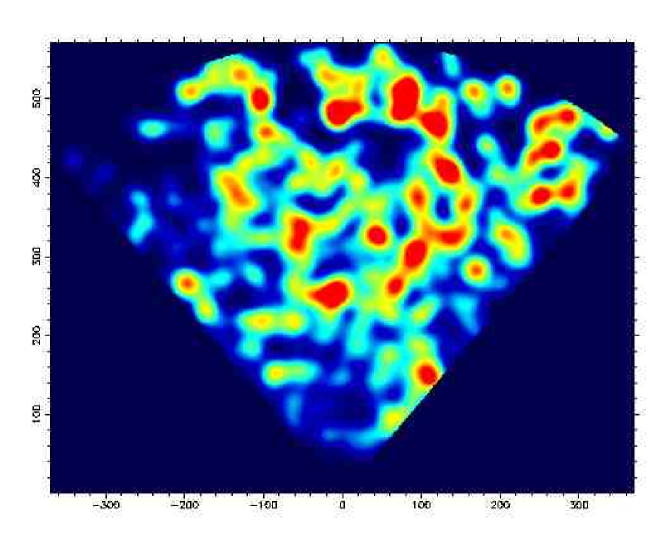
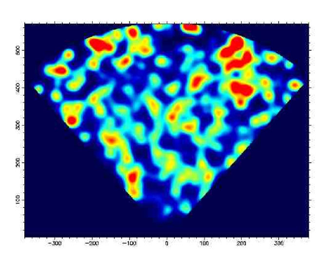
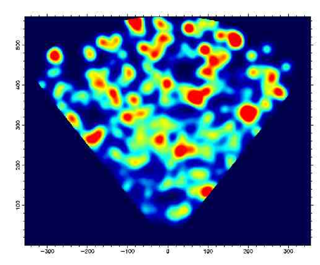
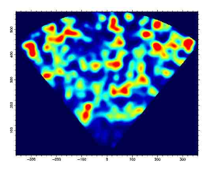
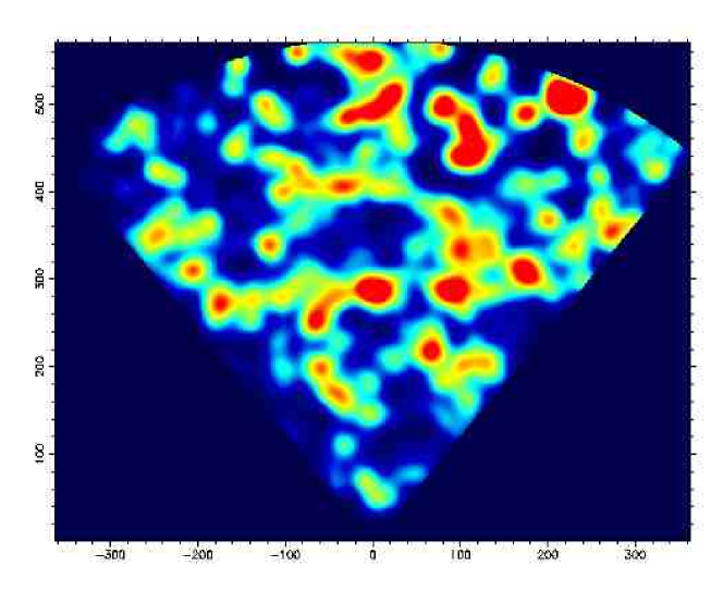
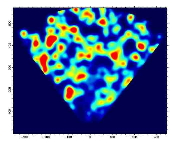
Figure 3: The density field of the LCRS slices smoothed with a $\sigma=10$ $h^{-1}$ Mpc Gaussian filter. Panels are located as in Fig. 2.

3 Density field clusters

3.1 The DF-cluster catalogue

We use the high-resolution density field to find compact overdensity regions. We call these regions density field clusters (DF-clusters). The density field and the DF-clusters were found as follows.

First, we calculated the comoving distance for every LCRS galaxy using a cosmological model with the matter density $\Omega_{\rm m}=0.3$, and the dark energy density (cosmological constant) of $\Omega_{\Lambda}=0.7$ (both in units of the critical cosmological density). In calculating absolute magnitudes we used the K-correction and the correction for absorption in the Milky Way (for details see H03). To calculate the density field we used weights, which take into account the expected luminosity of galaxies outside the visibility window $m_{1}\dots m_{2}$, using a procedure described in Paper I (see also TUC). In doing so we assume that every galaxy is a visible member of a density enhancement. This density enhancement is actually a halo, consisting of one or more bright galaxies in the visibility window, and galaxies fainter or brighter than seen in the visibility window. In calculating the total luminosity of the DF-cluster we assume that luminosities of galaxies are distributed according to the Schechter  (Schechter76 (1976)) luminosity function. The estimated total luminosity per a visible galaxy is

$$L_{tot}=L_{obs}W_{L},$$ (1)

where $L_{obs}=L_{\odot}10^{0.4\times(M_{\odot}-M)}$ is the luminosity of the visible galaxy of absolute magnitude $M$, and

$$W_{L}={\frac{\int_{0}^{\infty}L\phi(L)dL}{\int_{L_{1}}^{L_{2}}L\phi(L)dL}}$$ (2)

is the weight – the ratio of the expected total luminosity to the expected luminosity in the visibility window. In the last equation $L_{i}=L_{\odot}10^{0.4\times(M_{\odot}-M_{i})}$ are the luminosities of the observational window limits corresponding to the absolute magnitudes $M_{i}$, and $M_{\odot}$ is the absolute magnitude of the Sun. In calculating the weights we used the values of the parameters of the Schechter function, $\alpha$ and $M^{\ast}$, as found in H03 (and reproduced in Table 2). Here N50, S50, N112, and S112 denote the 50 and 112 fibre fields in the Northern and Southern hemisphere, and NS112 is the estimate for all the 112 fibre fields. In calculating the weights we integrated instead of 0 to $\infty$ over an absolute magnitude range from $M_{0}=-13.0$ to $M_{lim}=-24.5$ in the R-photometric system.

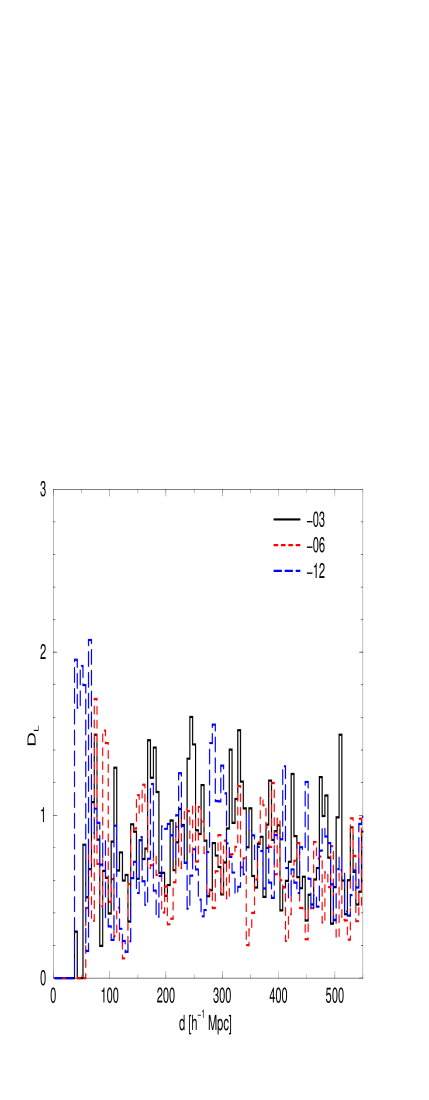
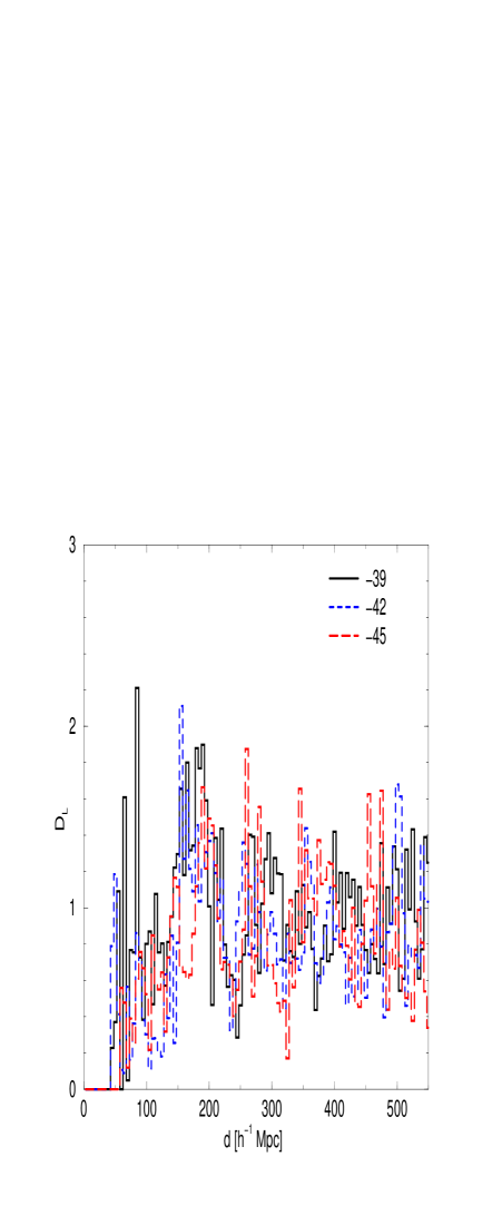
Figure 4: The luminosity density of the LCRS slices as a function of distance. The left panel shows Northern slices, the right panel shows Southern slices.

Table 2: The best fitting $M^{*}$ and $\alpha$ for the LCRS samples

Sample	$M^{*}-5\log h$	$\alpha$
N50	$-\left(20.33\pm 0.12\right)$	$-\left(0.40\pm 0.18\right)$
S50	$-\left(20.64\pm 0.18\right)$	$-\left(0.74\pm 0.21\right)$
N112	$-\left(20.40\pm 0.05\right)$	$-\left(0.76\pm 0.07\right)$
S112	$-\left(20.40\pm 0.05\right)$	$-\left(0.70\pm 0.07\right)$
NS112	$-\left(20.38\pm 0.04\right)$	$-\left(0.70\pm 0.04\right)$
TOTAL	$-\left(20.40\pm 0.03\right)$	$-\left(0.69\pm 0.04\right)$

We plot in Fig. 1 the absolute magnitudes of the window, $M_{1}$ and $M_{2}$, corresponding to the observational window of apparent magnitudes at the distance of the galaxy, and observed absolute magnitudes of galaxies, $M_{obs}$. We also plot in Fig. 1 the estimated total luminosity per visible galaxy (in units of $10^{10}$ solar luminosities) for the $-3^{\circ}$ slice galaxies as a function of distance. This total luminosity was used in calculating the density field.

Fig. 1 shows that the observational window limits $M_{1}$ and $M_{2}$ form several strips in the magnitude–distance diagram. This is due to differences in the apparent magnitude window of the 50 and 112-fibre fields (in particular, in the bright end of the window, where we have several parallel strips of the limit in the left panel of Fig. 1), as well as other observational selection effects discussed by TUC (which increase the width of strips). These differences have been taken into account in the calculation of the luminosity function to find total luminosities for galaxies, and as a result we see no strips in the distribution of total luminosities, plotted in the right panel of Fig. 1.

Next we smoothed the density field with a Gaussian filter of a smoothing length 0.8 $h^{-1}$ Mpc. As described in Paper I, in calculating the density field we used a 2-dimensional grid with a cell size 1 $h^{-1}$ Mpc. This yields a high-resolution map where the individual density enhancements can be easily recognised. This high-resolution density field is presented in Fig. 2. Fig. 3 presents the low-resolution density field found using a 10 $h^{-1}$ Mpc smoothing length. We used this field to find DF-superclusters and to define the global density, characterising the environment of DF-clusters (see Sect. 3.3 below). The high-resolution maps show the density distribution in wedges of increasing thickness as the distance from the observer increases. The low-resolution density maps are converted to sheets of constant thickness by dividing the surface density to the thickness of the sheet at particular distance from the observer.

To identify DF-clusters, every cell of the field was examined to see whether its density exceeds the density of all neighbouring cells. If the density of the cell was higher than that of all its neighbours, then the cell was considered to be the centre of a DF-cluster. The total luminosity of the DF-cluster was determined by summing luminosity densities of cells within a box of size $-2\leq\Delta x\leq 2$, and $-2\leq\Delta y\leq 2$ in cell size units. This range corresponds to the smoothing length 0.8 $h^{-1}$ Mpc which distributes the luminosity of every galaxy between the central and 24 neighbouring cells. The luminosities were calculated in solar luminosity units. At large distances the LCRS sample is rather diluted, and there are only a few galaxies in the nearby region of the LCRS slices. Thus we included into our catalogue of DF-clusters only objects within the distance interval $100\dots 450$ $h^{-1}$ Mpc. The DF-cluster sample has only a few low-luminosity clusters; thus we included in our catalogue only clusters having total luminosities over $L_{0}\geq 0.5\times 10^{10}L_{\odot}$. The number of DF-clusters found in the individual slices is given in Table 1.

According to the general cosmological principle the mean density of luminous matter (smoothed over superclusters and voids) should be the same everywhere. A weak dependence on distance may be due to evolutionary effects: luminosities of non-interacting galaxies decrease as stars age. If we ignore this effect we may expect that the total corrected luminosity density should not depend on the distance from the observer, in contrast to the number of galaxies which is strongly affected by selection (for large distances we do not see absolutely faint galaxies). This difference in observed and total luminosity is clearly seen in Fig. 1: with increasing distance total luminosities exceed observed ones by a factor of ten or more. We can use the mean luminosity density as a test of our weighting procedure. In Fig. 4 we show the mean luminosity density in spherical shells of thickness 5 $h^{-1}$ Mpc for all 6 slices of the LCRS. We see strong fluctuations of the luminosity density, caused by superclusters and voids. The overall mean density is, however, almost independent of the distance from the observer. The mean density is a very sensitive test for the parameters of the luminosity function. It shows that the presently accepted set of parameters of the luminosity function compensates correctly the absence of faint galaxies in our sample.

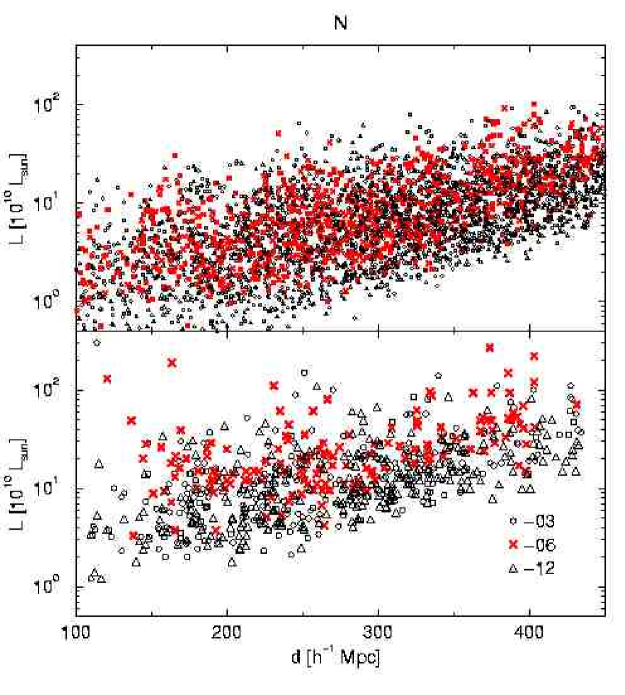
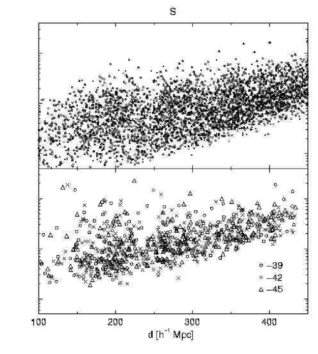
Figure 5: The luminosities of DF-clusters as a function of distance. The upper panels show the distribution for the DF-clusters, the lower panels for the LCRS loose groups; the left panels show Northern slices, the right panels show Southern slices.

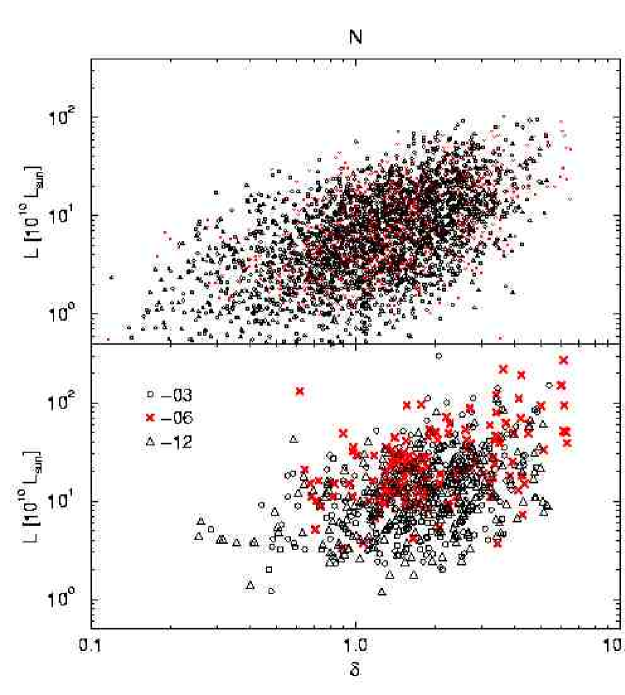
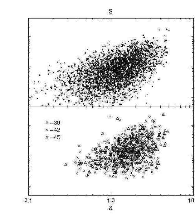
Figure 6: Total luminosities of the DF-clusters (upper panels) and the LCRS loose groups (lower panels) as a function of the global relative density $\delta$. The left panels show Northern slices, the right panels show Southern slices.

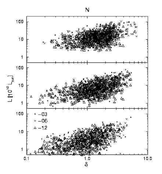
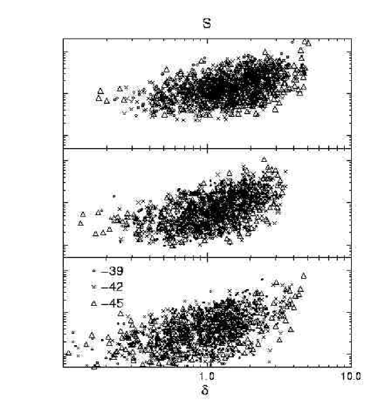
Figure 7: Total luminosities of DF-clusters as a function of the global relative density $\delta$; clusters are divided into 3 distance classes: $100\dots 250$, $250\dots 350$, and $350\dots 450$ $h^{-1}$ Mpc, shown in the lower, middle and upper panels, respectively. The left panels show Northern slices, the right panels show Southern slices.

3.2 Selection effects

The main selection effects in the LCRS (as in the SDSS) are due to the finite width of the apparent magnitude window, $m_{1}\dots m_{2}$, which excludes galaxies outside this window from the redshift survey. This effect reduces the number of galaxies observed for a given structure element (cluster) of the universe. If the cluster contains at least one galaxy within the visibility window of the survey, then the contribution of the remaining galaxies to the expected total luminosity of the cluster can be restored using the weighting scheme discussed above. However, if the cluster has no galaxies in the visibility window, it is lost. For this reason, with increasing distance from the observer, more and more mostly poor clusters disappear from our survey. This effect is clearly seen in Fig. 5, which shows the total luminosities of DF-clusters as a function of the distance from the observer, $d$. For comparison we also show the relationship between the luminosities and distances of the LCRS loose groups of galaxies. We see that low-luminosity clusters are seen only at distances $d\leq 250$ $h^{-1}$ Mpc. This limit is the same for the DF-clusters and the LCRS loose groups, with the difference that there are practically no LCRS loose groups with luminosities less than $2\times 10^{10}\leavevmode\nobreak\ L_{\odot}$, whereas the lower limit of the DF-clusters is $0.5\times 10^{10}\leavevmode\nobreak\ L_{\odot}$, i.e. 4 times lower.

There exists a well-defined lower limit of cluster luminosities at larger distances; this limit is practically linear in the $\log L-d$ plot. Within random fluctuations the lower luminosity limit is identical for most LCRS slices: at 200 and 400 $h^{-1}$ Mpc it is 0.5 and $4.8\times 10^{10}\leavevmode\nobreak\ L_{\odot}$, respectively; only the slice $-6^{\circ}$ has a factor of 2 higher limit. This slice was observed with 50 fibres only, and has a narrower apparent magnitude window. The LCRS loose group sample has at 200 and 400 $h^{-1}$ Mpc a completeness limit of 2 and $16\times 10^{10}\leavevmode\nobreak\ L_{\odot}$, respectively, i.e. a factor of $\sim 3.3$ higher than that for the DF-cluster sample. The absence of low-luminosity clusters at large distances can be taken into account statistically in the calculation of the cluster luminosity function (see below). The location of these missing clusters is not known. Thus with increasing distance there are fewer poor clusters to trace the large-scale structure.

The more luminous DF-clusters and the LCRS loose groups form volume-limited cluster samples; the number of clusters in these samples is, however, considerably smaller than in the full samples. Moreover, the exclusion of poorer clusters would make the investigation of the dependence of cluster richness on environment difficult. The study of the internal structure of superclusters and voids would also be difficult. Thus we have not used volume-limited subsamples of clusters.

In addition to the above selection effect the LCRS has one more problem: due to relatively small number of fibres used in measuring redshifts of galaxies the samples were diluted, i.e. not all galaxies within the observational window $m_{1}\dots m_{2}$ were observed for redshifts. This effect is strong in the $-6^{\circ}$ slice, which was observed only with the 50-fibre spectrograph. For this reason, the number of loose groups detected by TUC in this slice is only about half that of any of the other slices. Similarly, the number of detected DF-clusters is smaller. In calculating the total luminosity of superclusters this additional selection effect is taken into account, so supercluster properties are not affected. The properties of luminous DF-clusters of this slice are similar to the properties of DF-clusters in other slices, and we can conclude that our procedure worked properly.

3.3 Luminosities of DF-clusters in various environment

In Paper I we used the density found with a 10 $h^{-1}$ Mpc smoothing as a parameter to describe the environment in the vicinity of clusters of galaxies. Here we analyse the LCRS DF-clusters and loose groups to investigate the dependence of cluster luminosities on the density of their environment. We calculated the global relative density $\delta$ (in units of the mean density of the low-resolution density field) for all DF-clusters and LCRS loose groups; the results are shown in Fig. 6. As expected from analogy with the SDSS analysis, there is a clear correlation between the luminosity of clusters/groups and the density of their environment. In all LCRS slices the relation between the DF-cluster luminosity and the environmental density is statistically similar. Only in the $-6^{\circ}$ slice are low-luminosity clusters absent due to this slice’s higher luminosity completeness limit.

There exists a well-defined upper limit for the luminosity of the most luminous clusters. DF-clusters in the highest density environments have luminosities up to about $10^{12}\leavevmode\nobreak\ L_{\odot}$. Most luminous loose groups are even brighter – their luminosity in high-density environments goes up to $2.5\times 10^{12}\leavevmode\nobreak\ L_{\odot}$. The most luminous DF-clusters in the lowest density environment have luminosities about $10^{11}\leavevmode\nobreak\ L_{\odot}$, i.e. they are almost one-tenth as luminous. A similar difference was also found for the SDSS clusters. The upper envelope of the luminosity-density relation is statistically identical for all LCRS slices; for the LCRS loose groups this upper envelope is also observed, but over a smaller range of enviromental densities.

Comparing the relationship for the DF-clusters and the LCRS loose groups shows two important differences. First of all, there are very few loose groups in low-density environments, $\delta\leq 0.5$ (we recall that in this plot the environmental density is expressed in the units of the mean density for the whole slice); there are also very few low-luminosity groups. This comparison shows that the LCRS loose groups are much less suitable for studying the structure of the universe in low-density regions. The other difference is observed in the regions of high environmental density. Here the dispersion of luminosities of loose groups is larger than that of DF-clusters. In other words, in high-density environments there are both high-luminosity as well as low-luminosity loose groups, whereas most DF-clusters in high-density environments tend to be quite luminous. The reason for this disagreement between the DF-clusters and the LCRS loose groups is not yet understood.

One may ask whether the cluster luminosity-density dependence could be explained by selection effects, i.e. by the relationship between cluster luminosities and distances shown in Fig. 5. To clarify this problem we divided the DF-clusters into three distance classes and derived the luminosity-density relationship separately for each distance class. The results are shown in Fig. 7. Here the dependence of the cluster luminosity on the density of the environment is seen quite clearly, so this effect must be an intrinsic property of clusters of galaxies. Luminous clusters are predominantly located in high-density regions, poor clusters in low-density regions.

The luminosity-density relation can also be inverted, telling us that we obtain a higher environmental (luminosity) density in a given region if the DF-clusters there are more luminous. As the environmental luminosity density comes mainly from summing up the luminosities of individual DF-clusters, this conclusion is trivial. Fitting a power-law density-luminosity relationship to the data in Fig. 6, we obtain a simple linear law, $\delta\sim L$; this means that this simplest model may indeed be correct. Of course, this fact does not exclude other, more complicated models of the luminosity-density dependence.

The most luminous DF-clusters in high-density environments exceed in luminosity the most-luminous DF-clusters in low-density environments by a factor of 10, as also found for the SDSS clusters in Paper I. The upper envelope of the cluster luminosity-density distribution is very well defined, as seen in Figs. 6 and 7. The lower envelope is not so sharp as the upper one, and it is defined best for nearby clusters (see the lower panels of Fig. 7).

This tendency is seen also in Fig. 2. In the colour-coded version of this figure (http://www.aai.ee/$\sim$maret/cosmoweb), we see that clusters in low-density regions appear blue, which indicates medium and small densities, whereas rich clusters, which appear red in this figure, dominate the central high-density regions of superclusters. This difference is very clear in nearby regions up to a distance $\sim 300$ $h^{-1}$ Mpc. At large distances from the observer poor clusters cannot be observed. Thus, at these distances, all clusters in our appear red in our colour-coded map.

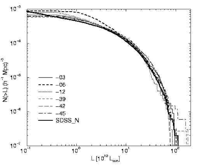
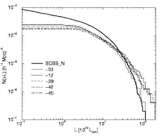
Figure 8: The left panel shows the distribution of luminosities of DF-clusters (the cluster luminosity function) in the LCRS slices. The right panel shows the LCRS loose group luminosity functions. For comparison we show the cluster luminosity function for the SDSS Northern slice (Paper I).

3.4 The luminosity function of DF-clusters

As in Paper I we calculated the integrated luminosity function of DF-clusters, i.e. the number of DF-clusters per unit volume exceeding the luminosity $L$. As we have seen in previous sections, only the brightest DF-clusters can be observed over the whole depth of our samples. We used two methods to calculate the luminosity function: the nonparametric histogram method, and the maximum likelihood method. In the first method we corrected for the incompleteness of less luminous clusters by multiplying the number of observed clusters at each luminosity step by the ratio $(d_{lim}/d_{L})^{3}$, where $d_{lim}=450$ $h^{-1}$ Mpc is the limiting distance of the total sample, and $d_{L}$ is the maximum distance where DF-clusters of luminosity $L$ can be observed. The limiting distance for every $L$ value can be extracted from Fig. 5; we used here a linear relation between $d_{L}$ and $\log L$.

The luminosity function for all 6 slices is shown in Fig. 8. It spans almost 3 orders of magnitude in luminosity and 4 orders of magnitude in spatial density. The difference between individual slices is very small. Only the slice $-3^{\circ}$ has a slightly higher density at low luminosities than the other slices. Here the data have probably been over-corrected for non-observed poor clusters. For comparison we plot the cluster luminosity function for the SDSS Northern slice (Paper I). As we see there is excellent agreement between the LCRS and the SDSS Northern slice data.

We also calculated the luminosity function of the LCRS loose groups of galaxies; this function is shown in the right panel of Fig. 8. Here we used group luminosities as given by TUC. The comparison with the DF-cluster luminosity function shows that the luminosity of the most luminous groups is higher than in the case of the DF-clusters (this is seen also in Figs. 5 and 6). Another difference is in the range of poor clusters. The number of the LCRS loose groups of a given luminosity is much lower than the number of the DF-clusters for the same luminosity. At $L=2\times 10^{10}\leavevmode\nobreak\ L_{\odot}$ the mean integrated densities of the LCRS DF-clusters and loose groups are $4.0\times 10^{-4}$  ($h^{-1}$ Mpc)^-3 and $1.9\times 10^{-4}$ ($h^{-1}$ Mpc)^-3, respectively. For comparison we note that the densities of the SDSS DF-clusters at the same luminosity level are $3.5\times 10^{-4}$ ($h^{-1}$ Mpc)^-3 and $2.9\times 10^{-4}$ ($h^{-1}$ Mpc)^-3 for the Northern and Southern slice, respectively. The lower spatial density of the LCRS loose groups may be explained by a selection effect inherent in the definition of a loose group: here at least 3 galaxies must be present in the group within the observational window, whereas in the case of DF-clusters only one galaxy is needed. Heinämäki et al. (hei2003 (2003)) has calculated the mass function of LCRS loose groups. This function also shows a lower spatial density of loose groups in the poor cluster range.

As a second method, we describe the observed luminosity function by the gamma-distribution, suggested by Schechter (Schechter76 (1976)):

$$\Phi(L)dL=Ax^{\alpha}\exp(-x)dx,$$ (3)

where $x=L/L^{\star}$ is the luminosity in dimensionless units, $L^{\star}$ is the characteristic luminosity of clusters, $A$ is the normalisation amplitude, and $\alpha$ is the shape parameter. We find the estimates of the parameters $L^{\star}$ and $\alpha$ by the maximum likelihood method (Yahil et al.yahil91 (1996)), minimising the log-likelihood function

$${\cal L}=-\sum_{i}^{N}\log(p_{i}),$$

where $N$ is the number of DF-clusters and $p_{i}$ is the probability density for observing the cluster $i$:

$$p_{i}=\frac{\Phi(L_{i})}{\int_{Lm(d_{i})}^{Lu}\Phi(L)dL}.$$

Here $Lu$ is the upper limit of cluster luminosities ($200\times 10^{10}L_{\odot}$ in our case), and $Lm(d_{i})$ is the lower luminosity limit for observed clusters for the cluster distance $d_{i}$. As discussed previously, this limit is rather well defined (see Fig. 5), although it is not easy to predict theoretically. We defined this limit as the lower convex hull of the $d$ vs $L$ diagram.

The shape parameters for the separate slices and for the full DF-cluster sample are given in Table 3. The errors are estimated by approximating the error distributions by the appropriate $\chi^{2}$ distributions, as in Lin et al. (lin96 (1996)). The rms errors given in the table are those for the 1-D marginal distributions.

Table 3: Shape parameters of the Schechter luminosity function for the DF-clusters of the LCRS slices. The slices are marked by their central declination $\delta$ (the first column in the table). The last row gives the luminosity function parameters for the full LCRS DF-cluster sample.

$\delta(^{\circ})$	$L^{\star}(10^{10}L_{\odot})$	$\alpha$
$-$03	15.8$\pm$1.2	-0.55$\pm$0.07
$-$06	15.2$\pm$1.3	-0.52$\pm$0.07
$-$12	14.4$\pm$1.1	-0.70$\pm$0.06
$-$39	16.1$\pm$1.1	-0.51$\pm$0.06
$-$42	13.4$\pm$0.9	-0.42$\pm$0.06
$-$45	19.1$\pm$1.5	-0.71$\pm$0.06
total	14.4$\pm$0.2	-0.43$\pm$0.01

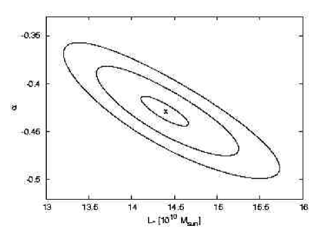
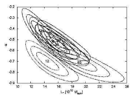
Figure 9: The 1$\sigma$, 2$\sigma$, and 3$\sigma$ confidence regions for the Schechter function parameters $L^{\star}$ and $\alpha$. The upper panel shows the confidence regions for the total sample and the lower panel – the regions for individual samples. Note that the scales in the panels are different. The confidence regions in the lower panel are marked by the slice number in their centres.

The 2-D 1$\sigma$, 2$\sigma$ and 3$\sigma$ (68.3%, 95.4%, and 99.7%) confidence regions are shown in Fig. 9. As we approximated the error distribution rather freely, choosing the $\chi^{2}$ distribution for this purpose, these confidence levels are approximate. This is especially true for the confidence levels for the outer regions, since the Schechter distribution has rather strong wings. The confidence regions for the total sample, shown in the upper panel of Fig. 9, are nice and narrow, but this does not tell the whole story. The lower panel of Fig. 9 shows that the confidence regions of the parameter estimates for individual slices differ considerably. The slice group $-03^{\circ}$, $-06^{\circ}$, and $-39^{\circ}$ has similar luminosity functions, the two slices $-42^{\circ}$ and $-45^{\circ}$ are close to that group, but the luminosity function for the slice $-12^{\circ}$ differs considerably from the rest. Estimating the rms errors of the parameters of the luminosity function for the full sample from the scatter of the results for the individual slices, we find $L^{*}=(14\pm 3)\times 10^{10}\leavevmode\nobreak\ L_{\odot}$, $\alpha=-0.44\pm 0.15$.

To compare the LCRS DF-cluster luminosity function with that for the SDSS slices, we also determined the Schechter parameters for these data. We get for the SDSS Northern slice the characteristic luminosity $L^{*}=19\times 10^{10}\leavevmode\nobreak\ L_{\odot}$, the shape parameter $\alpha=-0.9$, and the amplitude $A=4.5\times 10^{-4}$  ($h^{-1}$ Mpc)^-3; for the Southern slice, $L^{*}=9\times 10^{10}\leavevmode\nobreak\ L_{\odot}$, $\alpha=-0.5$, and the amplitude $A=10\times 10^{-4}$  ($h^{-1}$ Mpc)^-3.

We discussed above that at large distances poor DF-clusters are not visible. This is seen in the Fig. 5 luminosity vs. distance plot, as well as in Fig. 2, where all distant clusters have a reddish colour. The mean luminous density is almost independent of distance, as seen from Fig. 4. The mean constant level of global density in the absence of poor clusters is possible only if the luminous density due to invisible clusters (all galaxies lying outside the visibility window) is added to luminous visible clusters. As discussed in Paper I, this effect makes distant clusters too luminous. Fig. 5 shows that the luminosity of the brightest DF-clusters indeed increases with distance. To get correct luminosities for the DF-clusters we used in Paper I a second set of parameters of the Schechter function to calculate weights of visible galaxies. Here we shall use a different procedure to get correct luminosities for the DF-clusters.

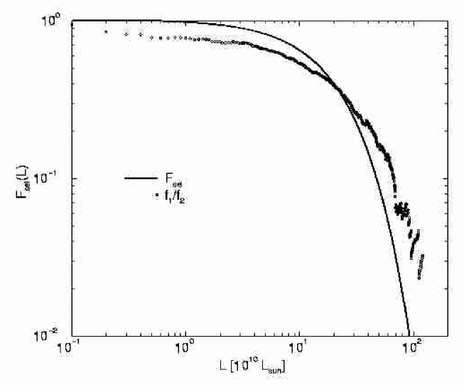
Figure 10: The cluster luminosity selection function, determined by two methods. The solid line shows the selection function found in this paper using Eq. (4). Dots give the selection function as found in Paper I using two sets of parameters of the Schechter function.

The fraction of the expected sum of luminosities of visible clusters to the sum of luminosities of all clusters above a certain threshold at a given distance from the observer can be found by

$$F_{sel}(L)={\int_{L}^{\infty}\Phi(L)LdL\over\int_{L_{0}}^{\infty}\Phi(L)LdL},$$ (4)

where $L_{0}=0.5\times 10^{10}L_{\odot}$ is the lower limit of luminosities of our cluster sample. Using the set of Schechter parameters for the SDSS Northern sample (which approximates well the mean of the LCRS samples) we calculated the selection function $F_{sel}(L)$; the results are shown in Fig. 10. For comparison we show also the selection function as found in Paper I using two sets of parameters of the Schechter function, by dividing the luminosity functions for both parameter sets at a given luminosity $L$. The overall agreement of the selection functions calculated by different methods is satisfactory. The method used in this paper is more physically motivated. The correction factor to calculate the unbiased values of cluster luminosities is $1/F_{sel}(L)$; here the luminosity $L$ is distance dependent and should be calculated from the lower threshold of the luminosities of the DF-clusters at a given distance, as shown in Fig. 5. At the limiting distance $d_{lim}=450$ $h^{-1}$ Mpc the threshold luminosity is $L=8\times 10^{10}L_{\odot}$, and here $F_{sel}=0.72$ (i.e. the luminosities of DF-clusters at this distance must be decreased by a factor of 1.4). We see that this selection effect is rather modest.

Presently we have no data for the masses of DF-clusters. Thus we are unable to convert the luminosity function to the cluster mass function. Even so, the luminosity function is interesting in and of itself. It is less distorted by random errors (which influence masses of individual clusters) and it can be easily determined for all clusters independently of the number of galaxies observed in the cluster. Comparison with the SDSS data shows excellent agreement.

4 Density field superclusters

4.1 The DF-supercluster catalogue

We define superclusters of galaxies as the largest non-percolating density enhancements in the universe (Einasto et al. e1997 (1997)). Superclusters can be identified using either galaxy or cluster data. Here we use the low-resolution density field to find large overdensity regions which we call density field superclusters (DF-superclusters). This field was calculated using the galaxy data and corrected to account for galaxies outside the visibility window. The density field was Gaussian-smoothed, using the smoothing length $\sigma_{sm}=10$ $h^{-1}$ Mpc, which eliminates small-scale irregularities and the ’finger-of-god’ effect. To reduce the conical volume of slices (wedges) to an identical thickness we divided densities by the thickness of the slice at the particular distance. In this way the surface density of the field is in the mean constant. This reduced density field for all 6 LCRS slices is shown in Fig. 3.

Figure 11: Properties of the LCRS density field superclusters as a function of the threshold density, $\delta$, that separates superclusters (high-density regions) and voids (low-density regions). The upper panel shows the number of superclusters, $N$, the middle panel shows the area of the largest supercluster (in units of the total area covered by superclusters), and the lower panel shows the size (either in the $x$ or $y$ direction, whatever is larger) of the largest supercluster.

Table 4: The list of Northern superclusters

$No$	$\delta_{max}$	$L_{tot}$	$L_{D}$	$D$	$\Delta$	RA	$d$	$x$	$y$	$f$	$N_{DF}$	$N_{LC}$	$N_{A}$	Ident	Type
				Mpc	Mpc	deg	Mpc	Mpc	Mpc
(1)	(2)	(3)	(4)	(5)	(6)	(7)	(8)	(9)	(10)	(11)	(12)	(13)	(14)	(15)	(16)
-03.01	3.7	1565	2595	31	39	156	184	106	151	0.0290	23	22	0	88	D
-03.02	2.1	161	379	14	18	156	114	65	94	0.0057	4	3	0		D
-03.03	2.6	666	1418	26	37	158	382	211	319	0.0196	9	0	0		F
-03.04	2.8	485	919	20	23	160	328	169	282	0.0119	13	0	0		M
-03.05	2.7	26798	20113	89	212	172	348	107	331	0.2306	124	29	4	100	M
-03.05a	2.9	582	1008	20	28	168	397	155	365	0.0179	10	0	0		C
-03.05b	2.7	8822	9526	59	106	171	315	105	297	0.1516	64	20	3	100	D
-03.05c	4.9	1498	3695	34	43	173	430	130	410	0.0511	12	0	0		M
-03.05d	3.0	625	1537	24	37	177	383	95	372	0.0267	9	1	1	265	M
-03.06	3.9	957	2480	30	36	183	329	42	326	0.0269	17	4	0		M
-03.07	2.1	185	307	12	15	189	394	18	394	0.0046	4	0	0		F
-03.08	2.4	527	1079	23	33	193	404	-14	404	0.0155	5	0	0		D
-03.09	2.2	268	523	16	22	196	420	-41	418	0.0077	5	0	0		F
-03.10	5.4	3266	5871	44	75	197	249	-26	248	0.0572	26	7	3	126	M
-03.11	2.0	114	214	10	15	199	397	-55	393	0.0033	2	0	0		F
-03.12	3.4	3994	5073	45	68	199	328	-41	326	0.0606	41	3	1		M
-03.13	2.0	98	231	11	14	205	438	-103	426	0.0036	2	0	0		C
-03.14	2.1	121	351	13	17	207	226	-64	217	0.0053	4	1	0		F
-03.15	2.0	173	303	12	16	208	432	-122	415	0.0046	5	0	0		F
-03.16	2.7	1979	3206	37	51	211	404	-135	381	0.0417	28	3	0		M
-03.17	2.2	210	575	17	25	216	240	-103	217	0.0084	6	2	0		C
-03.18	2.1	157	321	12	16	220	173	-84	151	0.0048	5	5	0		F
-03.19	2.8	422	1000	21	24	228	330	-197	264	0.0129	9	0	0	155	M
-06.01	2.2	197	398	18	17	154	427	242	352	0.0064	2	0	0		D
-06.02	4.3	1697	2745	40	53	156	160	88	134	0.0318	18	8	1	88	M
-06.03	6.5	3911	6787	54	51	157	384	200	328	0.0596	23	2	2		M
-06.04	1.9	88	252	14	19	166	192	76	176	0.0044	5	0	0		D
-06.05	6.5	5728	7650	62	76	179	379	73	372	0.0774	32	3	2	268	M
-06.06	4.6	3632	5197	55	63	179	244	42	240	0.0616	34	10	1		M
-06.07	3.6	993	2027	36	35	190	401	-3	401	0.0257	6	0	0		F
-06.08	2.0	95	363	17	18	191	304	-9	304	0.0062	3	0	0		D
-06.09	3.4	1412	2554	41	39	194	264	-23	263	0.0336	23	3	0		D
-06.10	2.6	624	984	27	29	202	439	-97	429	0.0144	7	0	0		F
-06.11	2.9	418	1114	28	25	202	372	-86	362	0.0154	6	0	0		D
-06.12	3.4	2446	3402	48	65	204	332	-85	321	0.0461	23	1	0		D
-06.13	2.0	139	329	16	18	204	278	-69	269	0.0056	5	0	0		D
-06.14	2.2	283	617	22	27	210	222	-79	208	0.0101	8	1	0		F
-06.15	3.4	3797	5494	61	85	211	419	-157	389	0.0753	18	1	0		D
-06.16	4.0	2198	3924	47	50	224	327	-185	270	0.0449	20	3	1		M
-06.17	3.0	622	1288	29	28	226	395	-239	314	0.0177	7	0	0		F
-12.01	2.9	711	2576	43	49	153	455	274	363	0.0352	8	0	0		D
-12.02	2.2	300	664	23	23	156	407	228	338	0.0100	7	1	0		D
-12.03	4.0	2077	3625	46	45	161	352	173	307	0.0400	26	4	0		D
-12.04	2.5	428	658	22	20	162	417	199	367	0.0093	7	0	0		C
-12.05	2.5	1412	2467	43	63	162	224	107	197	0.0354	15	11	0		M
-12.06	3.1	15786	12738	91	123	173	341	104	325	0.1556	99	21	3	105	M
-12.07	3.6	1312	2354	39	39	174	228	65	219	0.0282	20	10	0		M
-12.08	3.5	9329	9187	73	107	197	271	-26	270	0.0994	64	26	2	118	M
-12.09	2.4	6553	6219	68	142	198	418	-50	415	0.0870	42	0	0		M
-12.10	2.7	2433	2820	45	57	207	186	-49	180	0.0382	20	19	1	141	M
-12.11	2.8	377	847	24	23	211	358	-118	338	0.0114	7	0	0		C
-12.12	2.1	383	602	22	28	211	299	-101	281	0.0093	11	0	0		F
-12.13	2.1	1613	2627	43	61	222	314	-158	271	0.0353	21	4	1	156	M
-12.14	2.8	517	1011	27	25	226	371	-207	308	0.0135	7	0	0		D
-12.15	2.5	776	1418	33	33	227	427	-246	349	0.0202	17	0	1		D

Table 5: The list of Southern superclusters

$No$	$\delta_{max}$	$L_{tot}$	$L_{D}$	$D$	$\Delta$	RA	$d$	$x$	$y$	$f$	$N_{DF}$	$N_{LC}$	$N_{A}$	Ident	Type
				Mpc	Mpc	deg	Mpc	Mpc	Mpc
(1)	(2)	(3)	(4)	(5)	(6)	(7)	(8)	(9)	(10)	(11)	(12)	(13)	(14)	(15)	(16)
-39.01	2.1	153	380	17	16	316	308	199	235	0.0062	3	1	0		F
-39.02	2.1	202	303	15	14	316	263	170	200	0.0049	3	1	0		C
-39.03	2.1	363	328	16	15	319	410	260	317	0.0053	6	0	0		C
-39.04	2.4	500	754	24	25	325	195	109	162	0.0114	8	3	0		F
-39.05	3.7	9818	9652	74	84	335	430	193	384	0.1086	40	0	1		M
-39.06	2.0	214	253	14	14	337	215	94	193	0.0042	4	1	0		F
-39.07	2.3	534	673	23	23	341	358	138	331	0.0104	9	0	0		M
-39.08	3.2	2955	3347	47	48	355	423	84	415	0.0435	22	0	1		D
-39.09	2.6	986	1498	33	35	356	300	58	295	0.0217	12	2	3	9	M
-39.10	2.5	1740	2609	43	53	6	332	20	332	0.0373	16	4	2	5	M
-39.11	2.1	607	766	25	37	7	199	8	199	0.0126	7	4	1		M
-39.12	2.1	270	328	16	15	8	396	14	396	0.0054	4	0	0		D
-39.13	2.3	920	1154	30	37	19	352	-37	350	0.0179	11	0	0		M
-39.14	2.4	618	754	24	24	48	417	-195	369	0.0116	6	0	0		M
-39.15	2.1	296	403	18	19	49	384	-179	340	0.0065	6	1	1		F
-39.16	2.9	5162	3960	54	79	51	276	-136	240	0.0578	37	12	1	48	M
-39.17	3.6	4702	4455	55	76	53	172	-92	145	0.0589	33	28	3	48	M
-39.18	3.9	4893	4296	54	59	64	412	-253	326	0.0584	32	0	1		D
-42.01	2.0	131	241	14	13	321	310	179	254	0.0042	3	0	0		M
-42.02	2.4	415	613	22	21	321	401	233	327	0.0098	8	0	1		M
-42.03	2.4	688	1022	28	34	321	214	122	176	0.0163	11	10	1	182	F
-42.04	3.0	1975	2715	43	46	336	332	136	303	0.0388	21	3	0		M
-42.05	2.4	538	993	27	33	341	369	133	345	0.0156	7	0	1		F
-42.06	3.6	8142	6669	66	93	353	269	60	263	0.0886	48	14	3	222	M
-42.07	3.4	4840	4775	57	68	4	376	29	375	0.0657	31	3	1		M
-42.08	2.7	1039	1437	32	32	20	356	-45	354	0.0213	17	0	0		M
-42.09	1.8	139	281	15	25	22	267	-41	264	0.0050	3	1	0		F
-42.10	2.0	200	328	16	20	30	365	-91	353	0.0056	3	1	1		F
-42.11	3.5	5454	5404	57	75	47	188	-81	170	0.0680	36	21	1	48	M
-42.12	2.0	180	369	17	18	50	427	-197	379	0.0064	3	0	0		F
-42.13	2.4	648	848	25	25	52	382	-188	332	0.0132	8	0	0		D
-42.14	3.4	1767	2362	39	43	65	394	-236	316	0.0308	19	0	1		M
-45.01	2.7	1193	1391	32	34	317	291	170	236	0.0203	15	2	2	183	F
-45.02	3.2	822	1499	31	30	325	401	204	345	0.0199	10	0	2		D
-45.03	2.5	789	1044	28	27	327	181	89	158	0.0159	11	5	1	182	D
-45.04	2.1	470	763	25	32	340	262	92	245	0.0125	9	1	1	197	M
-45.05	5.0	6838	6926	65	80	342	366	121	345	0.0846	47	2	3	206	M
-45.06	2.2	321	560	21	22	343	149	48	141	0.0089	4	4	0		C
-45.07	3.0	2220	2595	43	45	1	387	42	385	0.0366	24	3	0		D
-45.08	2.9	5184	4863	59	71	16	365	-23	364	0.0687	39	4	1		M
-45.09	2.8	1319	1577	33	35	20	434	-53	431	0.0226	13	0	0		D
-45.10	3.4	2710	3635	48	52	24	261	-44	258	0.0471	23	14	0		M
-45.11	2.1	256	628	22	24	36	283	-87	269	0.0104	5	1	0		F
-45.12	3.1	1310	1867	35	37	38	408	-132	387	0.0249	15	0	0		D
-45.13	2.7	556	885	25	24	46	384	-159	350	0.0129	6	0	1		F
-45.14	2.5	544	709	23	22	47	337	-141	306	0.0107	3	0	1		C
-45.15	4.7	6505	5971	57	61	48	205	-91	184	0.0643	37	20	4	48	M
-45.16	2.7	505	766	23	21	58	284	-147	243	0.0110	3	0	0		C
-45.17	4.8	11496	9387	71	94	64	388	-220	319	0.1019	53	6	1		M

In the density field approach superclusters can be identified as connected, high-density regions. The remaining low-density regions can be considered voids. To divide the density field into superclusters and voids we need to fix the threshold density, $\delta$, which divides the high- and low-density regions. This threshold density plays the same role as the neighbourhood radius used in the friends-of-friends (FoF) method to find clusters in galaxy samples or superclusters in cluster samples (for a more detailed discussion see Paper I). To make a proper choice of the threshold density we plot in Fig. 11 the number of superclusters, $N$, the area of the largest supercluster $P$ (in units of the total area covered by superclusters), and the maximum size of the largest supercluster (either in the $x$ or $y$ direction), as a function of the threshold density $\delta$ (we use relative densities as above). The data are given for all 6 slices. We see that the number of superclusters has a maximum at $\delta=1.3\dots 1.8$. The diameters of superclusters decrease with increasing threshold density. At a low threshold density the largest superclusters have several concentration centres (local density peaks), their diameters exceed 100 $h^{-1}$ Mpc, and their area forms a large fraction of the total area of superclusters. We have accepted the threshold density $\delta=1.8$; the same value was also used in Paper I for the density field of the Sloan Digital Sky Survey. This threshold density defines compact and rather rich superclusters. If we want to get a sample of poor or medium rich superclusters then we would need to use a lower threshold density, with the price of getting supercluster complexes instead of individual superclusters in regions of higher density. Superclusters were identified in the distance interval $100\dots 450$ $h^{-1}$ Mpc. We include only the superclusters with areas greater than 100 ($h^{-1}$ Mpc)²; the remaining maxima are tiny spots of diameter less than 10 $h^{-1}$ Mpc.

The number of superclusters is given in Table 1. In the Tables LABEL:tab:sc1 and LABEL:tab:sc2 we provide data on individual superclusters; the columns are as follows: Column (1): the identification number $No$; column (2): the peak density $\delta_{max}$ (the peak density of the low-resolution density field, expressed in units of the mean density); column (3): $L_{tot}$ – the estimated total luminosity of the supercluster, found from the sum of observed luminosities of the DF-clusters located within the boundaries of the supercluster; column (4): $L_{D}$ – the estimated total luminosity of the supercluster calculated by integration of the low-resolution density field inside the boundaries of the supercluster (both in units of $10^{10}\leavevmode\nobreak\ L_{\odot}$); column (5): $D$ – the diameter of the supercluster (the diameter of a circular area equal to the area of the supercluster); column (6): $\Delta=\max(dx,dy)$ – the maximal size of the supercluster either in the horizontal or vertical directions (both in $h^{-1}$ Mpc); column (7): RA – the right ascension of the centre; columns (8) – (10): the distance $d$ and the coordinates, $x$, $y$, of the centre of the supercluster (in $h^{-1}$ Mpc); column (11): $f$ – the fraction of the area of the supercluster (in units of the total area of superclusters in the particular slice); columns (12) – (14): the number of the DF-clusters $N_{DF}$, the LCRS loose groups, $N_{LC}$, and the Abell clusters, $N_{A}$, within the boundaries of the supercluster; column (15): identification with known superclusters based on the Abell supercluster sample by E01; column (16): the type of the supercluster, estimated by visual inspection of the density field.

The total luminosity $L_{tot}$ was calculated as described in Paper I:

$$L_{tot}={D\over D_{d}}L_{obs},$$ (5)

where $L_{obs}$ is the sum of observed luminosities of DF-clusters located within the boundaries of the DF-supercluster, $D_{d}$ is the thickness of the slice at the distance of the centre of the supercluster, and we have assumed that the size of the supercluster in the $z-$direction coincides with its diameter in the plane of the slice $D$.

Figure 12: Total luminosities of DF-superclusters, determined by summing luminosities of DF-clusters, $L_{tot}$, and by integrating luminosity inside the threshold density contour, $L_{D}$.

Comparison of the total luminosities for DF-superclusters estimated using two different methods – that of integrating the low-resolution density field within the borders of the DF-supercluster ($L_{D}$) and that of summing the luminosities of DF-clusters within the DF-supercluster ($L_{tot}$) – is shown in Fig. 12. We see that there are no large differences between luminosities found with these two methods except for a few cases of distant superclusters with a small number of DF-clusters. We note that for the SDSS DF-superclusters there is an even closer relationship between the total luminosities found with the two different methods.

4.2 Morphology of DF-superclusters

To characterise the morphology of superclusters we estimated their types by visual inspection of the high- and low-resolution maps. Following Paper I we use the following classification. If the supercluster looks filamentary, then its type is “F” for a single filament or “M” for a system of multiple filaments. If clusters form a diffuse cloud and the filamentary character is not evident, then the supercluster morphology is listed as “D” (diffuse); “C” denotes a compact supercluster. Tables LABEL:tab:sc1 and LABEL:tab:sc2 show that the majority of rich superclusters have a multi-filamentary character, examples being the superclusters $-03.05$ and $-03.10$. Compact and simple filamentary morphology is observed in poor superclusters.

The low-resolution density field map in Fig. 3 shows that low-luminosity DF-superclusters have a roundish shape, whereas high-luminosity superclusters have more complicated forms and contain sometimes several concentration centres. To see this behaviour quantitatively we derived density profiles across the central density peak of DF-superclusters. Fig. 13 shows several characteristic profiles for the $-3^{\circ}$ slice. We see that most DF-superclusters have very symmetric density profiles. An exception is the largest supercluster $-03.05$ which has several concentration centres (see the next Section), and the density peak near the geometric centre is even lower than the peaks of one of its sub-superclusters.

Figure 13: Characteristic density profiles in superclusters of the $-03^{\circ}$ slice. For each peak density profiles are given in the $x$ and $y$ directions. The supercluster identification is shown according to Table LABEL:tab:sc1.

Figure 14: The total luminosities of the DF-superclusters in the LCRS slices at different distances from the observer.

Fig. 13 also shows that the position of the peak as the location of the density maximum is defined rather accurately. To check the accuracy of the determination of the centre of DF-superclusters we compared the positions of centres found as the mean of extreme border coordinates in the $x$ and $y$ directions with the positions of the peak density. For small DF-superclusters the difference lies within the accuracy of the determination of both positions, $\pm 1$ $h^{-1}$ Mpc. For large DF-superclusters with several concentration centres the difference between various determinations of the centre is larger (in some cases over 10 $h^{-1}$ Mpc). In Tables LABEL:tab:sc1 and LABEL:tab:sc2 we give the position of the centre as found from the mean of the extreme coordinates.

To check our weighting scheme we show in Fig. 14 the luminosities of the DF-superclusters as a function of the distance from the observer, $d$. We see that luminous DF-superclusters are observed at various distances and that there is no obvious dependence of supercluster luminosity on distance. This is indirect evidence suggesting that the luminosities of the DF-superclusters are not influenced by large selection effects. As with the SDSS DF-superclusters, the luminosities span an interval of over 2 orders of magnitude.

4.3 DF-superclusters and superclusters of Abell clusters

Let us now discuss the structure of some prominent superclusters. The high-resolution map shows fine details of the structure, and the low-resolution map shows the overall shapes and densities of the high-density regions. The gap between adjacent slices is rather thin, so by comparing neighbouring slices we get some information on the 3-dimensional structure of superclusters. Further, the gap between the $-03^{\circ}$ slice and the Northern slice of the SDSS survey is only about 1 degree wide, so we have a chance here to compare the structures using both the SDSS and LCRS data.

The positions of superclusters identified from the distribution of Abell clusters depend on a small number of objects (Abell clusters), and no luminosity weighting is used as in the density field method. On the other hand, the positions of the Abell superclusters were found using a full 3-dimensional data set, whereas the DF-superclusters were extracted from a 2-dimensional data set. For this reason alone we cannot expect a good coincidence in positions for the Abell and density field superclusters. In spite of these differences, in 19 cases the DF-superclusters can be identified with superclusters of Abell clusters catalogued by E01; all identifications are given in the Tables LABEL:tab:sc1 and LABEL:tab:sc2.

The most prominent supercluster, seen both in the LCRS $-03^{\circ}$ and the SDSS Northern slices, is the SCL126 from the catalogue by E01; in Table LABEL:tab:sc1 it is the $-03.10$; in the SDSS supercluster catalogue the N13. Within the $-03^{\circ}$ slice this supercluster has 3 Abell clusters; in the SDSS survey 1 Abell cluster. These clusters are also X-ray sources. In both slices the supercluster has a multi-branch appearance; in the LCRS slice the filaments form a cross, in the SDSS slice there is a strong filament in the tangential direction (in the $y-$direction) and a weaker filament away from the observer. According to the calculations of the density field the density in the region of this supercluster is one of the highest in the whole LCRS survey. The same can be found by the distribution of Abell clusters in this supercluster (Einasto et al. 2003c ).

Another supercluster common to both the LCRS $-03^{\circ}$ and SDSS Northern slices is the SCL155 in the catalogue by E01, the $-03.19$ in the present catalogue, and the N23 in the SDSS catalogue (Paper I). The main filament of this supercluster is very thin and directed almost exactly toward the observer; individual density enhancements can, however, be clearly distinguished. This supercluster has also a multi-branch appearance.

An interesting supercluster is the SCL82 (N02). It consists of two strong almost perpendicular filaments in the SDSS slice. In the LCRS slice this supercluster is not visible at all. This example shows us that filaments in superclusters are truly thin.

The largest and most luminous supercluster in the LCRS $-03^{\circ}$ slice is the SCL100 in the Abell supercluster catalogue (the $-03.5$ in the present catalogue). At the $1.8$ threshold density level its length is over 200 $h^{-1}$ Mpc; at the $2.1$ level it splits into 4 sub-superclusters. The overall form is multi-branching. The forms of the sub-superclusters are different, with compact, diffuse and multi-branch appearances.

The Sextans supercluster (SCL88 in the E01 catalogue, $-03.01$ and $-06.02$ in the present catalogue) is clearly seen in two LCRS slices, a weak extension (not included as a supercluster) is seen also in the $-12^{\circ}$ slice. In the $-03^{\circ}$ slice it has a diffuse form, but in the $-06^{\circ}$ slice it shows a clear multi-branching character.

In the $-12^{\circ}$ slice we see two large under-dense regions centred at $x=20,\leavevmode\nobreak\ y=250$ and $x=20,\leavevmode\nobreak\ y=350$ $h^{-1}$ Mpc, surrounded by two rings of rich superclusters: the $-12.05,\leavevmode\nobreak\ \leavevmode\nobreak\ -12.06,\leavevmode\nobreak\ -12.07,\leavevmode\nobreak\ -12.08,\leavevmode\nobreak\ -12.09,\leavevmode\nobreak\ -12.10,\leavevmode\nobreak\ -12.11,\leavevmode\nobreak\ -12.12,\leavevmode\nobreak\ -12.13$. Within both supervoids (we use this term for voids surrounded by superclusters, see Lindner et al. l95 (1995)) we see numerous small filaments of DF-clusters, but all these clusters are poor. This example alone shows how much more information we get using the high-resolution density field map.

The most prominent supercluster crossed by the Southern LCRS slices (and one of the most prominent superclusters known) is the Horologium-Reticulum supercluster (the SCL48 in E01, and the $-39.16,\leavevmode\nobreak\ -39.17,\leavevmode\nobreak\ -42.11,\leavevmode\nobreak\ -45.15$ in the present catalogue). This supercluster contains 9 Abell clusters within the LCRS slices, 2 of which are X-ray clusters, and a number of clusters from the APM cluster catalogue. This supercluster has in all slices a multi-branch shape. In the $-39^{\circ}$ slice it is split into 2 separate superclusters. The location of filaments in different slices is different, thus the multi-filamentary character is seen extremely clearly.

Another very rich supercluster crossed by all Southern LCRS slices is the $-39.18,\leavevmode\nobreak\ -42.14,\leavevmode\nobreak\ -45.17$. This supercluster is located at a mean distance of 400 $h^{-1}$ Mpc and is too distant to be included into the E01 supercluster catalogue. In the $-45^{\circ}$ slice it consists of a very rich DF-cluster filament, slightly inclined to the line of sight, in the $-42^{\circ}$ slice it has also a rich DF-cluster filament, which is directed at almost right angle in respect to the previous one. In the $-39^{\circ}$ slice the supercluster has a diffuse shape.

Einasto et al. (e1997 (1997)) have shown that about 75% of very rich superclusters are concentrated in a so-called Dominant Supercluster Plane (DSP), consisting of chains of superclusters and voids between them. The Southern slice $-39^{\circ}$ goes almost through the DSP, due to this the number of Abell clusters is the largest in this slice (28). Also the slice $\delta=-42^{\circ}$ is very close to the DSP. The $-45^{\circ}$ slice crosses a region of extended voids between superclusters; as elsewhere in voids this region is not completely empty but contains numerous poor DF-cluster filaments.

Table 6: Properties of the DF superclusters

Sample N $$\langle N_{DF}\rangle$$

(1) (2) (3) (4) (5) (6)

Abell 24 34 5031 5005 0.05

non-Abell 44 12 1028 1505 0.02

The columns are as follows:

Column (1): The sample type.

Column (2): The number of superclusters in the sample.

Column (3): The mean number of DF-clusters in DF-superclusters.

Column (4): The mean total luminosity of DF-superclusters, $L_{tot}$, in units of $10^{10}\leavevmode\nobreak\ L_{\odot}$ (see Tables LABEL:tab:sc1 and LABEL:tab:sc2).

Column (5): The mean total luminosity of DF-superclusters, $L_{D}$, in units of $10^{10}\leavevmode\nobreak\ L_{\odot}$ (see Tables LABEL:tab:sc1 andLABEL:tab:sc2).

Column (6): The mean area of DF-supercluster, $f$ (in units of the total area of superclusters in the particular slice).

Now let us compare the properties of the DF-superclusters that belong to superclusters of Abell clusters (the Abell sample) with those of the DF-superclusters that cannot be identified with Abell superclusters (the non-Abell sample). Since the data for Abell superclusters are not as deep as the LCRS slices, we excluded all DF-superclusters more distant than the distance limit of the catalogue of superclusters of Abell clusters. Table 6 shows a few properties of the Abell and non-Abell DF-superclusters. We see that the Abell DF-superclusters are about 3 times richer than the non-Abell DF-superclusters, $3-5$ times more luminous, and $2-3$ times larger. Most Abell DF-superclusters have a multi-branching morphology.

Figure 15: Total luminosities of the DF-superclusters versus the number of DF-clusters in a supercluster (supercluster richness). Filled circles: DF-superclusters which belong to the superclusters of Abell clusters, empty circles: DF-superclusters that do not belong to the Abell superclusters (see Tables LABEL:tab:sc1, LABEL:tab:sc2 and text).

Fig. 15 shows the total luminosities of superclusters versus their richnesses (the number of DF-clusters in a supercluster). This figure shows that those DF-superclusters that are also the Abell superclusters are more luminous and richer than the non-Abell DF-superclusters. Einasto et al. (2003a ,  2003c ) showed using the data on the Las Campanas loose groups (TUC) that loose groups in superclusters of Abell clusters are richer, more luminous, and more massive than loose groups in systems that do not belong to Abell superclusters. Fig. 15 extends this relation to larger systems – superclusters. This finding shows that the presence of rich (Abell) clusters is closely related to properties of superclusters themselves.

4.4 DF-clusters and superclusters, and the hierarchy of systems in the universe

Abell clusters were originally identified by visual inspection of the Palomar plates. In spite of the subjective character of their identification they have served for decades as the basic source of information on high-density regions in the universe. Now we have redshifts and magnitudes for thousands of galaxies, which allow us to use objective methods for cluster identification. It is interesting to compare the 3 sets of clusters used in this study as tracers of the structure of the universe.

A glance at the Tables 1, LABEL:tab:sc1 and LABEL:tab:sc2 shows that the numbers of the DF-clusters, the LCRS loose groups, and the Abell clusters per slice and per supercluster are very different. Almost all Abell superclusters are seen as density enhancements in our low-resolution density map. In contrast, there exist many DF-superclusters and other density enhancements in the low-resolution density field which contain no rich clusters from the Abell catalogue within the slice boundaries. This difference has an easy explanation: the Abell clusters are relatively rare enhancements of the high-resolution density field, not represented in all large-scale density enhancements; the total number of Abell clusters within the LCRS boundaries is about one-fiftieth the number of DF-clusters.

The sample of loose groups of galaxies by TUC contains galaxy systems which are poorer than the Abell clusters, so the number of these groups per DF-supercluster is much larger than the number of Abell clusters per DF-supercluster. However, there exist a number of superclusters with a very small number of LCRS loose groups in it – in some cases there are no LCRS groups at all. This occurs in more distant superclusters where the LCRS groups were not searched for. Most luminous DF-clusters can be identified with the LCRS loose groups. This comparison shows that among presently available cluster samples the DF-clusters are the best tracers of structure.

Tables LABEL:tab:sc1 and LABEL:tab:sc2 show that in about two-thirds of cases superclusters have a filamentary or multi-filamentary morphology. A careful inspection of Figs. 2 and 3 indicates that small density enhancements of the low-resolution density field have a fine structure in the high-resolution map, similar to the DF-superclusters. Most of these systems also consist of weak filaments of DF-clusters in large voids. This shows the hierarchy of galaxy systems: the morphology of galaxy systems is similar, only in superclusters the clusters are richer, and superclusters containing very rich clusters are themselves also richer.

5 Conclusions

We have used the LCRS galaxy data to construct high- and low-resolution 2-dimensional density fields for all 6 slices of the survey. In calculating the density field the expected luminosity of galaxies outside the observational window of apparent magnitudes was estimated using the Schechter luminosity function. The high-resolution density field was found using a smoothing length 0.8 $h^{-1}$ Mpc, which corresponds to the characteristic scale of clusters and groups of galaxies. This field was used to construct a catalogue of clusters of galaxies (DF-clusters). The low-resolution field was found using a smoothing length 10 $h^{-1}$ Mpc and was employed to construct a catalogue of superclusters of galaxies given in Tables LABEL:tab:sc1 and LABEL:tab:sc1.

The DF-cluster catalogue contains about 5 times more clusters/groups than the catalogue of loose groups of galaxies compiled by TUC, and about 50 times more than the Abell catalogue of rich clusters. Thus, this new sample is best suited for the investigation of the distribution of matter in superclusters and low-density regions between superclusters. The fine distribution of the DF-clusters in superclusters shows that luminous superclusters preferentially have a multi-branching structure, whereas poor superclusters as well as galaxy systems outside superclusters have in most cases a filamentary or compact morphology.

The density of the low-resolution field was used as an environmental parameter to characterise the supercluster environment of the DF-clusters. Cluster properties depend strongly on the density of the large-scale environment: the clusters located in high-density environments are a factor of $5\pm 2$ more luminous than the clusters in low-density environments. This finding confirms the results obtained from the study of clusters in the Sloan Survey.

We calculated the luminosity function of the DF-clusters for all LCRS slices, as well as for the SDSS Early Data Release samples. These functions can be approximated by a Schechter function with the parameters $L^{*}=(14\pm 3)\times 10^{10}L_{\odot}$ and $\alpha=-0.44\pm 0.15$ (the errors are estimated from the scatter of values for individual slices).

We found also that the DF-superclusters, which contain Abell clusters, are more luminous and richer than the DF-superclusters without Abell clusters.

- (1) Abell, G., 1958, ApJS, 3, 211
- (2) Abell, G., Corwin, H. & Olowin, R., 1989, ApJS, 70, 1
- (3) Andernach, H. & Tago, E., 1998, in Large Scale Structure: Tracks and Traces, eds. V. Müller, S. Gottlöber, J.P. Mücket & J. Wambsganss, World Scientific, Singapore, p. 147
- (4) Bahcall, N., 1988, ARAA, 26, 631
- (5) Basilakos, S., Plionis, M., & Rowan-Robinson, M., 2001, MNRAS, 323, 47
- Davis & Huchra (1982) Davis, M. & Huchra, J. 1982, ApJ, 254, 437
- (7) Einasto, J., Hütsi, G., Einasto, M., et al. 2003b, A&A, (accepted), astro-ph/0212312 (Paper I)
- (8) Einasto M., Einasto J., Müller, V., Heinämäki, P.,& Tucker, D. L., 2003a, A&A, 401, 851, astro-ph/0211590
- (9) Einasto, M., Einasto, J., Tago, E., Müller, V. & Andernach, H., 2001, AJ, 122, 2222 (E01)
- (10) Einasto M., Jaaniste, J., Einasto J., et al. 2003c, A&A, (accepted)
- (11) Einasto, M., Tago, E., Jaaniste, J., Einasto, J. & Andernach, H., 1997, A&A Suppl., 123, 119
- (12) Gott, J.R., Melott, A.L. & Dickinson, M. 1986, ApJ, 306, 341
- (13) Heinämäki, P., Einasto, J., Einasto, M., et al. 2003, A&A, 397, 63, astro-ph/0202325
- (14) Hoyle, F., Vogeley, M.S., Gott, J.R. et al. 2002, MNRAS, (submitted), astro-ph/0206146
- (15) Hütsi, G., Einasto, J., Tucker, D. L., et al. 2003, A&A, (submitted) (H03), astro-ph/0212327
- (16) Lin, H., Kirshner, R.P., Shectman, S.A., et al. 1996, ApJ, 464, 60
- (17) Lindner, U., Einasto, J., Einasto, M., et al. 1995, A&A, 301, 329
- (18) Marinoni, C.,Giuricin, G. & Ceriani, L. 1999, Proceedings of the 1st Workshop of the Italian Network ”Formation and Evolution of Galaxies”, pp. 4
- (19) Oort, J.H. 1983, ARAA, 21, 373
- (20) Saunders, W., Frenk, C., Rowan-Robinson, M., Lawrence, A. & Efstathiou, G., 1991, Nature, 349, 32
- (21) Schechter, P., 1976, ApJ, 203, 297
- (22) Shectman, S. A., Landy, S. D., Oemler, A., et al. 1996, ApJ, 470, 172
- (23) Tucker, D.L., Oemler, A.Jr., Hashimoto, Y., et al. 2000, ApJS, 130, 237 (TUC)
- (24) Turner, E. L. & Gott, J. R. III, 1976, ApJS, 32, 409
- (25) Yahil, A., Strauss, M., & Davis, M., 1991, ApJ, 372, 380
- (26) Zeldovich, Ya.B., Einasto, J. & Shandarin, S.F. 1982, Nature, 300, 407