Emission line widths and QSO black hole mass estimates from the 2dF QSO Redshift Survey.

Abstract

We have used composite spectra generated from more than 22000 QSOs observed in the course of the 2dF and 6dF QSO Redshift Surveys to investigate the relationship between the velocity width of emission lines and QSO luminosity. We find that the velocity width of the broad emission lines H$\beta$, H$\gamma$, Mg II, C III] and C IV are correlated with the continuum luminosity, with a significance of more than 99 per cent. Of the major narrow emission lines ([O III] $\lambda$5007, [O II] $\lambda$3727, [Ne III] $\lambda$3870 and [Ne V] $\lambda$3426) only [O III] exhibits a significant correlation between line width and luminosity. Assuming that the gas is moving in Keplerian orbits and that the radius of the broad line region is related to the QSO continuum luminosity, we use the velocity widths of the broad lines to derive average black hole masses for the QSOs contributing to the composite spectra. The resultant QSO mass-luminosity relationship is consistent with $M\propto L^{0.97\pm 0.16}$. We find that the correlation between line width and redshift, if present, must be weak, and only C IV shows significant evidence of evolution. This enables us to constrain the redshift evolution of the black hole mass-luminosity ratio to be $\sim(1+z)^{\beta}$ with $\beta\hbox{\hbox to0.0pt{\raise 1.82986pt\hbox{$<$}\hss}\lower 2.79857pt\hbox{$\sim$}}1$, much less than the $\sim(1+z)^{3}$ evolution seen in QSO luminosity evolution. Assuming that the motion of the broad line region gas is Keplerian and that its radius depends on the QSO luminosity, our models indicate that the observed weak redshift dependence is too small for the observed QSO luminosity function to be due to the evolution of a single long-lived population of sources.

1 Introduction

The vast energy budget required by active galactic nuclei (AGN) is probably provided by the accretion of matter onto a supermassive black hole (BH). Evidence that such objects can be found in AGN is provided by the Keplerian motions of the mega-masers observed in some sources (e.g. Miyoshi et al. 1995), the broad FeK$\alpha$ emission line observed in the X-ray spectrum of some sources (e.g. MCG-6-30-15; see Tanaka et al. 1995; Wilms et al. 2001) and the reverberation mapping experiments (e.g. Blanford & McKee 1982; Netzer & Peterson 1997; Wandel, Peterson & Malkan 1999; Kaspi et al. 2000, hereafter K00; Peterson et al. 2000). The gas in the broad line region (BLR) resides close to the central continuum source and can therefore be used as a probe of the central mass. In particular, if the BLR is gravitationally bound and in near-Keplerian orbits, it should be possible to estimate the central mass, $M$, from the mean radius, $r$, and the velocity dispersion, $v$, of the emitting gas.

Evidence that the velocity dispersions of several emission lines, in particular H$\beta$, are indeed dominated by Keplerian motions is presented by Peterson & Wandel (1999) and Onken & Peterson (2002). Velocity widths measured either from the rms spectra or the mean spectrum, combined with reverberation mapping measurements of the BLR radius, are now available for more than 34 sources (K00, and references therein; Onken & Peterson 2002; Woo & Urry 2002, and references therein). Although there are some problems with this method (see Krolick 2001 for a detailed discussion), comparison of masses obtained in this way with those obtained from the bulge stellar velocity dispersion have been found to be in good agreement (Ferrarese et al. 2001, Gebhardt et al. 2000, Woo & Urry 2002).

Reverberation mapping is extremely time consuming, requiring that source light curves are well sampled over a number of years and that the sources themselves are variable. As a result of these constraints, reverberation mapping has only been used to estimate the virial mass in a small number ($<$40) of relatively low redshift objects. It is not practical to expand these studies to obtain masses for a larger number of sources spanning a larger range in redshift and luminosity.

The available reverberation mapping results show a clear correlation between the radius of the H$\beta$ emitting region, $r_{\rm H\beta}$, and the monochromatic luminosity at 5100Å such that $r_{\rm H\beta}\propto\lambda L^{\gamma}_{5100}$ [Kaspi et al. 2000, Peterson et al. 2000, McLure & Jarvis 2002, Vestergaard 2002, Netzer 2003] where $0.5<\gamma<0.7$. The uncertainty on the slope $\gamma$ reflects the large scatter in the data as well as the statistical method used for the linear regression. These issues have been discussed, in detail, by Vestergaard (2002), McLure and Jarvis (2002), Maoz (2002) and others. The most recent paper on this topic, by Netzer (2003), also addresses these issues and comments on the use of the so called “photoionization radius” (see Wandel et al. 1999). Regardless of the exact value of $\gamma$, such a relationship can be used to estimate $r_{\rm H\beta}$ in every source of known luminosity and to obtain the BH mass by combining this size with the observed H$\beta$ line width. This method has been referred to as the single epoch mass estimate.

Reverberation mapping experiments have concentrated on the H$\beta$ emission line. This has restricted the use of the “photionization method” to the measurement of BH mass in relatively low redshifts ($z<$0.9) and low luminosity objects, although there are some cases of high-z quasars where the H$\beta$ line has been observed in the infrared (Shields et al. 2002 and references therein). The obvious extension to high redshift sources is to use the UV luminosity as an estimate of $r$ and the width of a certain UV line (e.g. Mg II, C IV or Ly$\alpha$) as a measure of the gas velocity. Unlike the case of H$\beta$, where the location of the line emission ($r_{\rm H\beta}$) is known, there is no direct measure of the location of the UV lines except in a handful of sources. Thus, the only solution is to calibrate the known relationship for H$\beta$ against other lines assuming the two must result in the same derived BH mass. This must be done for sources where $r_{\rm H\beta}$ is known and where the velocity width of the UV line and the UV continuum luminosity can be measured. Such intercalibration has been performed, successfully, for C IV by Vestergaard (2002) and for Mg II by McLure & Jarvis (2002). Thus, both C IV and Mg II can be used to obtain single-epoch BH masses.

Although the results from both Vestergaard (2002) and Mclure & Jarvis (2002) are encouraging, their correlations display a large amount of scatter. This may well be intrinsic, rather than due to poor signal to noise. One possibility (Young et al. 1999; McLure & Dunlop 2002; Smith et al. 2002) is that some (or even most) BLRs display a flattened disc-like geometry. In this case, the emission line widths would be a function of the viewing angle, with larger widths observed at larger inclinations, resulting in the velocity dispersion (and hence mass) of a face-on system being underestimated. In addition, the K00 original relationship which is the basis of all further work, is limited to $\lambda L_{\lambda}(5100\AA)<10^{46}$ ergs s^-1. Thus, mass estimates for the highest luminosity sources are uncertain because of the necessary extrapolation.

In this paper, we make use of high signal-to-noise ratio ($SNR$) composite spectra from the 2dF QSO Redshift Survey 2QZ (2QZ; see Croom et al. 2002) to test the velocity-luminosity relationship in QSOs and to obtain new BH mass estimates. The use of composite spectra minimizes the scatter in the relation between luminosity and velocity width caused by effects such as inclination angle. It also minimizes the influence of objects with extremely small or extremely large line widths. The broad range in luminosity and redshift allows us to investigate correlations of velocity width and BH mass with redshift and luminosity.

In Section 2 we briefly describe the primary spectral database and outline the procedure used to obtain the composite spectra. We discuss the method used to measure the emission line widths in Section 3 and derive relations between velocity width and luminosity for a number of emission lines in Section 4. In Section 5 we extend the work to estimate black hole masses from the UV broad emission line widths and the QSO luminosity, calibrating them against the reverberation mapping results for H$\beta$, and discuss the implications of these results for both QSO evolution and BLR structure. Our conclusions are summarized in Section 6.

Figure 1: The QSO composite spectrum composed of all the QSOs used in our analysis. Emission lines labeled with solid lines were included in our study, lines labeled with dotted lines were excluded.

2 Data

2.1 Observations

The data used in our analysis is taken from the 2dF and 6dF QSO Redshift Surveys (2QZ, Croom et al. 2001; 6QZ Croom et al. 2003, in preparation). QSO candidates were selected from UK Schmidt photographic material over the range $16.0<b_{{\rm J}}\leq 20.85$ using their $ub_{{\rm J}}r$ colours. Photometric errors in the $b_{{\rm J}}$ band were typically 0.1 mag. Objects brighter than $b_{{\rm J}}=18.25$ were observed with the 6dF facility on the UK Schmidt over the range 3900–7600Å with a spectral resolution of 11Å. Those fainter than $b_{{\rm J}}=18.25$ were observed with 2dF on the AAT with a spectral range of 3700–7900Å and a spectral resolution of 9Å. Typical redshift errors are $\sigma_{\rm z}=0.003$. The median SNR was 15 for the 6dF spectra and 5 for the 2dF spectra. In total 22041 independent QSO spectra from the 2dF and 6dF observations were included in the dataset.

Absolute magnitudes ($M_{\rm B}$) were computed from the observed photographic $b_{{\rm J}}$ magnitude, after correction for Galactic extinction [Schlegel et al. 1998], using the K-corrections found by Cristiani & Vio (1990). Throughout we assume a flat cosmological world model with $\Omega_{0}=0.3$, $\lambda_{0}=0.7$ and $H_{0}=70$ km s^-1 Mpc^-1.

2.2 Composite spectra

Full details of the creation of the composite spectra and line profile fitting is given by Croom et al. (2002). Briefly, composite QSO spectra (excluding BAL QSOs) were created in discrete absolute magnitude ($\Delta M_{\rm B}=0.5\,$mag) and redshift ($\Delta z=0.25$) bins. A further series of composite spectra were obtained from the QSOs binned in absolute magnitude only, as well as a composite contained all QSOs. The numbers of QSOs contributing to each composite are given in Table 1 in Croom et al. (2002), typically ranging from 100 to 1000 objects.

The individual spectra were not flux calibrated and each individual spectrum was normalised by a continuum fitted between known emission features. Due to the limited wavelength coverage of these spectra it was necessary to treat the large Fe II features underlying the Mg II $\lambda$2798 emission line as continuum. After continuum normalization the spectra were shifted to the rest frame, interpolating linearly onto a uniform scale of 1Å bin^-1. Finally the composite spectrum in each $M_{\rm B},z$ bin was produced by taking the median value in each wavelength element. The median $z$ and $M_{\rm B}$ of the contributing QSOs was also determined for each wavelength element

The composite formed from all 22041 QSOs is shown in Figure 1. A number of emission features can be clearly identified, including 3 narrow (forbidden) lines, 9 broad (permitted) emission lines and one semi-forbidden line (C III] $\lambda$1909). The features identified in Figure 1 with solid lines are suitable for detailed study because they exhibit large equivalent widths (e.g. Ly$\alpha$, C IV $\lambda$1909), are relatively free from contamination by other emission lines and are visible over a large redshift range. H$\alpha$ or Ly$\beta$ (Fig.1; dotted lines) were not included in our study as, due to the redshift distribution of the sample, too few spectra contain these emission lines for meaningful conclusions to be drawn.

2.3 Limitations

Although the use of composite spectra provides a good picture of the ensemble average properities of the QSO population, there may be small subsamples of the population e.g. weak-lined QSOs for which the any general trends identified below do not apply.

The use of composite spectra may also hide magnitude-dependent biases against QSOs with, in particular, weak broad emission lines which would prove more difficult to identify in the original low SNR spectra. Fortunately, although the spectroscopic identification of QSOs in the 2QZ is a function of apparent magnitude, the identification rate is generally high. Croom et al. (2003) provide an empirical fit to the overall spectroscopic identification rate ($f_{\rm s}$) as a function of apparent $b_{{\rm J}}$ magnitude:

$$f_{\rm s}=1-\frac{\exp(b_{{\rm J}}-20.39)}{(1-0.89)^{-0.92}}$$ (1)

For the 6QZ survey, the spectroscopic identification rate is more-or-less constant at $f_{\rm s}=0.97$. Thus the identification rate for the survey remains above 90 per cent for all but the faintest $0.75\,$mag range of the combined sample. Even for the faintest magnitude, the identification rate does not go below 80 per cent.

Finally, we note that as redshift increases, the observed spectrum corresponds to a different portion of the rest-frame spectrum. The continuum normalization of the individual spectra that make up the composite will therefore be defined by different regions of rest-wavelength. This has been largely circumvented by fixing continuum bands in rest-wavelength near the lines of interest and interpolating between them to define the continuum beneath emission lines. Comparison of composite spectra generated for different redshift bins within the same luminosity range do not reveal any obvious evidence of such systematic redshift effects. It is possible, however, that low level systematic redshift biases are present in our data, but we do not believe that they would be sufficiently strong to alter our main conclusions.

3 Emission line widths

3.1 Fitting

The majority of the strong emission lines in the composite spectra used in this study are blended with other weaker emission lines, usually from different elements. Additionally, permitted emission lines such as H$\beta$ and H$\gamma$ often exhibit both a broad and a narrow component which are emitted from physically distinct regions and we therefore attempted to separate these components.

To measure line widths, the local “pseudo-continuum” on either side of each feature was fitted with a straight line and subtracted. We modeled the overlapping lines contributing to each spectral feature using multi-component Gaussian fits. We note, however, that assuming a Gaussian form for the features in our spectra is a gross over-simplification, and thus the Gaussian fits were only used to remove contaminating emission (which represented only a fraction of the flux in the main line) with non-parametric methods used to determine the line equivalent width, central wavelength and velocity widths. For the purposes of this fitting process the narrow emission lines and the broad Balmer lines (H$\delta$, H$\gamma$ and H$\beta$) were modeled as single Gaussians. When possible the number of independent parameters in the model was reduced by linking some together. For example, since the [O III] $\lambda$$\lambda$5007,4959 and narrow H$\beta$ emission arises from the same region of the QSO (the narrow line region, NLR) it seems reasonable to assume that the emitting gas will have similar velocity shifts and dispersions.

The broad ultra-violet lines, i.e. from Mg II $\lambda$2798 blue-ward, display emission line profiles with very broad bases which cannot be adequately modeled by a single Gaussian (Figure 1). They were therefore fitted with two components; a very broad Gaussian (full width at half maximum, FWHM$\sim 10000$ km s^-1) and a narrower component (FWHM $\sim 2000-4000$ km s^-1). These components were constrained to have the same central wavelength, with the exception of Ly$\alpha$ as absorption to the blue side of the line results in an asymmetric profile and it was therefore necessary to allow a velocity shift between the two components to fit the line profile. In all cases the best fit to the spectral feature was found using $\chi^{2}$ minimization techniques. See Croom et al. (2002) for further details on the line fitting procedure.

No attempt was made to model and remove the broad Fe II emission underlying the Mg II feature. Our normalisation procedure treats much of this feature as continuum emission, since there is no true continuum region close to the Mg II line, and it is therefore not possible to model and remove it from the normalised spectrum. The small Fe II feature at $\sim 2900$Å just to the red of Mg II line, was modeled and removed. It was also not possible to deblend the Fe II emission lines underlying the H$\beta$ spectral feature, the O IV] $\lambda$1402 emission lines from the Si IV $\lambda$1398 emission line and the Si III]] $\lambda$1892 emission from the C III] $\lambda$1909 feature (although the Al III $\lambda$1857 emission was modeled and removed from C III]).

Finally, the broad Balmer emission line H$\gamma$ proved difficult to deblend as it is contaminated by emission from both [Fe II] $\lambda$4358 and [O III] $\lambda$4364 as well as narrow H$\gamma$ emission. Since the [Fe II] and [O III] emission are within 6Å of each other they are not resolved in the 2dF spectra and were therefore modeled as single narrow component centered between the two lines. The fit was further constrained by fixing the velocity width of the narrow H$\gamma$ and the combined [Fe II] and [O III] lines to that obtained for the [O III] $\lambda$5007 emission.

Once we had modeled a spectral feature, the fits to the contaminating line emission were subtracted, leaving only the line of interest. Non-parametric methods (rather than the Gaussian fit) were used to measure the flux, velocity widths and central wavelengths of the emission line. These measurements were obtained for each feature both before and after the contaminating emission was subtracted in order to check for consistency.

3.2 Measurement of line widths

The emission lines widths were measured for the composites binned by magnitude and redshift (76 spectra in total; $M-z$ composites hereinafter). Line widths have been measured using several different methods. These methods can be divided into two broad categories. The most common method (e.g. Boroson & Green 1992) is based on the full width of the line at some fraction of its maximum flux, e.g. the full width at half maximum (FWHM) or full width at zero intensity (FWZI), whereas the second method measures the velocity width outside which some fraction of the line flux falls, e.g.inter-percentile velocity widths (IPVs, e.g. Whittle 1985; Stirpe 1991; Stirpe, Robinson & Axon 1999). The most obvious difference between these two methods is that in the former method the emphasis is placed on the velocity width of the gas contributing to the core of the line emission whereas the latter method takes into account the total flux in the line. The relative merits of the two methods are discussed elsewhere (see, e.g. Robinson 1995; Stirpe 1991) and it is not clear which gives the most consistent estimate of the emitting gas velocity. For this study we measured the emission line width of our sample using both methods and comparison of the velocity widths measured for the same line using the two sytems shows they give consistent results.

Table 1: Table showing results of rank Spearman correlation tests between the measured line width and the luminosity of the source for the $M-z$ composite spectra. The number of data points, $N$, and the rank Spearman statistics, $\rho$, are shown together with the probability of that value of $\rho$ being obtained by chance. These statistics are shown for the FWHM and IPV methods of measuring the velocity widths of the emission line and for the data before and after contaminating emission was subtracted.

(a)FWHM Method	Entire Feature			Contamination subtracted
Line	$N$	$\rho$	$P$	$N$	$\rho$	$P$
Ly$\alpha$	19	0.789	5.84e-05	18	0.564	1.47e-02
SiIV	25	0.124	5.55e-01	25	0.124	5.55e-01
CIV	34	0.669	1.50e-05	34	0.679	1.03e-05
CIII]+SiIII]	48	0.618	2.88e-06	48	0.426	2.55e-03
MgII	41	0.574	2.82e-04	41	0.574	8.65e-05
$[$NeV]	23	0.375	7.83e-02	23	0.375	7.83e-02
$[$OII]	31	0.139	4.56e-01	31	0.139	4.56e-01
$[$NeIII]	24	0.258	2.23e-01	24	0.283	1.81e-01
H$\delta$	14	0.473	8.80e-02	14	0.240	4.09e-01
H$\gamma$	20	0.606	4.62e-03	20	0.641	2.34e-03
H$\beta$	15	0.775	6.90e-04	15	0.836	1.04e-04
$[$OIII]	17	0.642	5.45e-03	17	0.642	5.45e-03
(b) IPV Method	Entire Feature			Contamination subtracted
Line	N	$\rho$	P	N	$\rho$	P
Ly$\alpha$	18	0.740	4.47e-04	17	0.716	1.24e-03
SiIV	30	$-$0.054	7.77e-01	30	$-$0.054	7.77e-01
CIV	34	0.678	1.05e-05	34	0.623	8.42e-05
CIII]+SiIII]	48	0.601	6.35e-06	48	0.350	1.47e-02
MgII	43	0.490	8.41e-04	43	0.408	6.61e-03
$[$NeV]	24	0.712	9.37e-05	24	0.712	9.47e-05
$[$OII]	31	0.167	3.68e-01	31	0.167	3.68e-01
$[$NeIII]	25	0.477	1.59e-02	25	0.481	1.50e-02
H$\delta$	23	0.447	3.26e-02	23	0.242	2.66e-01
H$\gamma$	23	0.752	3.51e-05	23	0.611	1.97e-03
H$\beta$	17	0.400	1.12e-01	17	0.652	4.57e-03
$[$OIII]	15	0.907	3.06e-06	16	0.906	1.36e-06

3.2.1 FWHM

The FWHM is defined as the width of the line at the position where the line flux falls to half its peak value. The peak flux was taken to be the maximum flux within $l_{c}$ $\pm$ 0.75$f_{G}$, where $l_{c}$ and $f_{G}$ are the central wavelength and full width at half maximum obtained from the Gaussian fit to the data. In the case of lines fitted with multiple Gaussians $f_{G}$ was taken to be that of the broadest component. Interpolation between adjacent 1Å bins was used to estimate the FWHM to a fraction of an Angstrom and in the few cases where the line flux fell below half of the maximum flux and then rose back above it, the largest possible width was used. This method has the advantage that unlike a Gaussian fit to the emission line, no assumptions are made about the shape of the line profile but in low S/N data it is possible for the width of the line to be overestimated. The error in the FWHM is estimated from the error in the flux at the half-maximum positions and converted to an error in wavelengths using the gradient of the line profile at the half-maximum position. If the flux in the line fell below zero at any point between $l_{c}$ $\pm$ 0.75$f_{G}$ the velocity width of that line was not measured.

3.2.2 IPV

Here we use the integrated flux of the emission line to obtain an estimate of the line width. The cummulative flux in the line was found as a function of wavelength, beginning at the far blue side of the line ($l_{c}-1.5\times f_{G}$) with a cummulative flux = 0 and ending at the far red side of the line ($l_{c}+1.5\times f_{G}$), where the cummulative flux is equal to the total integrated flux of the line ($F$). The wavelengths at which the cummulative flux = 0.25$F$ and 0.75$F$ were found and their difference provided an estimate of the line width. Like the FWHM method described above, this method does not rely on any assumptions about the line profile and has the added advantage that all the flux in the line is used rather than just the core of the emission line. The error in the line width obtained via this method was estimated from the errors in the total integrated flux and the integrated flux at the 25 per cent and 75 per cent positions. The error in flux was then converted to an error in angstroms using the local gradient of the cummulative flux at that position. Since this method relies on the integrated line flux (rather than the peak flux) it can be used to measure widths for spectra with a lower SNR and we therefore obtained more line width measurements using this method than for the median width.

4 Results

Table 2: Table showing results of partial Spearman correlation tests between the measured line width, the redshift and the luminosity of the sources contributing to the $M-z$ composite spectra, taking into account the correlation between redshift and luminosity. We show the partial rank Spearman correlation, $\rho$, and the probability of that value of $\rho$ being obtained by chance. The number of data points used in this analysis, $N$, is the same as that listed in Table 1. The statistics are shown for the FWHM and IPV methods of measuring the velocity widths of the emission line and for the data before and after contaminating emission was subtracted.

(a) FWHM Method	Entire Feature				Contamination subtracted
Line	$\rho_{v-z}$	$P_{v-z}$	$\rho_{v-L}$	$P_{v-L}$	$\rho_{v-z}$	$P_{v-z}$	$\rho_{v-L}$	$P_{v-L}$
Ly$\alpha$	$-$0.071	7.72e-01	0.756	1.79e-04	0.092	7.17e-01	0.508	3.12e-02
SiIV	$-$0.534	5.94e-03	0.383	5.91e-02	$-$0.534	5.94e-03	0.383	5.91e-02
CIV	$-$0.674	1.23e-05	0.835	8.55e-10	$-$0.665	1.77e-05	0.835	8.13e-10
CIII$]+$SiIII$]$	$-$0.271	6.25e-02	0.630	1.58e-06	$-$0.360	1.21e-02	0.536	8.72e-05
MgII	$-$0.036	8.24e-01	0.375	1.57e-02	$-$0.036	8.24e-01	0.375	1.57e-02
$[$NeV]	$-$0.116	5.98e-01	0.270	2.12e-01	$-$0.116	5.98e-01	0.270	2.12e-01
$[$OII]	$-$0.269	1.43e-01	0.300	1.02e-01	$-$0.269	1.43e-01	0.300	1.02e-01
$[$NeIII]	$-$0.426	3.81e-02	0.486	1.62e-02	$-$0.374	7.20e-02	0.453	2.61e-02
H$\delta$	$-$0.005	9.86e-01	0.174	5.52e-01	0.196	5.02e-01	$-$0.108	7.13e-01
H$\gamma$	0.029	9.03e-01	0.257	2.74e-01	$-$0.088	7.11e-01	0.374	1.04e-01
H$\beta$	0.161	5.66e-01	0.479	7.07e-02	0.893	7.25e-06	0.195	4.87e-01
$[$OIII]	$-$0.442	7.56e-02	0.710	1.39e-03	$-$0.442	7.56e-02	0.710	1.39e-03
(b) IPV Method	Entire Feature				Contamination subtracted
Line	$\rho_{v-z}$	Pv-z	$\rho_{v-L}$	Pv-L	$\rho_{v-z}$	Pv-z	$\rho_{v-L}$	Pv-L
Ly$\alpha$	0.425	7.86e-02	0.507	3.45e-03	0.725	9.88e-04	0.707	1.49e-03
SiIV	$-$0.390	3.33e-02	0.137	4.70e-01	$-$0.390	3.33e-02	0.137	4.70e-01
CIV	$-$0.479	4.19e-03	0.764	1.51e-07	$-$0.475	4.49e-03	0.725	1.22e-06
CIII$]+$SiIII$]$	$-$0.153	2.99e-01	0.567	2.63e-05	$-$0.305	3.54e-02	0.452	1.28e-03
MgII	$-$0.652	2.05e-06	0.750	6.93e-09	$-$0.682	4.87e-07	0.744	1.10e-08
$[$NeV]	0.282	1.83e-01	0.241	2.58e-01	0.282	1.83e-01	0.241	2.58e-01
$[$OII]	$-$0.361	4.61e-02	0.391	2.97e-02	$-$0.361	4.61e-02	0.391	2.97e-02
$[$NeIII]	$-$0.287	1.64e-01	0.472	1.73e-02	$-$0.161	4.43e-01	0.379	6.16e-02
H$\delta$	0.298	1.67e-01	$-$0.023	9.17e-01	0.355	9.68e-02	$-$0.201	3.59e-01
H$\gamma$	0.041	8.52e-01	0.488	1.81e-02	$-$0.157	4.74e-01	0.477	2.14e-02
H$\beta$	0.343	1.77e-01	0.705	7.88e-01	0.010	9.69e-01	0.516	3.41e-02
$[$OIII]	$-$0.534	3.87e-02	0.903	4.05e-06	$-$0.664	5.05e-03	0.931	1.66e-07

4.1 Dependence of line velocity widths on QSO luminosity

We derived the Spearman rank correlation coefficients for the correlation of line width (as measured by each method) with the source luminosity for each line (Table 1a and b). The emission lines widths were corrected for the instrumental resolution ($\delta\lambda$=9Å for $\lambda$=5500Å in the observed spectrum) by assuming that both the emission line and the instrumental resolution were Gaussians. The small number of measurements with widths narrower than the instrumental resolution were excluded as were velocity measurements with fractional errors of more than 20 per cent. We measured the correlation of the line width both before and after the contaminating emission was subtracted in order to determine whether our fitting procedure could be introducing spurious correlations into the data.

A priori we chose a significant correlation to be one with a formal probability $P<1$ per cent of being due to chance. For the $M-z$ spectra significant correlations of line width with luminosity were found for the broad emission lines C IV, C III], Mg II and the Balmer lines H$\gamma$ and H$\beta$ (Table 1). With the exception of the H$\beta$ emission line, these correlations were independent of the method used to measure the line width and whether the contaminating emission had been subtracted. For H$\beta$ only the IPV of the whole feature (H$\beta$ plus the two [O III] lines) failed to show a significant correlation between luminosity and line width, most likely due to the contribution of the [O III] lines to the red side of the line.

A highly significant correlation ($P<0.1$ per cent) was also found between the width of the combined Ly$\alpha$N V feature and the source luminosity but not in the N V-subtracted Ly$\alpha$ line. This probably reflects the difficulties of accurately fitting the components in the Ly$\alpha$N V feature rather than a lack of a correlation between the width of Ly$\alpha$ and luminosity. The blue side of Ly$\alpha$ emission line is subject to a considerable amount of absorption and it is probable that Ly$\alpha$ is not well modeled using a combination of symmetrical line profiles, such as a Gaussians. Any errors in the fit to the Ly$\alpha$ component would also cause errors in the fit to the N V component and the N V-subtracted Ly$\alpha$ is therefore probably not a good representation of the true line. Additionally, any variation in the relative strength of the Ly$\alpha$ and N V lines, for example if N V became relatively stronger with luminosity, would also alter the FWHM of the feature.

Aside from Ly$\alpha$, the only broad lines which do not exhibit a significant correlation between line width and source luminosity in the $M-z$ spectra are Si IV and H$\delta$. H$\delta$ is a relatively weak emission line and it is difficult to measure its width accurately. On the other hand Si IV does not appear to vary significantly at all, either in flux or velocity (Croom et al. 2002).

Of the narrow emission lines, [O III] is the only line which exhibits a significant correlation with luminosity (Table 1).

4.2 Dependence of line widths on redshift

Figure 2: Velocity ($v$)-luminosity (L_b) plots for the FWHM of the contamination subtracted spectra. Velocity is in units of km s^-1 and $L_{\rm B}$ in units of erg s^-1. The best fits of the form $\log(v)=a+b\log(L_{b})$ are also shown for each line (solid line for data which showed a significant correlation between velocity and luminosity; dashed lines for data which showed no significant correlation). We also show the best fit derived from regressing luminosity upon velocity ($\log(L_{b})=c+d\log(v);$dotted line).The errors bars are scaled such that $\chi^{2}$ is equal to the number or degrees of freedom.

Table 3: Table showing the best fits for the velocity width, $v$ (km s^-1), correlation with luminosity, L_b (erg s^-1). A linear fit of the form $\log(v)=a+b\log(\rm{L}_{b})$ was applied to the data.

(a) Median FWHM	Entire feature				Contamination subtracted
Line	$a$	$\sigma_{a}$	$b$	$\sigma_{b}$	$a$	$\sigma_{a}$	$b$	$\sigma_{b}$
Ly$\alpha$	$-$19.43	4.50	0.511	0.099	$-$3.64	2.13	0.161	0.047
SiIV	2.08	1.06	0.036	0.023	2.08	1.06	0.036	0.023
CIV	$-$0.78	1.01	0.099	0.022	$-$0.72	0.95	0.098	0.021
CIII$]+$SiIII$]$	0.39	0.61	0.075	0.014	1.86	1.58	0.042	0.013
MgII	1.43	0.40	0.048	0.009	1.41	0.40	0.048	0.009
$[$NeV]	0.75	1.48	0.053	0.034	0.75	1.48	0.053	0.034
$[$OII]	1.30	1.06	0.034	0.024	1.30	1.06	0.034	0.024
$[$NeIII]	$-$1.96	3.08	0.112	0.070	0.24	2.97	0.061	0.067
H$\delta$	0.77	1.30	0.062	0.029	2.79	1.93	0.017	0.044
H$\gamma$	$-$0.83	1.72	0.099	0.039	$-$3.49	1.77	0.162	0.040
H$\beta$	$-$4.03	1.66	0.169	0.038	$-$5.75	1.41	0.214	0.032
$[$OIII$]$ 5007	$-$2.48	1.87	0.120	0.043	$-$2.45	1.89	0.120	0.043
(b)IPV	Entire Feature				Contamination Subtracted
Line	$a$	$\sigma_{a}$	$b$	$\sigma_{b}$	$a$	$\sigma_{a}$	$b$	$\sigma_{b}$
Ly$\alpha$	1.62	0.90	0.048	0.020	$-$1.93	2.34	0.123	0.051
SiIV	2.84	0.86	0.016	0.019	2.84	0.86	0.016	0.019
CIV	0.92	0.67	0.063	0.015	0.40	0.77	0.072	0.017
CIII$]]+$SiIII$]$	1.09	0.58	0.057	0.013	2.93	0.36	0.015	0.011
MgII	$-$0.59	1.55	0.099	0.035	1.34	1.01	0.053	0.023
$[$NeV]	$-$1.92	0.90	0.110	0.020	$-$1.92	0.89	0.110	0.020
$[$OII]	$-$1.03	0.94	0.036	0.021	1.03	0.92	0.036	0.021
$[$NeIII]	$-$5.48	2.41	0.188	0.054	$-$1.44	1.99	0.095	0.045
H$\delta$	1.57	1.87	0.041	0.042	2.58	1.49	0.018	0.034
H$\gamma$	$-$3.16	1.11	0.149	0.025	$-$3.42	1.50	0.156	0.034
H$\beta$	$-$4.81	3.05	0.193	0.069	0.16	0.95	0.076	0.022
$[$OIII$]$ 5007	$-$7.44	1.31	0.231	0.030	$-$6.77	1.27	0.216	0.029

To investigate whether there is any evidence for evolution in the AGN line width (i.e. narrower or broader lines observed at higher redshifts), we derived the Spearman rank correlation coefficients for a correlation of line width with redshift. Significant positive correlations between redshift and velocity were found for some methods of measuring the velocity of the emission lines (e.g. the FWHM velocity of Mg II, H$\gamma$, and H$\beta$; the IPV of [Ne V]) but unlike the luminosity correlations, no line showed a significant correlation between redshift and velocity for every method.

A rank Spearman correlation test of our data reveals highly significant correlations ($P<0.01$; generally $P<10^{-5}$ ) between luminosity and redshift for all the emission lines except Si IV and Ly$\alpha$ and it is entirely possible that the handful of significant correlations we find between redshift and velocity are due to a combination of the redshift-luminosity ($z-L$) correlation and that seen between luminosity and velocity ($v-L$ correlation). We therefore derived the partial Spearman correlation coefficients (see Croom et al. 2002 for a detailed discussion of this analysis method) for the data. In this analysis we test the hypothesis that any observed correlation between velocity and redshift is due to the $z-L$ correlation and the $v-L$ correlation with the coefficients and their associated probabilities shown in Table 2. For comparison we repeated this analysis for the $v-L$ correlation, testing the hypothesis that the $v-L$ correlation is due to a $v-z$ correlation and the $z-L$ correlation (again shown in Table 2). We find that while the velocity is clearly correlated most strongly with luminosity for the C IV, C III] and Mg II emission lines, there is some evidence for a weak anti-correlation between velocity and redshift, significant only for the C IV emission line. If there is a weak trend for the emission lines to become narrower as redshift increases, this could easily be masked by the strong positive $v-L$ and $L-z$ correlations, particularly as the range of redshifts over which the different emission lines are observed is limited. The possible dependence of line velocity with redshift is discussed further in Section 5.2. None of the narrow emission lines exhibit any evidence for a correlation between redshift and velocity.

We note that neither the H$\beta$ or H$\gamma$ lines exhibit a significant $v-L$ correlation in the partial Spearman correlation analysis although both lines show strong positive correlations using the standard Spearman correlation. They are also the only lines which exhibit a weak positive $v-z$ correlation. This may be because the they are not observed over a sufficiently large redshift range for the effects of the $z-L$, $v-L$ and $v-z$ correlations to be disentangled using this analysis (H$\beta$, for example, is only observed in three redshift bins). In any case it is clear from Figure 2 and the regression line analysis (Section 4.3) that both line widths of both H$\beta$ and H$\gamma$ are correlated positively with luminosity.

The interpretation of the partial Spearman correlation analysis for the Mg II emission line is also complex. Our results indicate the Mg II line exhibits a weak correlation between the FWHM velocity width and luminosity and a much stronger correlation between the IPV width and luminosity. The IPV widths also show a significant correlation with redshift. We have been unable to correct for the Fe II emission underlying the Mg II line and if the relative strength of the Fe II features is a function of luminosity or redshift, this could cause the behaviour seen below in the Mg II line. For example, an increase in QSO metallicity with redshift would increase the strength of the Fe II emission relative to that of the Mg II line and hence increase the width of the broad base (see Figure 1 and Section 3.1).

4.3 Fits to the velocity-luminosity relationship

For our composite spectra, the $b_{{\rm J}}$ luminosity L_b was estimated from the mean absolute $b_{{\rm J}}$ magnitude of the spectra contributing to the emission line in each composite. The best fit to the relationship $\log(v)=a+b\log(L_{b})$ was obtained from a standard least-squares fit to the velocity width of the emission lines and QSO luminosity dependence. The parameters $a$ and $b$ fitted to each line are given in Table 3 and a representative data-set is shown in Figure 2 (the FWHM velocity width of the contamination subtracted data). It is likely that the errors in the velocity widths have been underestimated in our analysis due to the method used to normalize the spectra, underlying Fe II features errors in the subtraction of the contaminating emission. The estimated errors on the emission line widths do not take these factors into account and hence the errors on $a$ and $b$ derived using the standard method are probably an underestimate of the true error on the fit. We therefore used $\chi^{2}$ from the fit to rescale the errors on the velocity so that $\chi^{2}$ is equal to the number of degrees of freedom and hence achieve a more realistic estimate of the errors on $a$ and $b$.

As a further check of the correlation analysis performed above, we refit the data, this time fitting a line of the form $\log(\rm{L}_{b})=c+d\log(v)$. For a perfect correlation between velocity width and luminosity (and no errors in either parameter) the best fit lines of $\log(\rm{L}_{b})$ upon $\log(v)$ will coincide with those of $\log(v)$ upon $\log(\rm{L}_{b})$. For no correlation between $v$ and L_b the lines of best fit will be perpendicular.

The FWHM of the broad hydrogen lines, H$\beta$, H$\gamma$ and Ly$\alpha$ show a slightly steeper dependence on luminosity than the other emission lines (Table 3). The best fit slopes to Mg II, C IV and Si IV lie in the range $0.04<b<0.1$ whereas the slope of the hydrogen lines is in the range $0.1<b<0.2$.

Previous investigations into a possible correlation between velocity width and QSO luminosity have produced ambiguous results. From observations of the H$\beta$ emission line in individual sources K00 report an anticorrelation between velocity and luminosity with a slope (in log-log space) of -0.27. On the other hand, several authors (e.g. Wandel & Yahil 1985; Joly et al. 1985; Boroson & Green 1992; Stirpe, Robinson & Axon 1999) have found the width of the Balmer lines (either FWHM, full width at zero intensity or full widths at some percentile of the maximum flux) to be weakly correlated luminosity. These studies were all based on samples containing $<$150 sources and it is possible that the inconclusive results may be due to the intrinsic scatter in the $v-L$ relationship as well as selection effects.

5 Discussion

5.1 Broad emission lines and black hole mass estimates

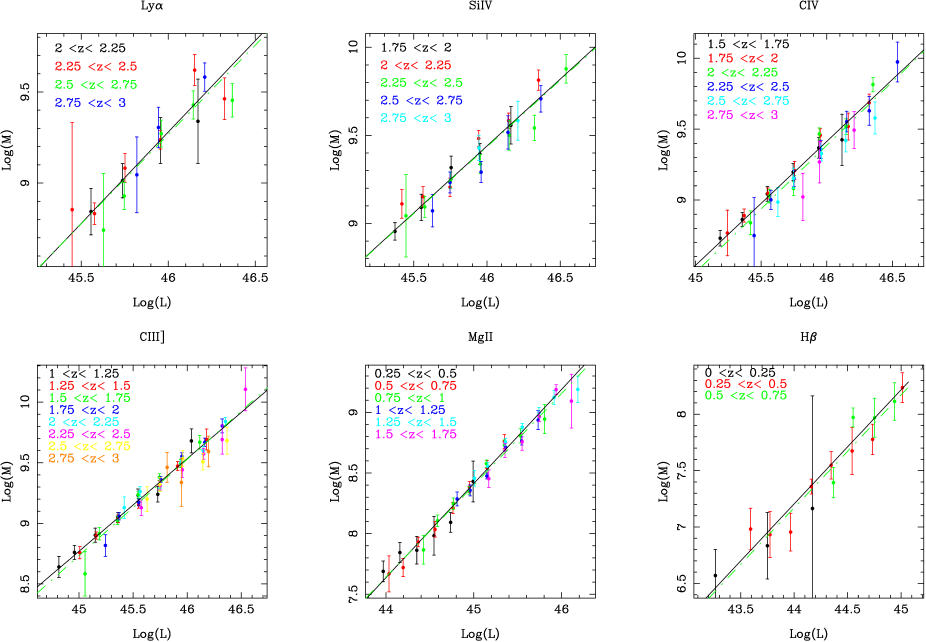
Figure 3: The mass ($M$)–luminosity ($L_{5100}$) relationship for the different broad emission lines. Mass is given in units of $M_{\sun}$ and luminosity in erg s^-1. Different colours reflect the different redshift ranges as shown in the key for each plot and the error bars shown have been scaled such that $\chi^{2}$ is equal to the number of degrees of freedom. The YonX (solid black line) and BCES (green dot-dash line) fits to the $M_{\rm BH}-L$ relationship for each line are also shown.

In reverberation mapping studies (e.g. Wandel et al. 1999, Onken & Peterson 2002) the rms spectrum of the H$\beta$ emission line is often used to estimate the velocity dispersion of the gas. The rms spectra, formed from the rms difference between the individual spectra obtained during the monitoring programme and the mean spectrum, measures only the components which vary and, since the emission from the NLR does not vary significantly on short time scales it should not be present in the rms spectrum. At first sight it therefore seems reasonable that the velocity dispersion of the BLR gas would be best represented by the H$\beta$ velocity width measured from the line after subtraction of the narrow emission line component. However, K00 found that there was little difference between the H$\beta$ line width obtained from the rms spectrum and that measured from the mean spectrum without correcting for the narrow line emission. Vestergaard (2002) also found that the width of the H$\beta$ line in the rms spectrum was more similar to that of a single-epoch observation before any correction for NLR emission. This implies that much of the narrow core of the H$\beta$ emission line (Figure 1) is from gas associated with the BLR (rather than the NLR) and we therefore use the H$\beta$ line width from the composite spectra before correction for any narrow line emission in the analysis which follows. For the non-Balmer lines, we use the FWHM line widths measured after contaminating emission has been subtracted.

A secondary issue is the underlying Fe II emission. As discussed in Section 3.1, many of the Fe II emission features have been treated as continuum, particularly the large feature underlying Mg II, and it is therefore not possible for us to correct the emission lines for the underlying Fe II. This may impact on our measurement of the Mg II FWHM. In their study, McLure & Jarvis (2002) used Mg II FWHM measurements from spectra taken with the International Ultraviolet Explorer (IUE) which had been corrected for the underlying Fe II emission. They found a linear almost one-to-one, correlation between the FWHM measured for the H$\beta$ and Mg II lines whereas we find that the Mg II emission is generally broader than the H$\beta$ emission. On the other hand, some of the H$\beta$ FWHM measurements used by McLure & Jarvis (2002) have been corrected for narrow H$\beta$ emission and in these cases it is reasonable to asume that their H$\beta$ FWHM would be broader than ours.

There is also an Fe II emission line to the red of H$\beta$ ($\sim$ 4930 Å, see e.g. Vanden Berk et al. 2002) which we have not removed before measuring the H$\beta$ FWHM. Vestergaard (2002) found that it was not necessary to correct for the FeII emission unless the FeII emission from the object was unusually strong, and as there is no evidence for strong Fe II emission in our composite spectra, we do not believe this feature will have a significant impact on the H$\beta$ FWHM. In any case, we note that K00 did not correct for Fe II emission when measuring the H$\beta$ FWHM from their mean spectra.

Having determined which measurements of the line widths most accurately represent the velocity dispersion of the gas, we need to obtain an estimate of the radius of the BLR. From reverberation mapping experiments, K00 found the BLR radius, $r\propto$ $L^{0.7}_{5100}$ where $L_{5100}$ is the continuum luminosity at 5100Å (defined as $\lambda L_{5100}$ in K00 and $=3.56\rm{L}_{b}$ for our data). This result depends on the cosmology assumed and the analytic method used to determine the fit. K00 assumed $q_{0}=0.5$, $\lambda_{0}=0$ and $H_{0}=75$ km s^-1 Mpc^-1 and used the fitexy linear regression method (Press et al. 1992), which takes into account errors in both $L$ and $r$, to fit their data. Re-analysing the K00 data, assuming the cosmology adopted here ($\Omega_{0}=0.3$, $\lambda_{0}=0.7$ and $H_{0}=70$ km s^-1 Mpc^-1), Netzer (2003) finds a similar relationship with

$$r=27.4(\frac{L_{5100}}{10^{44}{\rm erg~{}s^{-1}}})^{0.68\pm 0.03}~{}~{}{\rm light~{}days}.$$ (2)

Using the BCES bisector method (Akritas & Bershady 1996) to fit the same data, Netzer (2003) obtains a somewhat flatter relationship, $r\propto L_{5100}^{0.58\pm 0.12}$, although the two fits are formally consistent. Similar results are obtained by McLure & Jarvis (2002) who find $r\propto L_{5100}^{0.61\pm 0.10}$ for our cosmology and the BCES bisector method. Here we have adopted $r\propto L_{5100}^{0.68}$ (Equation 2) but we note that a flatter $r--L_{5100}$ relationship will yield smaller black hole masses at higher luminosities.

The black hole mass is then given by (K00):

$$M_{\rm BH}=1.456\times 10^{5}(\frac{r}{\rm{light~{}days}})(\frac{v}{1000{\rm km~{}s^{-1}}})^{2}M_{\sun}$$ (3)

where $v$ is the FWHM of the H$\beta$ emission line. The BLR clouds are assumed to be in random orbits about the black hole and thus in Equation 3 the velocity dispersion is assumed to be $(\sqrt{3}/2)v$ (Netzer 1990). If the orbits of the BLR clouds are not random but confined to disks, as suggested by e.g., Young et al. 1999, McLure & Dunlop (2002), the velocity dispersion is $(3/2)v$, and the black hole masses are a factor of 3 larger than we derive.

The black hole masses for selected lines were estimated using Equations 2 and 3 and are shown in Figure 3 plotted against $L_{5100}$. As expected, a strong correlation can be seen between BH mass ($M$) and the luminosity, $L_{5100}$, for each line with remarkably little scatter, generally less than 0.3 dex. The best fit of the form $\log(M)=a+\beta\log(L)$ for each line is shown in Figures 3 and 4 with the parameters for each fit given in Table 4. The data were fitted using both the standard linear regression method (YonX) and the BCES method. From Table 4 it is clear that the two methods agree to within the errors (see also Figure 3). For the linear regression method the errors in the fit parameters were evaluated as described in the previous section, using the $\chi^{2}$ of the fit to derive the errors in the mass estimate and hence $a$ and $\beta$. We note that the linear relationship between $M_{\rm BH}$ and $L_{5100}$ derived for the H$\beta$ line is similar to that obtained for the Ly$\alpha$ emission line in this analysis. Fits to the other emission lines are slightly offset from, and flatter than, the fit to the hydrogen lines (Figure 4). Nevertheless, for a given continuum luminosity, the black hole masses obtained from the different emission lines typically lie within $\pm 0.3$ dex of each other.

Table 4: The best fits to the relationship between the black hole mass, $M$, with the monochromatic luminosity, $L_{5100}$, in units of erg s^-1. Black hole mass is in units of $M_{\sun}$. A linear fit of the form $log(M)=a+\beta log(L_{5100})$ was applied to the data, where $\beta$ is the slope of the relationship and $a$ is a constant. $\delta$ is the normalisation constant applied to the data to force the weighted mean of the line to lie on the H$\beta$ YonX relationship and has errors of $\sim$ 0.1dex

Line	method	$a$	$\sigma_{a}$	$\beta$	$\sigma_{\beta}$	$\delta$
Ly$\alpha$	YonX	$-$36.79	4.32	1.00	0.09	$-$0.06
	BCES	$-$35.82	5.08	0.98	0.11
Si IV	YonX	$-$25.49	1.82	0.76	0.04	$-$0.24
	BCES	$-$25.38	1.75	1.02	0.12
C IV	YonX	$-$30.85	1.93	0.87	0.04	$-$0.22
	BCES	$-$31.90	1.86	0.90	0.04
C III]	YonX	$-$25.65	1.17	0.76	0.03	$-$0.38
	BCES	$-$27.09	1.45	0.80	0.03
Mg II	YonX	$-$26.54	0.80	0.78	0.02	$-$0.15
	BCES	$-$25.71	0.88	0.76	0.02
H$\beta$	YonX	$-$37.12	3.32	1.01	0.08	0.0
	BCES	$-$36.90	2.81	1.00	0.06
all data	YonX	$-$32.05	0.08	0.90	0.00
	BCES	$-$33.53	0.78	0.93	0.02
H$\beta$ and	YonX	$-$36.68	0.08	1.00	0.00
C IV only	BCES	$-$36.77	0.74	1.00	0.02

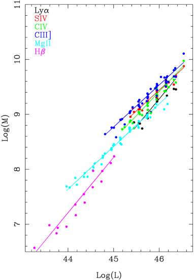
Figure 4: The mass ($M$)–luminosity ($L_{5100}$) relationship for selected broad emission lines, each line shown in a different colour. The best BCES fit to the $M_{\rm BH}-L$ relationship for each line is also shown. Error bars are not plotted for clarity.

Reverberation mapping experiments (e.g., Peterson & Wandel 1999, 2000; Onken & Peterson 2002) find that different emission lines respond to changes in the UV continuum with different time lags. This indicates that the BLR is stratified, with the broader emission lines (such as C IV) originating closer to the central engine than the Balmer lines. The empirical $r-L_{5100}$ relationship (Equation 2) was obtained by K00 from the H$\beta$ and H$\alpha$ emission lines and thus its use to determine black hole masses via Equation 3 will lead to an overestimate of the black hole mass for C IV. To obtain more reliable estimates of $M$ for the UV lines it is necessary to introduce a “calibration” factor to equation 2 to correct for the difference between the radius of the gas emitting the broad UV lines, such as C IV, and that emitting the H$\beta$ lines. This has already been attempted by Vestergaard (2002) who compared the BH masses estimated from reverberation mapping of the H$\beta$ emission line with those estimated from the C IV FWHM in the same object assuming that, for the C IV line,

$$M_{\rm BH}=a(\frac{FWHM_{C{\small~{}IV}}}{1000\rm{km~{}s^{-1}}})^{2}(\frac{L_{1350}}{10^{44}\rm{erg~{}s^{-1}}})^{0.7}$$ (4)

where $L_{1350}$ is the continuum luminosity at 1350Å (i.e. $\lambda$L₁₃₅₀ in Vestergaard 2002) and $a$ is a constant. She found $a=10^{6.2\pm 0.45}$ which implies that the radius of the C IV emission, $r_{C{\small~{}IV}}\sim 0.5^{+1.1}_{-0.4}r_{H\beta}$ (assuming that the QSO spectra have a spectral index of $-0.5$) although the errors in $a$, and hence this result, are large.

To determine the calibration factor for our data we re-normalised the mass-luminosity relationship so that the weighted mean of the mass derived from each line lies on the H$\beta$ (YonX) relation, noting that an extrapolation of the H$\beta$ mass-luminosity relation to higher luminosities is entirely consistent with that observed for Ly$\alpha$. However, because our estimates of black hole mass are based on the underlying assumption that the K00 radius-luminosity relation $r\propto L^{0.68}$ holds for all emission lines, we chose not to adjust the slopes of the observed mass-luminosity relation for each emission line. The mass-luminosity relationships were therefore normalised by the addition of a constant offset, $\delta$ (Table 4). Assuming that this offset is due to the emission lines being emitted from gas situated at different radii, $\delta$ can be converted to provide an estimate of the radius at which the UV lines are emitted relative to that of the H$\beta$ emission (radius = $10^{\delta}r_{\rm{H}\beta}$). We find that the $r_{C{\small~{}IV}}=0.6^{+0.2}_{-0.1}r_{\rm{H}\beta}$ (Table 4) which is consistent with that found by Vestergaard (2002). From their reverberation mapping study of NGC 3783, Onken & Peterson (2002) also find that the C IV emission line lag is approximately half that of the H$\beta$ line although the errors on this measurement are also large.

The calibration factor $\delta$ does not address the variation in the slopes of the mass–luminosity relationships for the different lines, which, if significant, must result from a difference in the measured line width-luminosity relation for different species. Since it is difficult to see how different emission lines could give rise to a different mass–luminosity relations (a line-independent quantity) based on the same set of QSO composite spectra, the most straightforward interpretation of this observation is that the different slopes are caused by the contaminating emission blended with the lines. As we have already discussed in this and previous sections, the Mg II and C III] emission lines are blended with emission from other elements (Fe II and Si III] respectively) which would effectively broaden the measured FWHM of the lines, making our calculation of $\delta$ unreliable. The blended emission could also alter the slope of the $\log(v)-\log(L)$ relation, particularly if the relative contribution of the lines vary with luminosity or redshift. We note that the slope of the $\log(M)-\log(L)$ relationship for H$\beta$ and C IV are statistically identical given their errors (Table 4) and that these lines also suffer the least amount of contamination. We cannot, however, rule out the possibility that the radius-luminosity relation may differ slightly from line to line.

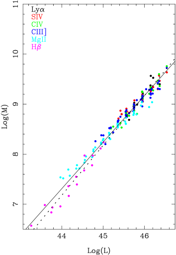
Figure 5: The mass ($M$)–luminosity ($L_{5100}$) relationship for the different lines normalised to the H$\beta$ relationship. Each colour corresponds to a different line. The best BCES fit to the data as a whole is shown (solid line) as well as that to the H$\beta$ and C IV lines alone (dotted line). Error bars are not plotted in the interests of clarity.

The re-normalised mass-luminosity relations for all lines are plotted in Figure 5 and we fit an overall mass-luminosity relation of the form:

$$\log(M_{\rm BH})=0.93(\pm 0.05)\log(L_{5100})-33.5(\pm 2)$$ (5)

to all emission lines (solid line, Fig 5). However, mindful the problems associated with contaminating emission, we also fit a mass-luminosity relation to the H$\beta$ and C IV emission lines only (Fig.5; dotted line) since these lines are the least affected by contaminating emission and should therefore give the most reliable estimate. For the H$\beta$ and C IV lines alone, we find

$$\log(M_{\rm BH})=1.00(\pm 0.1)\log(L_{5100})-36.8(\pm 4.5)$$ (6)

which is slightly steeper than that found for all the emission lines combined.

The errors on the $M_{\rm BH}-L$ relations are larger than those quoted in Table 4. In estimating the errors on these relations we have taken into account the errors on the initial fit to H$\beta$ which, since it is used to normalise the mass estimates from the other emission lines, contributes to the overall errors on the $M_{\rm BH}-L$ relation. The error in the fit to the H$\beta$ and C IV lines is larger than that obtained for all the emission lines as we have fewer data points. Note the errors on the gradient and the intercept in Equation 5 and 6 are not independent and have a correlation of nearly -1. The relations we obtain are in reasonable agreement with the statistical analysis of Netzer (2003), who finds $M_{\rm BH}\propto L^{0.9\pm 0.15}_{1350}$ for $r_{\rm BLR}\propto L^{0.68}_{1350}$ (where $L_{1350}$ is the luminosity at 1350Å) for a sample of over 700 objects (Table 1; Netzer 2003).

An important caveat on the $M_{\rm BH}-L$ relationship given in equations 5 and 6 is that throughout our analysis we have used the relationship $r_{\rm BLR}\propto L^{\gamma}_{5100}$ discovered by K00 and later refined by McLure & Jarvis (2002) and Netzer (2003). As discussed previously, the value of $\gamma$ is uncertain and depends on the statistical method used to fit the data, with the fitexy method and the BCES method giving values of $0.68\pm 0.03$ and $0.58\pm 0.12$ respectively for the same data. Although there is a correlation between velocity and luminosity (Section 4) the slope of the $\log(v)=a+b\log(L_{5100})$ relationship is quite flat for most of the emission lines (e.g, $b=0.17$ for H$\beta$, 0.1 for C IV, 0.05 for Mg II; Table 3) and the slope of the $\log(M_{\rm BH})-\log(L_{5100})$ relation is therefore dominated by the value assumed for $\gamma$ which is currently known to an accuracy of only $\pm 0.15$. For example, if we adopt $\gamma=0.58$ in Equation 2, we find $M_{\rm BH}\propto$ $L^{0.83}_{5100}$ for all lines and $M_{\rm BH}\propto$ $L^{0.9}_{5100}$ for the H$\beta$ and C IV lines alone, again consistent with Netzer (2003).

Additionally, and perhaps more importantly, it is not known whether $\gamma$ is constant across all luminosity ranges. The sources in K00’s sample all have $L_{5100}<10^{46}$ erg s^-1, with only 4 (out of a total sample of 34) having $L_{5100}>10^{45}$ erg s^-1. Our mass estimates for the UV lines are therefore based on the assumption that the $r_{\rm BLR}\propto L_{5100}$ relation can be safely extrapolated to higher luminosities. Netzer (2003) found that eliminating the 3 objects with $L_{5100}<10^{43}$ erg s^-1 from K00’s sample resulted in a $\gamma(BCES)=0.71\pm 0.21$ and $\gamma(fitexy)=0.69\pm 0.03$ whereas eliminating the seven objects with $L_{5100}<10^{43.7}$ erg s^-1 resulted in $\gamma(BCES)=0.58\pm 0.19$ and $\gamma(fitexy)=0.74\pm 0.04$. Reverberation mapping of multiple line species in the same object and extending the luminosity range of reverberation mapped sources would clearly be of great benefit in eliminating some of uncertainties with this analysis.

5.2 Narrow emission lines and black hole masses

A number of studies have found that the stellar velocity dispersion of the host galaxy bulge is related to the bulge luminosity which is, in turn, related to the mass of the black hole (e.g. Magorrian et al. 1998; Ferrarese et al. 2001; Tremaine et al. 2002). Recently, Shields et al. (2002) and Boroson (2003) investigated the possibility of using the velocity width of [O III] as a substitute for the stellar velocity dispersion when determining the black hole mass. They both found that the velocity width of [O III] is correlated with black hole mass, assuming that the black hole mass $\propto$ $L^{\gamma}v^{2}$ where $L$ is the QSO luminosity at 5100Å, $v$ is the velocity width of the H$\beta$ emission line and $\gamma=0.5$ and 0.7 for Shields et al. (2002) and Boroson (2003) respectively. We find that the velocity width of [O III] is correlated with the luminosity of the QSO (Table 1) with $v\propto L^{0.1\sim 0.15}$ (Table 3; FWHM values as the IPV values are probably contaminated by Fe II emission either side of the [O III] lines), similar to that found for H$\beta$. This raises the intriguing possibility first, that the NLR in QSOs is sufficiently close to the black hole for its motion to be dominated by the gravitational potential of the black hole, and secondly, that the narrow emission lines may be used to derive the black hole mass. However, none of the other narrow emission lines in our study ([O II], [Ne V] and [Ne III]) display the same strength of correlation between line width and QSO luminosity as [O III] and given the anti-correlation between narrow line strength and continuum luminosity (Croom et al. 2002) the use of narrow lines in estimating the black hole mass may be limited to low luminosity and hence low mass objects.

5.3 Evolution of the black hole mass-to-luminosity ratio

Figure 3 shows the mass–luminosity relation for the individual broad lines separated into redshift bins and appears to demonstrate a lack of evolution in the relation between black hole mass and luminosity with redshift. However, the C IV line does show a significant anti-correlation between velocity and redshift in our partial correlation analysis (Table 2) which may be evidence of a weak redshift evolution of line width. No other lines show significant correlations with redshift.

In order to make a quantitative estimate of the amount of redshift evolution we fit a simple power law model to the $L-z$ data points for each emission line. We first assume that black hole mass is related to luminosity and redshift by independent power laws such that

$$M_{\rm BH}(z)\propto L(z)^{\alpha}(1+z)^{\beta},$$ (7)

and that secondly, the radius-luminosity relation is also described by a power law:

$$R\propto L(z)^{\gamma}.$$ (8)

We assume that the radius-luminosity relation (Equation 8) does not to evolve with redshift as it should be primarily driven by the physics of photoionization, which we would not expect to change with redshift (although this may not be the case if QSO metallicity was found to evolve). Assuming Keplerian motion, we have

$$\log(v)=\frac{\alpha-\gamma}{2}\log(L)+\frac{\beta}{2}\log(1+z)+Const.$$ (9)

This relation is then fitted to the observed velocity-luminosity data for each emission line individually (as we do not wish to assume that the radius-luminosity relation is the same for each emission line). To obtain a more realistic estimate of the errors on the fitted parameters given a large intrinsic scatter in the data, we re-scale the errors on individual points such that $\chi^{2}$ is equal to the number of degrees of freedom. The results of this model fitting are shown in Table 5. The only line which shows clear evidence ($>3\sigma$) for evolution is C IV. However, Si IV and C III] also show weak evolution in the same sense. All of these lines have best fit values of $\beta$ which are negative, implying that for a given luminosity, the measured velocities are lower at higher redshift. By contrast, the value of $\beta$ for the Mg II line is entirely consistent with no evolution at all and the Balmer lines (H$\beta$ and H$\gamma$) all show positive values of $\beta$, although these are not significant. We do not attempt to model the redshift evolution of the Ly$\alpha$ line, as the contribution of Ly$\alpha$ forest absorption and N V emission makes any interpretation highly uncertain. To show more clearly the evolution in the C IV velocity width, we plot $\log(v)$ vs. $\log(1+z)$ for this line, first renormalizing the velocity points to a constant absolute magnitude (based on the above fits) of $M_{\rm B}=-25.0$ (Fig. 6). The error bars in Fig. 6 have been rescaled such that $\chi^{2}$ is equal to the number of degrees of freedom. A weak, but significant, decline in velocity can be seen, particularly at $\log(1+z)>0.5$.

Figure 6: The evolution of C IV velocity width. We plot the re-normalized (to a fixed absolute magntude of $M_{\rm B}=-25.0$) velocity vs. $(1+z)$ in log-log space. The error bars have been re-scaled such that $\chi^{2}$ is equal to the number of degrees of freedom. A decline in velocity can be seen at the highest redshifts.

The evolution seen in the higher redshift lines is in the sense of higher redshift QSOs having smaller velocities for the same luminosities, which might be expected if QSO luminosity evolution is driven by a decline in fueling rate at lower redshift. However, the amount of evolution is small compared to the strong luminosity evolution shown by QSOs (typically $\sim(1+z)^{3}$). At $z\sim 2-3$ the QSO evolution slows down and appears to turn over. Assuming pure luminosity evolution (PLE), Croom et al. (2003) finds that for the full 2QZ catalogue the evolution of $L^{*}$, the characteristic luminosity of the QSO population, is well described by $L^{*}(z)=L^{*}(0)10^{k_{1}z+k_{2}z^{2}}$ with $k_{1}=1.17$ and $k_{2}=-0.21$ at redshifts less that $z\sim 2.3$. This model implies that $L^{*}$ reaches an extrapolated maximum at $z\sim 2.8$. If black hole masses do not evolve, and the luminosity evolution is purely due to other influences (e.g. fueling rate), then at a given luminosity $M_{\rm BH}(z)=M_{\rm BH}(0)$. Thus, using the PLE fit from Boyle et al (2003) and assuming that $M\propto L^{\alpha}$ we find

$$\frac{M_{\rm BH}(z)}{L^{\alpha}(z)}=\frac{M_{\rm BH}(0)}{L^{\alpha}(0)}10^{-\alpha(k_{1}z+k_{2}z^{2})}.$$ (10)

In Figure 7 we compare this model to the evolutionary slopes found in our fits. Our PLE model (solid line) is steep at low redshift, but flattens off at $z\sim 2-3$. Here we assume that $\alpha=0.93$, as found in Section 5.1 for all broad emission lines, but the shape of the model curve changes little if $\alpha=1.0$, as found for the H$\beta$ and C IV lines alone (Section 5.1). We plot, as shaded regions, the range of allowable ($\pm 1\sigma$) slopes for each of five lines (H$\beta$, Mg II, C III], C IV and Si IV), over the redshift ranges that they are measured. Each is normalized to the $M(z)/L^{\alpha}(z)$ ratio at the mean redshift of the line. At low redshift, the H$\beta$ line has a positive slope which is consistent with $\beta=0$, but not with the strong evolution of the model (solid line). At higher redshift the Mg II and C III] lines are close to $\beta=0$ and although this is inconsistent with our model, we note that both these lines are contaminated by blended emission which could be distorting their behaviour. Only the highest redshift lines, C IV and Si IV show evolution which is comparible to that shown by the model, partly as they have higher values of $\beta$ and partly as the model starts to turn over at high redshift.

Figure 7: The best fit evolutionary power law relationships. The evolution predicted by the luminosity evolution of Boyle et al. (solid line) is compared to the slopes found in our fits (shaded regions). The horizontal width of the individual shaded regions represents the redshift range covered by our data for each emission line and the height of the regions represents the $1\sigma$ error on $\beta$ (Table 5). The vertical positioning of the shaded regions is such that they intersect the model at their mean redshift (see text for a more detailed discussion).

Table 5: The best fit evolutionary power law slopes.

Line	$\beta$	$\Delta\beta$
Si IV	$-$0.76	0.36
C IV	$-$0.86	0.25
C III]	$-$0.23	0.12
Mg II	0.00	0.18
H$\gamma$	0.84	1.85
H$\beta$	0.94	2.23

It appears that only at $z>2$ does the measured evolution in the luminosity-velocity relation compare to the above model. Over the majority of the redshift range covered in this investigation evolution in the luminosity-velocity relation is insignificant. This conclusion has significant implications for QSO evolution, implying little evolution in the mass-luminosity relation for super-massive black holes over a wide range in redshift. Assuming no evolution in the mass-luminosity relation we can transform the QSO luminosity function (LF) and its evolution with redshift into a mass function (MF). In Fig. 8 we show the evolution of the QSO mass function based on the LF derived from the 2QZ+6QZ samples (Croom et al. 2003). We immediately note that the luminosity (mass) evolution of the QSO LF cannot be explained by decline in the fueling rate – either in continuous model (long-lived QSOs) or in a duty cycle (short-lived QSOs), since this would imply that a QSO at a given relative position on the LF (MF) evolving from high black hole mass at high redshift to low black hole mass at low redshift.

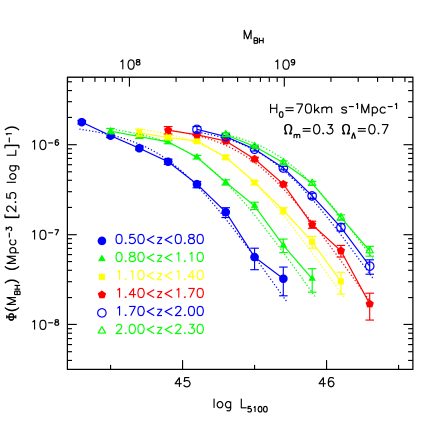
Figure 8: The Black Hole Mass Function for QSOs and its evolution with redshift.

Rather, the evolution of the black hole mass function suggests that QSOs can only be active once, possibly associated with formation of the black hole itself during spheroid formation. Under this interpretation, the evolution of the LF is driven by the efficiency of black hole formation which drops rapidly towards low redshift. This picture is qualitatively consistent with the recent theoretical work of Kauffmann & Haehnelt (2000), although it places tight constraints on the fraction of QSOs which exhibit a duty cycle of activity in such models.

It also implies that the Gebhardt et al. (2002) relation between black hole mass and galaxy velocity dispersion will evolve toward higher ratios at higher redshifts. The black hole mass will be ’frozen’ when black hole formation and subsequent QSO activity ceases while the mass/velocity dispersion of the host galaxies will increase due to hierarchical merging to give the relationship seen at the present day.

At $z\sim 2$ and greater, there does seem to be some evolution of the velocity-luminosity relation, as shown by the C IV (Fig. 6) and Si IV lines. It appears that there is a general decline in velocity for a given luminosity at $\log(1+z)>0.5$ ($z>2.2$). The measured rate of evolution is no different if we remove the highest redshift bin ($2.75<z<3.0$) and re-fit the data. The fact that the strongest evolution in the velocity-luminosity relationship is found in the redshift regime corresponding to the peak of QSO activity suggests that as $L^{*}$ declines at high redshift ($z>2.5$), the black hole mass-luminosity relation may be changing more rapidly than at lower redshift.

6 Conclusions

We have used composite spectra generated from more than 22000 QSOs observed in the course of the 2dF and 6dF QSO redshift surveys to investigate the relationship between the profiles of emission lines and luminosity. We find that the velocity width of the broad emission lines H$\beta$, H$\gamma$, Mg II, C III] and C IV show a positive correlation with the continuum luminosity (as measured in the $b_{{\rm J}}$ filter) but the slope of this dependence is much flatter for the UV emission lines (Mg II, C III] and C IV ) than for the hydrogen lines. This correlation is statistically significant with a confidence level $>99$ per cent and is independent of the method used to measure the emission line widths. From partial Spearman correlation analysis we find only weak evidence for an anti-correlation between redshift and velocity. Of the narrow emission lines, [O II], [Ne III], [Ne V] and [O III], only the [O III] $\lambda$5007 line exhibits a correlation between line width and luminosity.

Assuming that the gas in the BLR is in near-Keplerian orbits and that the radius of the BLR, $r\propto L^{0.68}$ (K00;Netzer 2003), where $L$ is the continuum monochromatic luminosity at 5100Å, we have used our measurements of the emission line velocity widths to derive estimates of the average black hole mass in the composite spectra. We find that for a given luminosity the black hole masses obtained from the different the emission lines agree to within 0.6dex. However the scatter in the mass-luminosity relationships for the individual lines is much smaller ($<0.3$ dex) and given that the different emission lines may be emitted from different radii, producing an offset between the masses estimated from different emission lines, we use the H$\beta$ $M_{\rm BH}-L$ relationship to calibrate the other emission lines. We find an overall black hole mass - luminosity relationship of the form $M_{\rm BH}\propto L^{0.93\pm 0.05}$. It is possible that the FWHM measurements of several of the emission lines are overestimated as they are blended with weaker lines from different elements which are difficult to remove reliably. We have therefore also derived the mass–luminosity relationship for the H$\beta$ and C IV emission lines only, as these are the lines least effected by contaminating emission, and find $M_{\rm BH}\propto L^{1.0\pm 0.1}$. Our$M_{\rm BH}-L$ relationships depend heavily on the slope of the $\log(r)-\log(L)$ relationship which is currently known to an accuracy of only $\pm 0.15$. Using the midpoint of the derived $M_{\rm BH}-L$ powerlaws and taking into account the error in the slope of the $\log(r)-\log(L)$ relationship, we conclude that $M_{\rm BH}\propto L^{0.97\pm 0.16}$.

We find only weak evidence of evolution in the velocity-luminosity correlation, which places strong constraints on the evolution of black hole masses for a fixed QSO luminosity; $M\propto(1+z)^{\beta}$, $\beta<1$. This is much smaller than that required for the luminosity (mass) function of QSOs to be due to a single population of long-lived sources.

References

- [Akritas & Bershady] Akritas M.G., Bershady M.A., 1996, ApJ, 470, 706
- [Baldry et al. 2002] Baldry I. K. et al, 2002, ApJ, 569, 582
- [Baldwin 1977] Baldwin J. A., 1977, ApJ, 214, 679
- [Blanford & McKee 1982] Blanford R.D., McKee C. F. 1982, ApJ, 255, 419
- [Boroson & Green 1992] Boroson T. A., Green R. F., 1992, ApJ, 80, 109
- [Boroson 2003] Boroson T. A., 2003, ApJ in press (astro-ph/0211372)
- [Boyle et al. 2000] Boyle B. J., Shanks T., Croom S. M., Smith R. J., Miller L., Loaring N., Heymans C., 2000, MNRAS, 317, 1014
- [Boyle 1990] Boyle B. J., 1990, MNRAS, 243, 231
- [Boyle et al. 1988] Boyle B. J., Shanks T., Peterson, B. A., 1988, MNRAS, 235, 935
- [Cristiani & Vio 1990] Cristiani S., Vio R., 1990, A&A, 227, 385
- [Croom et al. 2001] Croom S. M., Smith R. J., Boyle B. J., Shanks T., Loaring N. S., Miller L., Lewis I. J., 2001, MNRAS, 322, L29
- [Croom et al. 2002] Croom S. M., Rhook K., Corbett E. A., Boyle B. J., Netzer H., Loaring N. S., Miller L., Outram P. J., Shanks T., Smith R. J., 2002, MNRAS, 337, 275
- [Croom et al. 2003] Croom et al. 2003, in preparation
- [Ferrarese et al. 2001] Ferrarese L., Podge R. W., Peterson B. M., Merritt D., Wandel A., Joesph, C. L., 2001, ApJ, 555, L79
- [Francis et al. 1991] Francis P. J., Hewett P. C., Foltz C. B., Chaffee F. H., Weymann R. J., Morris S. L., 1991, ApJ, 373, 465
- [Gebhardt et al. 2000] Gebhardt K., et al. 2000,ApJ,543, L5
- [Green et al. 2001] Green P. J., Forster K., Kuraszkiewicz J., 2001, ApJ, 556, 727
- [Joly et al. 1985] Joly M., Collin-Souffrin S., Masnou J.L., Nottale L., 1985, A&A, 152, 282
- [Kaspi et al. 1996] Kaspi S., Smith P. S., Maoz D., Netzer H., Jannuzi B. T., 1996, ApJ, 471,L75
- [Kaspi et al. 2000] Kaspi S., Smith P. S., Netzer, H., Maoz, D., Januzzi B. T., Giveon U., 2000, ApJ, 533, 631 (K00)
- [Kauffman & Haehnelt 2000] Kauffman G., Haehnelt G., 2000, MNRAS, 311, 576
- [Krolick 2001] Krolick J., ApJ, 551, 72
- [Magrorrian et al. 1998] Magorrian J., et al. 1998, AJ, 115, 2285
- [Moaz 2002] Maoz, D. 2002 astro-ph/0207295
- [Miyoshi et al. 1995] Miyoshi M., Moran J., Hernstein J., Greenhill L., Nakai N., Diamond P., Inoue M., 1995 Nature, 373, 127
- [McLure & Dunlop 2002] McLure, R. J., Dunlop, 2002, MNRAS, in press
- [McLure & Jarvis 2002] McLure, R. J., Jarvis, M. J., 2002, MNRAS, in press
- [Netzer 1990] Netzer H., 1990 in Active Galactic Nuclei, Saas Fee Advanced Course 20, ed. T. J. -L. Courvoisier & M. Major (Berlin:Springer), 57
- [Netzer 2003] Netzer H., 2003, ApJ, 583 L5
- [Onken & Peterson 2000] Onken C. A., Peterson B.M. 2002, ApJ, 572, 746
- [Peterson & Wandel 1999] Peterson B. M., Wandel A., 1999, ApJ, 521, L95
- [Peterson et al. 2000] Peterson B. M., et al., 2000, ApJ, 542, 161
- [Press et al. 1992] Press W. H., Teukolsky S.A., Vetterling W.T., Flannery B.P., 1992, Numerical recipes (Second ed,; Cambridge: Cambridge Univ. Press), 660
- [Robinson 1995] Robinson, A., MNRAS, 272, 647
- [Schlegel et al. 1998] Schlegel D.J., Finkbeiner D.P.,Davis M., 1998, ApJ, 500 525
- [Smith et al. 2002] Smith J.E, Robinson A., Young S., Corbett E.A., Axon D.A., Gianuzzi M.E., 2002, MNRAS, in press
- [Stirpe 1991] Stirpe G., 1991, A&A, 247, 3
- [Stirpe et al. 1999] Stirpe G., Robinson A., Axon D. J, 1999, in Structure and Kinematics of Quasar Broad Line Regions, ed. C. M. Gaskell, W. Brandt, M. Dietrich, D. Dultzin-Hacyan, Eracleous, 175, p. 249
- [Shields et al. 2002] Shields G. A., Gebhardt K., Salviander S., Wills B. J., Xie B., Brotherton M.S., Yuan J., Dietrich M., 2002, ApJ submitted (atsro-ph/0210050)
- [Tanaka et al. 1995] Tanaka Y., et al. 1995, Nature, 375, 659
- [Tremaine et al. 2002] Tremaine et al., 2002, ApJ, 574, 740
- [Wandel et al. 1999] Wandel, A., Peterson, B. M., Malkan, M. A., 1999, ApJ, 526, 579
- [Wandel & Yahil 1985] Wandel, A., A., 1985, ApJ, 295, L1
- [Whittle 1985] Whittle,1985, MNRAS, 213, 1
- [Wilms et al. 2001] Wilms J., Reynolds C. S., Begelman M. C., Reeves J., Molendi S., Staubert R., Kendziorra E., 2001, MNRAS, 328 L27
- [Woo & Urry 2002] Woo J. H., Urry C. M., 2002, ApJ, 579, 530
- [Young et al. 1999] Young S., Corbett E.A., Hough J.H., Gianuzzi M.E., Robinson A., 1999, MNRAS
- [Vestergaard 2002] Vestergaard, M. 2002, ApJ, 571, 733