Anthropic predictions for neutrino masses

Abstract

It is argued that small values of the neutrino masses may be due to anthropic selection effects. If this is the case, then the combined mass of the three neutrino species is expected to be $\sim 1$ eV, neutrinos causing a non-negligible suppression of galaxy formation.

I Introduction

The major ingredients of the Universe are dark energy, $\Omega_{\Lambda}\sim 0.7$, and non-relativistic matter, $\Omega_{m}\sim 0.3$. The latter consists of non-baryonic dark matter, $\Omega_{D}\sim 0.25$, baryons, $\Omega_{B}\sim 0.05$, and massive neutrinos, $\Omega_{\nu}\gtrsim 0.001$. The fact that $\Omega_{\Lambda}$ is comparable to $\Omega_{m}$ is deeply puzzling; this is the notorious coincidence problem that has been much discussed in the recent literature. The only plausible explanation that has so far been suggested is that $\Omega_{\Lambda}$ is a stochastic variable and that the coincidence is due to anthropic selection effects. Anthropic bounds on the cosmological constant derived in Davies ; BT ; LindeLambda ; Weinberg87 were followed by anthropic predictions Vilenkin95a ; Efstathiou95 ; Martel98 ; GV suggesting values not far from the presently observed dark energy density. Although controversial, such anthropic arguments have been bolstered by the discovery of mechanisms that may be capable of creating ensembles with different parameter values in the context of both cosmic inflation AV83 ; Linde86 ; Linde90 and string theory Bousso ; Banks ; Donoghue01 ; Susskind03 , and have been applied to other physical parameters as well CarrRees ; Rees79 ; Linde88a ; Linde88b ; Linde95 ; Bellido95 ; Vilenkin95d ; Vilenkin97 ; Q ; dimensions ; t98 ; Agrawal ; Donoghue98 ; Tanaka ; Mario ; Hogan00 ; Aguirre ; multiverse .

Perhaps equally puzzling are the “coincidences” $\Omega_{D}\sim\Omega_{B}$ and $\Omega_{B}\sim\Omega_{\nu}$. These three matter components are relics of apparently unrelated processes in the early Universe, and it is very surprising that their mass densities are comparable to one another. The mass density of neutrinos is $\Omega_{\nu}=(m_{\nu}/94{\rm eV})h^{-2}$, where $m_{\nu}$ is the combined mass of all three neutrino flavors. In this paper, we will investigate the possibility that $m_{\nu}$ is a stochastic variable taking different values in different parts of the Universe and that the observed value is anthropically selected.

Before delving into details, let us briefly outline the argument. A small increase of $m_{\nu}$ can have a large effect on galaxy formation. Neutrinos stream out of the potential wells created by cold dark matter and baryons, slowing the growth of density fluctuations. As a result, there will be fewer galaxies (and therefore fewer observers) in regions with larger values of $m_{\nu}$. If the suppression of galaxy formation becomes important for $m_{\nu}\gtrsim{\tilde{m}}_{\nu}$, say, then values $m_{\nu}\gg{\tilde{m}}_{\nu}$ will be rarely observed because the density of galaxies in the corresponding regions is very low. Moreover, unless the underlying particle-physics model strongly skews the neutrino mass distribution towards values near zero, values $m_{\nu}\ll{\tilde{m}}_{\nu}$ are also unlikely to be observed, simply because the corresponding range of $m_{\nu}$-values is very small. A typical observer thus expects to find $m_{\nu}\sim{\tilde{m}}_{\nu}$, i.e., a mild but non-negligible suppression of galaxy formation by neutrinos.

II Probability distribution for $m_{\nu}$

To make the analysis quantitative, we define the probability distribution ${\cal P}(m_{\nu})dm_{\nu}$ as being proportional to the number of observers in the Universe who will measure $m_{\nu}$ in the interval $dm_{\nu}$. This distribution can be represented as a product Vilenkin95a

$${\cal P}(m_{\nu})={\cal P}_{*}(m_{\nu})n_{obs}(m_{\nu}).$$ (1)

Here, ${\cal P}_{*}(m_{\nu})dm_{\nu}$ is the prior distribution, which is proportional to the comoving volume of those parts of the Universe where $m_{\nu}$ takes values in the interval $dm_{\nu}$, and $n_{obs}(m_{\nu})$ is the number of observers that evolve per unit comoving volume with a given value of $m_{\nu}$. The distribution (1) gives the probability that a randomly selected observer is located in a region where the sum of the three neutrino masses is in the interval $dm_{\nu}$.

Of course we have no idea how to estimate $n_{obs}$, but what comes to the rescue is the fact that the value of $m_{\nu}$ does not directly affect the physics and chemistry of life. As a rough approximation, we therefore assume that $n_{obs}(m_{\nu})$ is simply proportional to the fraction of all baryons that form stars, which we approximate by the fraction $F_{M}(m_{\nu})$ of all matter that collapses into galaxy-scale haloes (with mass greater than $M=10^{12}M_{\odot}$),

$$n_{obs}(m_{\nu})\propto F_{M}(m_{\nu}).$$ (2)

The idea is that there is some average number of stars per unit mass in a galaxy and some average number of observers per star. The choice of the halo mass scale is based on the empirical fact that most stars are observed to be in large halos.

The prior distribution ${\cal P}_{*}(m_{\nu})$ depends on the extension of the particle physics model which allows neutrino masses to vary and perhaps on stochastic processes during inflation which randomize these variable masses. Some candidate prior distributions will be discussed in Section III.

The fraction of collapsed matter $F_{M}(m_{\nu})$ can be approximated using the standard Press-Schechter formalism PressSchechter . We assume a Gaussian density fluctuation field $\delta({\bf x},t)$ with a variance $\sigma(M,t)$ on the galactic scale $(M=10^{12}M_{\odot})$,

$$P(\delta,t)\propto\exp\left[-{\delta^{2}\over{2\sigma(t)^{2}}}\right].$$ (3)

A collapsed halo is assumed to form when the linearized density contrast $\delta$ exceeds a critical value $\delta_{c}$ determined by the spherical collapse model. As detailed in Appendix A, this corresponds to $\delta_{c}\approx 1.69$ around the present epoch and $\delta_{c}\approx 1.63$ in the infinite future Weinberg87 . Using the Press-Schechter approximation, we obtain

$$F_{M}(t)\propto P[\delta>\delta_{c}]=\int_{\delta_{c}}^{\infty}P(\delta,t)d\delta={\rm erfc}\,\left[{\delta_{c}\over\sqrt{2}\sigma_{M}(t)}\right].$$ (4)

The collapsed fraction $F_{M}$ thus grows over time as the rms density fluctuations $\sigma$ increase.

Let us now quantify the effect of neutrino masses on this process. For the small scale $M$ that we are considering, assuming a flat Universe, this fluctuation growth is well approximated by

$$\sigma_{M}(x)\approx\left[1+{3\over 2}A_{\Lambda}(f_{\nu})G_{\Lambda}(x)\right]^{p(f_{\nu})}\sigma_{M}(0),$$ (5)

as shown in Appendix A. The functions $A_{\Lambda}$, $G_{\Lambda}$ and $p$ are defined below. Here we have replaced $t$ by a new time variable

$$x\equiv{\rho_{\Lambda}\over\rho_{\rm m}}={\Omega_{\Lambda}\over(1+z)^{3}\Omega_{\rm m}}={1-\Omega_{\rm m}\over\Omega_{\rm m}}(1+z)^{-3},$$ (6)

i.e., the dark-energy-to matter density ratio — we will consider several values of $x$ below, corresponding to the infinite future ($x=\infty$), the present epoch ($x=7/3$, our default value) and redshift unity ($x=7/24$). The function

$$G_{\Lambda}(x)\approx x^{1/3}\left[1+\left({x\over G_{\infty}^{3}}\right)^{\alpha}\right]^{-1/3\alpha},$$ (7)

where $\alpha=0.795$ and

$$G_{\infty}\equiv{5\Gamma\left({2\over 3}\right)\Gamma\left({5\over 6}\right)\over 3\sqrt{\pi}}\approx 1.43728,$$ (8)

describes how in the absence of massive neutrinos, fluctuations grow as the cosmic scale factor $a$ as long as dark energy is negligible ($G_{\Lambda}(x)\approx x^{1/3}\propto a\propto(1+z)^{-1}$ for $x\ll 1$) and then asymptote to a constant value as $t\to\infty$ and dark energy dominates ($G_{\Lambda}(x)\to G_{\infty}$ as $x\to\infty$).

We are considering the case where $m_{\nu}$ varies from place to place whereas the physics that determined the amount of baryons and cold dark matter per photon is the same everywhere, so the neutrino fraction $f_{\nu}$ is given by

$$f_{\nu}\equiv{\Omega_{\nu}\over\Omega_{\rm m}}={\rho_{\nu}\over\rho_{\rm bc}+\rho_{\nu}}=\left[1+{\rho_{\rm bc}\over\rho_{\nu}}\right]^{-1}=\left[1+{m_{\rm bc}\over m_{\nu}/3}\right]^{-1},$$ (9)

where $\rho_{\rm bc}$ denotes the non-neutrino density, i.e., that of baryons and cold dark matter, and $m_{\rm bc}\approx(4.75\pm 0.30)$eV gives the measured amount of such matter per neutrino. In other words, increasing the neutrino mass from zero will increase the total matter density per photon by a factor $\rho_{\rm m}/\rho_{\rm bc}=(1-f_{\nu})^{-1}$.

$$A_{\Lambda}(f_{\nu})\equiv x_{\rm eq}^{-1/3}=\left({\Omega_{\rm m}\over\Omega_{\Lambda}}\right)^{1/3}(1+z_{\rm eq})$$ (10)

is the factor by which the Universe has expanded between matter-radiation equality at $x=x_{\rm eq}$ (when fluctuations effectively start to grow) and dark energy domination at $x=1$ (when fluctuations gradually stop growing). Since massive neutrinos boost the matter density by a factor $(1-f_{\nu})^{-1}$, they delay vacuum domination until the scale factor is larger by a factor $(1+f_{\nu})^{1/3}$ and also, in the approximation that neutrinos are nonrelativistic at the matter-radiation equality epoch (valid for $m_{\nu}\mathrel{\hbox to0.0pt{\lower 3.0pt\hbox{$\mathchar 536\relax$}\hss}\raise 2.0pt\hbox{$\mathchar 318\relax$}}1$ eV), cause matter-radiation equality to occur occurs earlier, when the scale factor is smaller by a factor $(1+f_{\nu})$. We thus have

$$A_{\Lambda}(f_{\nu})=(1-f_{\nu})^{-4/3}A_{\Lambda}(0).$$ (11)

Finally, neutrinos with nonzero mass suppress the galaxy density through the exponent $p(f_{\nu})$ in equation (5), which is given by Bond80

$$p(f_{\nu})={\sqrt{25-24f_{\nu}}-1\over 4}\approx(1-f_{\nu})^{3/5},$$ (12)

and drops from unity for $f_{\nu}=0$ to smaller values as $f_{\nu}$ increases.

In summary, equation (5) shows that the galaxy fluctuation evolution $\sigma_{M}(x)$ depends on the three cosmological parameters $A_{\Lambda}(0)$, $\sigma_{M}(0)$ and $f_{\nu}$. To study the galaxy density as a function of neutrino fraction $f_{\nu}$ using equation (4), we thus need to measure $A_{\Lambda}(0)$ and $\sigma_{M}(0)$ from observational data without making any assumptions about $f_{\nu}$. We cannot do this using the values of $\Omega_{\rm m}$ and $z_{\rm eq}$ reported by, say, the WMAP team Spergel03 , since these assume that $f_{\nu}=0$ in our part of the Universe; if $f_{\nu}>0$ here, then matter-radiation equality occurred earlier. We therefore repeat the Monte Carlo Markov Chain analysis reported in column 5 of Table 3 in sdsspars , measuring $A_{\Lambda}(0)$ and $\sigma_{M}(0)$ from the WMAP microwave background power spectrum Hinshaw03 combined with the Sloan Digital Sky Survey (SDSS) galaxy power spectrum sdsspower . These measurements are independent of $f_{\nu}$ since this is a free parameter in the analysis and therefore effectively marginalized over. This gives $A_{\Lambda}(0)=3057\pm 502$, $\sigma_{M}(0)\approx 0.000579\pm 0.000064$. The above-mentioned $m_{\rm bc}$-value was measured using this same MCMC analysis. We will use the central values for our main analysis and quantify the effect of the uncertainties in the discussion section. Equation (5) thus shows that for $f_{\nu}=0$, fluctuations grow by a factor $1+1.5A_{\Lambda}(0)G_{\Lambda}(x)\approx 4700$ by the present epoch, which we take to be $x=\Omega_{\Lambda}/\Omega_{\rm m}\approx 0.7/0.3\approx 2.3$, giving $\sigma_{M}\approx 2.7$. In the infinite future $x\to\infty$, fluctuations will have grown by a factor $6600$, giving $\sigma_{M}\approx 3.8$. The basic reason that neutrinos have such a dramatic effect is that these growth factors are so large, implying that even a modest change in the exponent $p(f_{\nu})$ makes a large difference. Taylor expanding equation (5) in $f_{\nu}$ gives

$$\sigma_{M}(x,f_{\nu})\approx\sigma_{M}(x,0)e^{-\gamma(x)f_{\nu}}$$ (13)

for $f_{\nu}\ll 1$, where $\gamma(x)\equiv 0.6\ln[1+1.5A_{\Lambda}(0)G_{\Lambda}(x)]-4/3\approx 3.7$ for the present epoch and $\gamma\approx 3.9$ for the infinite future. Although equation (13) is quite a crude approximation, underestimating the suppression, it shows that small changes in $A_{\Lambda}$ or $x$ are unimportant since they affect this exponential fluctuation suppression only logarithmically.

The effect of neutrino free streaming on the galactic density is illustrated in Fig. 1 (top), which shows that the suppression is non-negligible already for $m_{\nu}\sim 1$ eV. We use equation (5) in our calculations for the plots — the approximation equation (13) was merely to provide qualitative intuition for the effect.

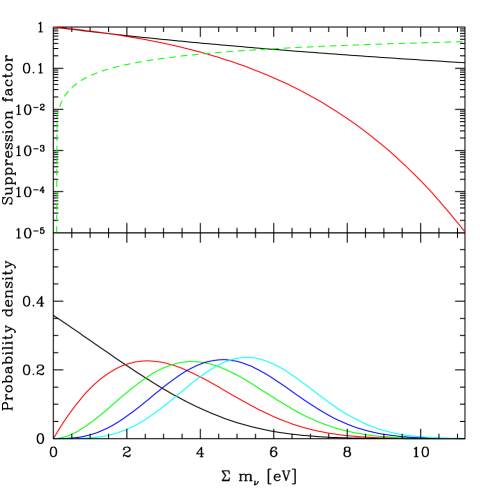
Figure 1: The upper panel shows the factor by which the neutrino fraction $f_{\nu}$ (dashed curve) suppresses the current fluctuation amplitude $\sigma_{M}$ (upper solid curve) and consequently the galaxy number density $n_{G}$ (lower solid curve). The lower panel shows the resulting probability distribution for the neutrino mass sum for priors $m_{\nu}^{n}$ with $n=0$, 1, 2, 3 and 4, peaking from left to right, respectively.

The probability distribution ${\cal P}(m_{\nu})$ is shown in Fig. 1 (bottom) for power law priors

$${\cal P}_{*}(m_{\nu})\propto m_{\nu}^{n},$$ (14)

with $n$ ranging from 0 to 4. For $n\geq 1$, these distributions are peaked at $m_{\nu}\gtrsim 2$ eV, while in the case of a flat prior, ${\cal P}_{*}(m_{\nu})={\rm const}$, the expected values are $m_{\nu}\sim 1$ eV. This is also seen in Fig. 2, where the distribution for a flat prior is shown using a logarithmic scale for $m_{\nu}$.

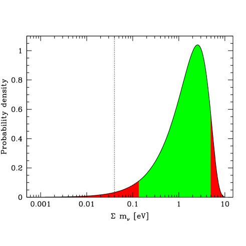
Figure 2: The probability distribution for the neutrino mass sum for flat prior $(n=0)$. The dark/red tails contain 5% probability each. The dotted line shows the lower limit 0.05 eV from atmospheric neutrino oscillations Fukuda99 ; Kearns02 ; Bahcall03 ; King03 .

In this discussion, we have assumed that $f_{\nu}\ll 1$, that is, $m_{\nu}\ll 10$ eV. Very heavy neutrinos (with $m_{\nu}\gg 1$ MeV) would annihilate well before nucleosynthesis and cause no problems with structure formation. If all neutrinos were heavy, neutrons would be stable, leading to an equal number of protons and neutrons. As a result, most of the matter would end up in helium instead of hydrogen. This lack of hydrogen would clearly suppress $n_{obs}(m_{\nu})$ for observers like us who rely on long-lived (hydrogen burning) stars and water-based chemistry. Moreover, heavy neutrinos would not be able to blow off the envelope in supernova explosions. This means that heavy elements formed in stellar interiors would not be dispersed to form planets and observers. The possibility of the electron neutrino being light and one or two others very heavy is allowed anthropically, but it is already ruled out by the neutrino oscillation experiments, which constrain the mass differences to be within $0.05$ eV.

For $m_{\nu}\gg 100$ eV (but $\ll 1$ MeV), keeping all other physical parameters fixed, neutrinos would have sufficiently low thermal velocities to act approximately as cold dark matter, thereby allowing galaxy-size halos to form. However, the baryon fraction in these halos would be strongly diluted, and it is therefore far from clear whether they would be able to cool and form self-gravitating baryonic disks, let alone stars or observers, with an efficiency comparable to that in our observable universe. In other words, the calculation of anthropic constraints on very large neutrino masses becomes essentially equivalent to the calculation of an anthropic upper bound on the dark matter abundance. We will not attempt to address this issue here, but simply assume that the number of observers $n_{obs}(m_{\nu})$ is strongly suppressed for $m_{\nu}\gg 10$ eV.

We have also assumed that there are $N_{\nu}=3$ stable neutrinos. Generalizing our result to $N_{\nu}>3$ is straightforward: as long as the masses are low enough for neutrino infall to be negligible, the galaxy number density depends only on the total neutrino mass density, which for standard neutrino freezeout is proportional to the sum of the neutrino masses. If the neutrinos are unstable on cosmological timescales, they suppress fluctuation growth only before decaying, with their decay radiation redshifting away to gravitationally negligible levels within a few expansion times.

III Prior distribution

Following DV , we shall now discuss possible modifications of the standard particle physics model that could make neutrino masses variable. For early work on how masses of elementary particles can vary randomly in the context of stochastic gauge theories, see Nielsen1 ; Nielsen2 ; Nielsen3 .

Dirac-type neutrino masses can be generated if the Standard Model neutrinos $\nu^{\alpha}$ mix through the Higgs doublet VEV $\Phi$ to some gauge-singlet fermions $\nu_{c}^{\beta}$,

$$g_{\alpha\beta}\Phi{\bar{\nu}}^{\alpha}\nu_{c}^{\beta}.$$ (15)

The couplings $g_{\alpha\beta}$ will generally be variable in string theory inspired models involving antisymmetric form fields $F_{a}$ interacting with branes. (Here, the index $a$ labels different form fields.) $F_{a}$ changes its value by $\Delta F_{a}=q_{a}$ across a brane, where $q_{a}$ is the brane charge. In the low-energy effective theory, the Yukawa couplings $g_{\alpha\beta}$ become functions of the form fields,

$$g_{\alpha\beta}=g_{\alpha\beta}^{(0)}+\sum g_{\alpha\beta}^{a}{F_{a}\over{M_{p}^{2}}}+...,$$ (16)

where the summation is over all form fields, the coefficients $g_{\alpha\beta}^{(0)}$, $g_{\alpha\beta}^{a}$ are assumed to be numbers $\sim 1$, and $M_{p}$ is the effective cutoff scale, which we assume to be the Planck mass.

In such models, closed brane bubbles nucleate and expand during inflation Brown , creating exponentially large regions with different values of the neutrino masses. When $F_{a}$ changes in increments of $q_{a}$, $m_{\nu}$ changes in increments of

$$\Delta m_{\nu}\sim\Phi q_{a}/M_{p}^{2}.$$ (17)

To be able to account for neutrino masses $\lesssim 1$ eV, we have to require that $\Delta m_{\nu}\lesssim 1$ eV, that is,

$$q_{a}\lesssim 10^{-11}M_{p}^{2},$$ (18)

for at least some of the brane charges. Such small values of the charges can be achieved using the mechanisms discussed in Bousso ; DV01 ; Banks ; Feng .

It should be noted that the Higgs potential and the Higgs expectation value $\Phi$ will also generally depend on $F_{a}$. Moreover, each field $F_{a}$ contributes a term $F_{a}^{2}/2$ to the vacuum energy density $\rho_{\Lambda}$, and regions with different values of $F_{a}$ will generally have different values of $\rho_{\Lambda}$. However, in the presence of several form fields with sufficiently small charges, variations of all these parameters are not necessarily correlated, and here we shall assume that there is enough form fields to allow independent variation of the relevant parameters. We can then consider a sub-ensemble of regions with $m_{\nu}$ variable and all other parameters fixed. The probability distribution for $m_{\nu}$ that we calculated in Section II corresponds to such a sub-ensemble.

Let us now turn to the prior distribution ${\cal P}_{*}(m_{\nu})$. The natural range of variation of $F_{a}$ in Eq. (16) is the Planck scale, and the corresponding range of the neutrino masses is $0\leq m_{\nu}^{(i)}\lesssim\Phi$. (Here, the index $i$ labels the three neutrino mass matrix eigenvalues.) Only a small fraction of this range corresponds to values of anthropic interest, $m_{\nu}\lesssim 10$ eV. In this narrow anthropic range, we expect that the probability distribution for $F_{a}$ after inflation is nearly flat GV01 ,

$$d{\cal P}_{*}={\rm const}\cdot dF_{1}dF_{2}...,$$ (19)

and that the the functions $g_{\alpha\beta}(F_{a})$ are well approximated by linear functions. If all three neutrino masses vary independently, this implies that

$$d{\cal P}_{*}={\rm const}\cdot dm_{\nu}^{(e)}dm_{\nu}^{(\mu)}dm_{\nu}^{(\tau)}.$$ (20)

The probability for the combined mass $m_{\nu}=\sum m_{\nu}^{(i)}$ to be between $m_{\nu}$ and $m_{\nu}+dm_{\nu}$ is then proportional to the volume of the triangular slab of thickness $\sim dm_{\nu}$ in the 3-dimensional mass space,

$$d{\cal P}_{*}\propto m_{\nu}^{2}dm_{\nu}.$$ (21)

Alternatively, the neutrino masses can be related to one another, for example, by a spontaneously broken family symmetry. If all three masses are proportional to a single variable mass parameter, then we expect

$$d{\cal P}_{*}\propto dm_{\nu}.$$ (22)

Let us now assess how well the predictions derived from the prior distributions (21) and (22) agree with observations. We first consider the distribution (21), corresponding to independently varying neutrino masses. The most probable value of $m_{\nu}$ for $n=2$ is $m_{\nu}\sim 3$ eV, and we expect both the neutrino masses and mass differences to be $\sim 1$ eV. This expectation, however, is in conflict both with neutrino oscillation experiments suggesting $\Delta m_{\nu}\lesssim 0.05$ eV Fukuda99 ; Kearns02 ; Bahcall03 ; King03 and with astrophysical bounds Spergel03 ; sdsspars which indicate a combined mass $m_{\nu}\lesssim 1$ eV.

For a flat prior distribution (22), the most probable value is $m_{\nu}\sim 1$ eV. If $m_{\nu}$ is close to this value, then the three neutrino masses must be nearly degenerate, with $\Delta m_{\nu}\ll m_{\nu}$. This could be interpreted as a sign of a family symmetry. A 90% confidence level prediction for $m_{\nu}$ based on this distribution can be obtained as outlined in Section II. This gives

$$0.1~{}{\rm eV}<m_{\nu}<5~{}{\rm eV}.$$ (23)

The lower bound in (23) is somewhat stronger than the bound from the neutrino oscillation data Fukuda99 ; Kearns02 ; Bahcall03 ; King03 ($m_{\nu}\mathrel{\hbox to0.0pt{\lower 3.0pt\hbox{$\mathchar 536\relax$}\hss}\raise 2.0pt\hbox{$\mathchar 318\relax$}}0.05~{}{\rm eV}$), while the upper bound is somewhat weaker than the current astrophysical bounds (e.g., Spergel03 ; Hannestad0303076 ; ElgaroyLahav0303089 ; BashinskySeljak03 ; Hannestad0310133 ; sdsspars ). Note that the strength of current astrophysical bounds is limited not by statistical errors but by systematic uncertainties in non-CMB data. For instance, the recently claimed evidence for $m_{\nu}>0$ Allen0306386 may result from underestimated galaxy cluster modeling uncertainties.

We finally mention the possibility that the right-handed neutrinos $\nu_{c}^{\alpha}$ have a large Majorana mass $M_{R}\gg\Phi$. In this case, small neutrino masses can be generated through the see-saw mechanism,

$$m_{\nu}\sim g^{2}\Phi^{2}/M_{R}.$$ (24)

If $M_{R}$ is variable, say, within a range $M_{R}\lesssim M_{p}$, then its most probable values are likely to be $\sim M_{p}$, and the prior distribution will be peaked at very small values of $m_{\nu}\sim 10^{-6}$ eV.

This discussion suggests that the most promising scenario with variable neutrino masses is the one with Dirac-type masses determined by a single variable mass parameter. It yields a flat prior distribution for $m_{\nu}$, Eq. (22), and the prediction (23) at 90% confidence level.

After we submitted the original version of this paper, Jaume Garriga pointed out to us that see-saw-type models can yield cosmologically interesting prior distributions for $m_{\nu}$ if the Majorana mass is restricted to the range $M_{R}<M_{R}^{(max)}\ll M_{p}$. Assuming first that $M_{R}$ is a fixed constant, while $g$ is variable, Eq. (24) yields the distribution

$$d{\cal P}_{prior}\propto dg\propto m^{-1/2}dm.$$ (25)

This would give a somewhat smaller predicted neutrino mass than the distribution (22) that we used in most of our calculations.

The distribution (25) applies up to $m_{max}\sim\Phi^{2}/M_{R}$. In order to have $m_{max}\gtrsim 0.1$ eV, we need $M_{R}\lesssim 10^{13}$ GeV.

If both $M_{R}$ and $g$ are variable, then, assuming a flat prior for $M_{R}$, Eq. (25) still applies, but now $m_{max}\sim\Phi^{2}/M_{R}^{(max)}$, so we need $M_{R}^{(max)}\lesssim 10^{13}$ GeV. An attractive feature of this scenario is that the increment of $m_{\nu}$ in Eq.(17) gets suppressed by an additional factor $\Phi/M_{R}$, and Eq.(18) gets replaced by a much weaker constraint $q_{a}/M_{p}^{2}\lesssim(M_{R}/10^{13}~{}{\rm GeV})^{-1}$.

IV Discussion

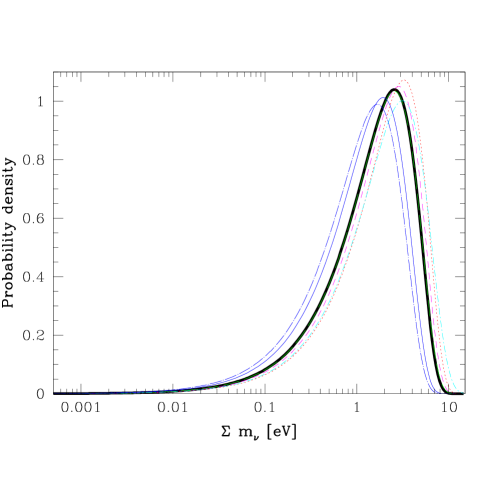
Figure 3: Same as Figure 2, but showing the robustness of the results to changing various assumptions. We have changed the baseline calculation from Figure 2 (heavy black curve) by evaluating the galaxy density in the infinite future $x\to\infty$ (dotted red/grey curve) and at redshift unity, $x=7/3(1+z)^{3}=7/24$ (dot-long-dashed blue/grey curve), decreasing the density threshold to $\delta_{c}=1.5$ (short-dashed magenta/grey curve), lowering the primordial fluctuation amplitude on the galactic scale by 25% (solid blue/grey curve), including the baryon correction as per Eisenstein & Hu (long-dashed green curve) and additionally including the neutrino infall correction as per Eisenstein & Hu (dot-dashed cyan/grey curve).

In conclusion, we have found that the small values of the neutrino masses may be due to anthropic selection. If so, then the most promising model appears to be the one with a flat prior distribution, ${\cal P}_{*}(m_{\nu})={\rm const}$. The range of $m_{\nu}$ predicted in this model, Eq. (23), has interesting implications for both particle physics and cosmology. On the particle physics side, neutrino masses in this range are nearly degenerate, suggesting extensions of the Standard Model involving a spontaneously broken family symmetry. On the cosmological side, a combined neutrino mass of $\gtrsim 1$ eV has a non-negligible effect on galaxy formation. This means that it must be taken into account in precision tests of inflation that measure the shape of the primordial power spectrum by combining microwave background and large-scale structure data.

Let us close by discussing the importance of the assumptions we have made and outlining some open problems for future work. The purpose of this brief paper and the prediction of equation (23) is merely to demonstrate that anthropic selection effects may be able to explain the neutrino masses, and much work needs to be done to place this hypothesis on a firmer footing.

IV.1 Robustness to approximations and measurement errors

To quantify the robustness of our results, Figure 3 shows how the probability distribution for $m_{\nu}$ changes when various assumptions are altered.

First of all, the parameters $A_{\Lambda}$ and $\sigma_{M}(0)$ that we used have non-negligible measurement uncertainties. We see that lowering $\sigma_{M}(0)$ by 25% (by about twice its measurement uncertainty) lowers the $m_{\nu}$-prediction slightly. Changing $A_{\Lambda}$ by within its observational uncertainty has an even weaker effect since, as we saw, it enters only logarithmically. Altering the galactic scale $M$ affects $\sigma_{M}$ and hence the results only weakly, because of the flatness of the dimensionless power spectrum $k^{3}P(k)$ on galactic scales.

Second, our calculations involved various approximations. We used the Press-Schechter approximation with density threshold $\delta_{c}\approx 1.69$ as per Appendix A; lowering this to account for post-virialization infall as discussed in Martel98 is seen to raise the $m_{\nu}$-prediction slightly. Our fluctuation growth treatment of equation (5) is highly accurate in the limit of small mass scales $M$ and low baryon fraction $\Omega_{b}/\Omega_{m}\ll 1$, agreeing with a CMBfast cmbfast numerical calculation to within a few percent. Figure 3 shows that for the observed baryon fraction $\Omega_{b}/\Omega_{m}\approx 0.15$, switching to an exact treatment of baryon effects makes virtually no difference. The cosmic expansion eventually slows neutrinos enough for them to start clustering on galaxy scales, and if this happens before dark energy domination, then it reduces $\gamma$ equation (13). Since a small fraction of the neutrinos will be in the low tail of their velocity distribution, there is a slight infall correction even for the low $m_{\nu}$-range we have considered, and Figure 3 shows that this increases our $m_{\nu}$-prediction slightly. Finally, we have used the cutoff value of $x\approx 7/3$, which amounts to using the reference class of observers in galaxies that have formed by now. Figure 3 shows that if we ask instead what would be observed from a random galaxy among all galaxies that ever form (setting $x=\infty$), then the $m_{\nu}$-prediction increases slightly. Conversely, it also shows that considering only observers in galaxies that formed by redshift unity decreases the $m_{\nu}$-prediction. In conclusion, Figure 3 shows that although many of these assumptions make marginal differences, none of them affect the qualitative conclusions, since they all shift the predicted probability distribution by much less than one standard deviation.

IV.2 Effects of other parameters

The standard models of cosmology and particle physics involve of order 10 and 28 free parameters, respectively. In order to apply anthropic constraints to them, it is crucial to know both which of them can vary, and what the interdependencies or correlations between them are. It is likely that at least some of the cosmological parameters (the baryon-to-photon ratio, say, via baryogenesis) are determined by particle physics parameters in a way that we have yet to understand, and many particle physics parameters may in turn be determined by a smaller number of parameters or vacuum expectation values of some deeper underlying theory. A proper analysis of anthropic predictions should therefore be done in the multi-dimensional space spanned by all fundamental variable parameters.

Such correlations between parameters must ultimately be taken into account not only for computing the theoretical prior ${\cal P}_{*}$ of equation (1), but also when computing the factor $n_{obs}$ in this equation, which incorporates the observational selection effect. The reason is that strong degeneracies are present which can in many cases offset a detrimental change in one parameter by changes in others. For instance, suppressed galaxy formation caused by increased $m_{\nu}$ can to some extent be compensated by decreasing $\rho_{\Lambda}$, by increasing the dark-matter-to-photon ratio or by increasing the CMB fluctuation amplitude $Q$ above the value $\sim 10^{-5}$ that we observe Q ; Aguirre — if any of these three parameters can vary, that is. In the present paper, we have merely considered the simple case where all relevant parameters except $m_{\nu}$ (i.e., the comoving densities of baryons and dark matter, the physical density of dark energy, and the fluctuation amplitude $Q$) are kept fixed at their observed values, with no account for scatter due to variation across an ensemble or from measurement uncertainties. A more detailed study of this issue is given in anthrolambdanu and shows that our present results for $f_{\nu}$ are rather robust to assumptions about $\rho_{\Lambda}$.

This is closely related to the issue of how much information one wishes to include in the factor $n_{obs}$ in equation (1) Bostrom ; Aguirre . One extreme is including only the existence of observers, the other extreme is including all available knowledge (even, say, experimental constraints on $m_{\nu}$). As one includes more such information, the anthropic factor becomes progressively less important, and the calculation acquires the flavor of a prediction rather than an explanation. In the context of a multiparameter analysis, the question is whether to use the measured values of other parameters (in our case non-neutrino parameters) or marginalize over them. Our fixing non-neutrino parameters at their observed values is therefore equivalent to factoring in the information from the measurements of these parameters.

Arguably the most interesting outstanding question is whether the fundamental equations that govern our Universe do or do not allow physical quantities such as the neutrino masses to vary from place to place. Calculations of anthropic selection effects may prove useful for shedding light on this. In any case, for quantities that do vary, the inclusion of anthropic selection effects such as the one we have evaluated in this paper is clearly not optional when calculating what the theory predicts that we should observe.

We thank Anthony Aguirre, Gia Dvali, Jaume Garriga, Martin Rees and Douglas Scott for helpful comments. MT was supported by NSF grants AST-0071213 & AST-0134999, NASA grant NAG5-11099, by a David and Lucile Packard Foundation fellowship and a Cottrell Scholarship from Research Corporation. AV was supported in part by the National Science Foundation and the John Templeton Foundation.

Appendix A Growth of linear perturbations

In this Appendix, we derive and test the approximation given by equation (5) for how small-scale matter fluctuations grow in the presence of radiation, cold dark matter and neutrinos. There are two reasons why this simple approximation complements an exact “black box” calculation with CMBfast cmbfast or a nearly exact approximation with the Eisenstein & Hu fitting software EisensteinHu99 . First, for a qualitative argument like the one we make in this paper, it is desirable to have a simple intuitive understanding of the underlying physics that includes only those complications that really matter for the argument. Second, neither CMBfast nor the Eisenstein & Hu package were designed to be valid for extreme cosmological parameters such as those corresponding to the infinite future, and indeed break down in this limit.

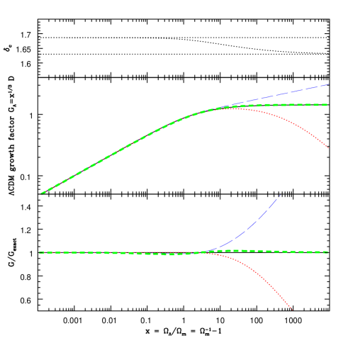
Figure 4: The LCDM growth function $G_{\Lambda}$ is shown as a function of cosmic time, first growing as the scale factor $a\propto x^{1/3}$, then asymptoting to $1.44$ as dark energy halts the fluctuation growth at $x\mathrel{\hbox to0.0pt{\lower 3.0pt\hbox{$\mathchar 536\relax$}\hss}\raise 2.0pt\hbox{$\mathchar 318\relax$}}1$. The middle panel shows the exact result of equation (26) (solid curve), our approximation given by equation (7) (green thick dashed curve), the Carroll, Press & Turner approximation Carroll92 (red dotted curve) and the power law approximation $G_{\Lambda}=\Omega_{\rm m}^{0.21}$ openreion (blue long-dashed curve). In the bottom panel, the various approximations have been divided by the exact result, showing that equation (5) is accurate to better than 1.5% for all $x$. The top panel shows the collapse density threshold $\delta_{c}(x)$ dropping from $1.6865$ early on to $1.62978$ in the infinite future.

A.1 The $\Lambda$CDM case

For a flat Universe with only pressureless matter (dark and baryonic) and a cosmological constant, the growth of density fluctuations is given by $\delta\propto G_{\Lambda}(x)$, where Heath77 ; Martel98

$$G_{\Lambda}(x)={5\over 6}\sqrt{1+{1\over x}}\int_{0}^{x}{dy\over y^{1/6}(1+y)^{3/2}}.$$ (26)

We find that our $G_{\Lambda}(x)$ fit defined by equation (7) is accurate to better than 1.5% for all $x$ and becomes exact both in the limits $x\to 0$ (when $G_{\Lambda}\to x^{1/3}$) and $x\to\infty$ (when $G_{\Lambda}\to G_{\infty}$). Figure 4 shows that this approximation greatly improves on the standard Carroll, Press & Turner Carroll92 and power law fits for our present purposes, since these were designed to be accurate only in the past and present and have the wrong limiting behavior in the future as $x\to\infty$, $\Omega_{\rm m}\to 0$ and $\Omega_{\Lambda}\to 1$. For flat models, we have $\Omega_{\rm m}=1/(1+x)$, $\Omega_{\Lambda}=x/(1+x)$ and $x=(\Omega_{\rm m}^{-1}-1)^{-1}$, so in terms of the standard linear growth factor $D\equiv G_{\Lambda}/x^{1/3}$, the three approximations shown in Figure 4 are

$$D\approx\left[1+\left({1-\Omega_{\rm m}\over\Omega_{\rm m}G_{\infty}^{3}}\right)^{\gamma}\right]^{-1/3\gamma},$$ (27)

$$D \approx {5\over 2}\Omega_{\rm m}\left[\Omega_{\rm m}^{4/7}-\Omega_{\Lambda}+\left(1+{\Omega_{\rm m}\over 2}\right)\left(1+{\Omega_{\Lambda}\over 70}\right)\right]^{-1}$$ (28)

$$= {350\Omega_{\rm m}\over 140\Omega_{\rm m}^{4/7}+(209-\Omega_{\rm m})\Omega_{\rm m}+2}$$

and

$$D\approx\Omega_{\rm m}^{-0.21},$$ (29)

respectively.

A.2 Including radiation

Early on, dark energy was negligible but radiation was gravitationally important, causing density fluctuations to grow as $\delta\propto G_{\gamma}(x)$, where PeeblesOpus

$$G_{\gamma}(x)=1+{3\over 2}\left({x\over x_{\rm eq}}\right)^{1/3}.$$ (30)

Since both $G_{\gamma}(x)$ and $G_{\Lambda}(x)$ accurately describe the growth during the matter-dominated epoch $x_{\rm eq}\ll x\ll 1$, with $G_{\gamma}\propto G_{\Lambda}\propto x^{1/3}$ during this period, we can combine them to obtain the approximation

$$G(x)\approx 1+{3\over 2}A_{\Lambda}G_{\Lambda}(x),$$ (31)

which is accurate for all $x$. Here the constant $A_{\Lambda}$ is defined by equation (10). In essence, fluctuations grow as $\delta\propto a\propto x^{1/3}$ between matter domination ($x=x_{\rm eq}$) and dark energy domination ($x=1$), giving a net growth of $A_{\Lambda}=x_{\rm eq}^{-1/3}$. Equation (31) shows that they grow by an extra factor of 1.5 by starting slightly before matter domination and by an extra factor $G_{\Lambda}(\infty)\approx 1.44$ by continuing to grow slightly after dark energy domination.

A.3 Including neutrinos

As shown by Bond80 , the result $\delta\propto a$ is generalized to $\delta\propto a^{p}$ when a fraction of the matter is clustering inert and remains spatially uniform. The new exponent $p<1$ is given by equation (12) where, in the case that we are focusing on here, the inert fraction is the neutrino fraction $f_{\nu}$. This motivates our approximation in equation (5), which simply generalizes equation (31) by introducing the neutrino-dependent exponent $p(f_{\nu})$.

We have tested this approximation by comparing equation (5) with exact results using the CMBfast software cmbfast and the semianalytic approximation of Eisenstein & Hu EisensteinHu99 , finding excellent agreement (to within a few percent) with both in the small-scale limit for $x\sim 1$ and negligible baryon fraction. In the distant future limit $x\to\infty$, both CMBfast and the Eisenstein & Hu software break down, since they were not designed to be accurate for such unusual parameter values ($\Omega_{\Lambda}=1$, etc.). For the parameter ranges of interest to us, there are small corrections for the effects of both baryons and neutrino infall, which we quantified in Figure 3 in the discussion section.

A.4 The collapse density threshold $\delta_{c}$

In the top panel of Figure 4, we have numerically computed the collapse density threshold $\delta_{c}$ as a function of cosmic time $x$, defined as the linear perturbation theory overdensity that a top hat fluctuation would have had at the time when it collapses. We see that it varies only very weakly with time (note the expanded vertical scale in the figure), dropping from the familiar cold dark matter value $\delta_{c}(0)=(3/20)(12\pi)^{2/3}\approx 1.68647$ early on to the limit $\delta_{c}(\infty)=(9/5)2^{-2/3}G_{\infty}\approx 1.62978$ Weinberg87 in the infinite future. This calculation neglects the effect of neutrinos. Since their effect is to contribute a gravitationally inert component just as dark energy, we will ignore their effect on $\delta_{c}(x)$, assuming that they merely cause a slight horizontal stretching of the curve (which is seen to be almost constant anyway).

References

- (1) P.C.W. Davies and S. Unwin, Proc. Roy. Soc. 377, 147 (1981).
- (2) J. D. Barrow and F. J. Tipler, The Anthropic Cosmological Principle (Oxford, Clarendon Press, 1986).
- (3) A.D. Linde, in 300 Years of Gravitation, ed. by S.W. Hawking and W. Israel, Cambridge University Press, Cambridge (1987).
- (4) S. Weinberg, Phys. Rev. Lett. 59, 2607 (1987).
- (5) A. Vilenkin, Phys. Rev. Lett. 74, 846 (1995).
- (6) G. Efstathiou, MNRAS 274, L73 (1995).
- (7) H. Martel, P. R. Shapiro, and S. Weinberg, ApJ 492, 29 (1998).
- (8) For a recent discussion and references see J. Garriga and A. Vilenkin, Phys. Rev. D67, 043503 (2003).
- (9) A. Vilenkin, Phys. Rev. D27, 2848 (1983).
- (10) A. D. Linde, Phys. Lett. 175B, 395 (1986).
- (11) For a review see A. D. Linde, Particle Physics and Inflationary Cosmology (Chur, Switzerland, Harwood, 1990).
- (12) R. Bousso and J. Polchinski, JHEP 0006:006 (2000).
- (13) T. Banks, M. Dine and L. Motl, JHEP 0101:031 (2001).
- (14) J.F. Donoghue, Int. J. Mod. Phys. A16S1C, 902 (2001).
- (15) L. Susskind, hep-th/0302219 (2003).
- (16) B. Carr and M. J. Rees, Nature 278, 605 (1979).
- (17) M. J. Rees, Physica Scripta 21, 614 (1979).
- (18) A. D. Linde, Phys. Lett. B 201, 437 (1988).
- (19) A. D. Linde and M. I. Zelnikov, Phys. Lett. B 215, 59 (1988).
- (20) A. D. Linde, Phys. Lett. B 351, 99 (1995).
- (21) J. García-Bellido and A. D. Linde, Phys. Rev. D 251, 429 (1995).
- (22) A. Vilenkin, in Cosmological constant and the evolution of the universe, ed by K. Sato, T. Suginohara and N. Sugiyama (Universal Academy Press, Tokyo, 1996); gr-qc/9512031.
- (23) A. Vilenkin and S. Winitzki, Phys. Rev. D 55, 548 (1997).
- (24) M. Tegmark and M. J. Rees, ApJ 499, 526 (1998).
- (25) M. Tegmark, Class. Quant. Grav. 14, L69 (1997).
- (26) M. Tegmark, Ann. Phys. 270, 1 (1998).
- (27) B. Agrawal, S.M. Barr, J.F. Donoghue and D. Seckel, Phys. Rev. Lett. 80, 1822 (1998); Phys. Rev. D57, 5480 (1998).
- (28) J.F. Donoghue, Phys. Rev. D57, 5499 (1998).
- (29) J. Garriga, T. Tanaka and A. Vilenkin, Phys. Rev. D60, 023501 (1999).
- (30) J. Garriga, M. Livio and A. Vilenkin, Phys. Rev. D61, 023503 (2000).
- (31) C. J. Hogan, Rev. Mod. Phys. 72, 1149 (2000).
- (32) A. Aguirre, PRD 64, 083508 (2001).
- (33) M. Tegmark, astro-ph/0302131 (2003).
- (34) W. H. Press and P. Schechter, ApJ 187, 425 (1974).
- (35) J. R. Bond, G. Efstathiou, and J. Silk,, PRL 45, 1980 (1980).
- (36) D. N. Spergel et al., ApJS 148, 175 (2003).
- (37) M. Tegmark et al., PRD 69, 103501 (2004).
- (38) G. Hinshaw et al., ApJS 148, 135 (2003).
- (39) M. Tegmark et al., ApJ 606, 702 (2004).
- (40) V.A. Rubakov and M.E. Shaposhnikov, Mod. Phys. Lett. A4, 107 (1989).
- (41) Y. Fukuda et al., Phys. Rev. Lett. 82, 1810 (1999).
- (42) E. T. Kearns, hep-ex/0210019 (2002).
- (43) J. N. Bahcall, JHEP 0311, 004 (2003).
- (44) S. King, Rept. Prog. Phys. 67, 107 (2004).
- (45) G. Dvali and A. Vilenkin, unpublished.
- (46) H. B. Nielsen and C. D. Froggatt, Nucl. Phys B 147, 277 (197?).
- (47) H. B. Nielsen and C. D. Froggatt, Nucl. Phys B 164, 114 (1980).
- (48) C. D. Froggatt and H. B. Nielsen, Origin of Symmetries (Singapore, World Scientific, 1991).
- (49) J.D. Brown and C. Teitelboim, Nucl. Phys. 279, 787 (1988).
- (50) G. Dvali and A. Vilenkin, Phys. Rev. D64, 063509 (2001).
- (51) J.L. Feng, J. March-Russell, S. Sethi and F. Wilczek, Nucl. Phys. B602, 307 (2001).
- (52) J. Garriga and A. Vilenkin, Phys. Rev. D64, 023517 (2001).
- (53) S. Hannestad, JCAP 05, 004 (2003).
- (54) O. Elgaroy and O. Lahav, JCAP 0304, 004 (2003).
- (55) S. Bashinsky and Seljak U, PRD 69, 083002 (2004).
- (56) S. Hannestad, astro-ph/0310133 (2003).
- (57) S. W. Allen, R. W. Schmidt, and S. L. Bridle, MNRAS 346, 593 (2003).
- (58) U. Seljak, and M. Zaldarriaga, ApJ 469, 437 (1996).
- (59) L. Pogosian, A. Vilenkin, and M. Tegmark, JCAP 407, 5 (2004).
- (60) N. Boströ m, Anthropic Bias: Observation Selection Effects in Science and Philosophy (New York, Routledge, 2002).
- (61) D. J. Eisenstein and W. Hu, ApJ 511, 5 (1999).
- (62) S. M. Carroll, W. H. Press, and E. L. Turner, ARA&A 30, 499 (1992).
- (63) M. Tegmark and J. Silk, ApJ 441, 458 (1995).
- (64) D. J. Heath, MNRAS 179, 351 (1977).
- (65) P. J. E. Peebles,Principles of Physical Cosmology, Princeton University Press, Princeton, New Jersey (1993).
- (66) C. P. Ma, ApJ 471, 13 (1996).