The Composition of the Interstellar Medium towards the Lockman Hole

The Lockman Hole is well known as the region with the lowest neutral atomic hydrogen column density on the entire sky. We present an analysis of the soft X-ray background radiation towards the Lockman Hole using ROSAT all-sky survey data. This data is correlated with the Leiden/Dwingeloo survey (Galactic H i 21 cm-line emission) in order to model the soft X-ray background by using radiative transfer calculations for four ROSAT energy bands simultaneously. It turns out, that an important gas fraction, ranging between 20–50%, of the X-ray absorbing material is not entirely traced by the H i but is in the form of ionized hydrogen. Far-ultraviolet absorption line measurements by FUSE are consistent with this finding and support an ionized hydrogen component towards the Lockman Hole.

1 Introduction

In this paper we focus on the Galactic plasma emission with emphasis on the coronal gas in the Milky Way halo. We concentrate our study on the Lockman Hole region on the northern high Galactic latitude sky. The Lockman Hole (e.g. Lockman et al. (1986), Jahoda et al. (1990)) is the sky region with the absolute lowest H i column density ($N_{{H\textsc{i}}}\approx 4.5\cdot 10^{19}\,{\rm cm}^{-2}$). Therefore, it is considered to be the most transparent window to the distant Universe. To test this assumption, we investigate the photoelectric absorption of X-rays by the interstellar medium (ISM).

Towards this aim, we performed a correlation analysis of the ROSAT all-sky survey data with the Leiden/Dwingeloo H i 21 cm-line survey. Both surveys are the state-of-the-art data bases for such an approach. In the soft X-ray energy regime (E $<$ 1 keV) the mean free path length of the X-ray photons are only a few tens of parsec at maximum, assuming a density of $n\simeq 1\,{\rm cm}^{-3}$ (McCammon & Sanders 1990). The exact knowledge of the amount of photoelectric absorbing material is essential to evaluate the soft X-ray radiative transfer through the Galactic ISM. Previous investigations of the Lockman Hole area (Snowden et al. 1994a) showed that diffuse soft X-ray emission originates beyond some H i gas clouds on the line of sight. They concluded that in general the 1/4 keV X-ray emission appears to be anti-correlated with the $N_{{H\textsc{i}}}$. In detail, significant deviations between the localization of individual H i clouds and the X-ray intensity minima are suggested. Moreover, Snowden et al. (1994a) proposed that the X-ray emitting halo gas located beyond the Draco cloud (Snowden et al. 1991) and the one observed towards the Lockman Hole are different in temperature $T$ and emission measure $n_{\rm e}^{2}$ indicating a different origin of both plasmas. This supports the picture of a patchy Milky Way halo gas.

In this paper, we analyze a much larger portion – enclosing the Lockman Hole – of the northern high Galactic latitude sky. We use the ROSAT all-sky survey data of four energy bands, sampling the soft energy regime: 0.25 keV $\leq E\leq$ 0.82 keV. The Leiden/Dwingeloo H i survey data serves as a tracer for the photoelectric absorption, evaluated by the H i column density along the lines of sight. We utilize the velocity information inherent to the H i line spectra to unravel spatially the composition of the ISM towards the Lockman Hole. In particular, we focus on the role of the Warm Neutral Medium (WNM) and the intermediate-velocity cloud gas (IVC) towards this position on the sky.

The paper is organized as follows: Section 2 presents the X-ray and H i data. Section 3 outlines our approach to correlate both data sets, summarizes the best fit parameters for the temperatures, intensities and absorbing column densities. Section 4 describes the far-ultraviolet absorption line analysis of the Lockman Hole. In Section 5 we present our conclusions.

2 The Data

2.1 H i Data

The Leiden/Dwingeloo survey of Galactic neutral hydrogen (Hartmann & Burton 1997) covers the entire sky north of $\delta=-30^{\circ}$ with a true-angle spacing of 0$\aas@@fstack{\circ}$5 in both l and b. The spectrometer used has 1024 channels and a velocity resolution of 1.03 km s^-1 which leads to a LSR velocity coverage of -450 km s^-1 to +400 km s^-1. Hence, most high-velocity cloud (HVC) emission is encompassed by this velocity interval. The rms-noise of the measured brightness-temperature amounts to $\Delta T_{\rm B}=0.07$ K. Moreover, the spectra are corrected for the influence of stray radiation (Kalberla et al. 1980; Hartmann et al. 1996), which is of greatest concern in galactic H i-surveys.

We extracted the sky region bordered by $b=12^{\circ}$…$75^{\circ}$ and $l=99^{\circ}$…$166^{\circ}$ including the Lockman Hole. The lowest H i column density region (Lockman et al. 1986, ($N_{{H\textsc{i}}}\approx 4.5\cdot 10^{19}\,{\rm cm}^{-2}$)) is localized at $(l,b)=(150^{\circ},53^{\circ})$. According to the large stretch in Galactic latitude, the contrast between the highest column density region at low Galactic latitude and the Lockman Hole is about a factor of 25 (equivalent $\simeq$ 14 dB). This high column density contrast gives us the opportunity to disentangle the contribution of the different diffuse X-ray emission components, by focussing on regions where each individual X-ray emission component is observable with high significance. The H i data are binned into velocity integrated maps which are projected on the ROSAT grid for a pixel-by-pixel correlation. This is described in Sect. 3.3. The pixel size is set to 48′, about twice the ROSAT all-sky survey data analyzed here and about $\sqrt{2}$ of the Leiden/Dwingeloo beam size.

2.2 X-ray Data

The X-ray data of the Lockman area were extracted from the ROSAT all-sky survey (RASS) (Snowden et al. 1995, 1997). The data used have an angular resolution of 24′. We investigate four ROSAT energy bands: the R1-band ($E\simeq 0.25$ keV), the R2-band ($E\simeq 0.31$ keV), the C-band ($E\simeq 0.28$ keV), and the M-band ($E\simeq 0.82$ keV) (Snowden et al. 1994b). The data are corrected for scattered solar X-rays (Snowden & Freyberg 1993), particle background (Plucinsky et al. 1993), as well as long–term X-ray enhancements (Snowden et al. 1995). X-ray point sources were removed down to a minimum count rate of 0.02 cts s^-1 (Snowden et al. 1997). The statistical significance of the X-ray data were evaluated by the ROSAT uncertainty maps which only account for the number of photon events: they do not include any systematic uncertainties produced by any non-cosmic X-ray events.

3 Method

3.1 Radiative transfer equation for the ISM

3.1.1 The effective photoelectric absorption

In the soft X-ray energy regime, the photoelectric absorption is the dominant process of X-ray attenuation. According to Morrison & McCammon (1983), the photoelectric absorption cross section is a strong function of energy ($\sigma\propto E^{-\frac{8}{3}}$) and amounts to some $\sigma\simeq 10^{-20}\,{\rm cm}^{2}$ (according to ROSAT C-band) for an ISM of solar metalicity and $n\simeq 1\,\mathrm{cm^{-3}}$. Both findings highlight two important facts: a) the lower the X-ray photon energy the higher the probability of photoelectric absorption and b) all lines of sight through the Galactic ISM are optically thick for soft X-ray emission – except for the Lockman Hole. As pointed out in Sect. 2.2, we analyze the X-ray intensity distribution of broad energy bands. According to this approach, it is necessary to evaluate the X-ray band–averaged photoelectric absorption cross section, the so-called effective photoelectric absorption cross section:

$$\sigma(N_{{H\textsc{i}}})=-\frac{1}{N_{{H\textsc{i}}}}\ln\left\{\frac{\int S(E)\cdot T(E)\cdot{\rm e}^{-\sigma^{\prime}(E)\cdot N_{{H\textsc{i}}}}{\rm\cdot dE}}{\int S(E)\cdot{\rm e}^{-\sigma^{\prime}(E)\cdot N_{{H\textsc{i}}}}{\rm\cdot dE}}\right\}$$ (1)

Here $S(E)$ denotes the spectrum of the X-ray source, $T(E)$ the telescope and detector response function, $\sigma^{\prime}(E)$ the Morrison & McCammon (1983) photoelectric cross section, $N_{{H\textsc{i}}}$ the observed H i column density (for details see Kerp et al. 1999). Using this effective photoelectric absorption cross section $\sigma(N_{{H\textsc{i}}})$ yields an inherent ambiguity: without an educated guess of $S(E)$ it is not possible to determine $\sigma(N_{{H\textsc{i}}})$. In consequence, we have to compare the observational data with a variety of different spectral models to overcome this ambiguity.

3.1.2 Galactic $N_{{H\textsc{i}}}$

The distribution of the general ISM of the Milky Way is traced by the Galactic H i 21 cm-line emission. It is thought that H i – as the most abundant element in space – traces the distribution of the metals quantitatively.

Early H i surveys already revealed that H i clouds exist next to the rotating Galactic disk, which cannot be modeled within the framework of co-rotating ISM. Based on these early findings, today we distinguish between low-, intermediate- and high-velocity clouds (Dickey & Lockman 1990). In the following we will show, that low- and intermediate-velocity clouds can be identified as soft X-ray shadows against the distant diffuse X-ray background emission (e.g. Snowden et al. (2000)). To differentiate between these different constituents of the ISM we bin the data into velocity integrated maps covering $|v_{\mathrm{LSR}}|<25\,{\rm km\,s^{-1}}$, $|v_{\mathrm{LSR}}|<75\,{\rm km\,s^{-1}}$ and $|v_{\mathrm{LSR}}|<100\,{\rm km\,s^{-1}}$. We show that the $|v_{\mathrm{LSR}}|<75\,{\rm km\,s^{-1}}$ already covers H i gas belonging to the M81/M82 group of galaxies. This intra-group H i gas allows a critical test of our X-ray vs. H i correlation analysis because it is accidentally included in the radiative transfer equation as an absorber within the $|v_{\mathrm{LSR}}|<75\,{\rm km\,s^{-1}}$ map of the Milky Way halo.

3.2 The individual X-ray source terms

3.2.1 The Local Hot Bubble

Early sounding rocket experiments as well as the Wisconsin X-ray sky survey established the existence of hot X-ray emitting plasma within the local environment of the Sun. This coronal gas fills the irregularly shaped local void of matter (McCammon & Sanders 1990) – frequently called the Local Hot Bubble (LHB). Therefore, the X-ray intensity of the Local Hot Bubble varies appreciable across the entire sky: $I_{\rm LHB}=(2.5\dots 8.2)\cdot 10^{-4}\,{\rm cts\,s^{-1}\,arcmin^{-2}}$ (Snowden et al. 1998). $I_{\rm LHB}$ is the first term in our radiative transport equation (see Eqn. 2). Considering the results of Sfeir et al. (1999) we know that only a few local clouds are intermixed with the hot X-ray emitting plasma of the Local Hot Bubble (e.g. Kerp et al. 1993). Because of this finding, we assume that $I_{\rm LHB}$ is not absorbed by any intervening gas along the line of sight.

3.2.2 The Milky Way halo

The existence of hot coronal gas within the Milky Way halo was one of the major discoveries of the ROSAT mission. Moreover, it was found that the X-ray emission from the LHB has a superposed diffuse component (Snowden et al. 1991; Herbstmeier et al. 1995; Kerp et al. 1996; Pietz et al. 1998) in excess to the contribution of the extragalactic background radiation. It is beyond any doubt that diffuse X-ray emission originates within the Milky Way halo, but it is a matter of debate as to how many thermal plasma components are localized within the Galactic halo (Kuntz & Snowden 2000). Their corresponding individual temperatures and emission measures are also a matter of debate. Here we follow the approach of a hot single halo component which will turn out to be sufficient. We vary the temperature of the Galactic halo plasma and search for a best fit temperature simultaneously consistent with all four ROSAT energy band data. The Milky Way halo is represented as $I_{\rm HALO}$ in the radiative transfer equation (see Eqn. 2). This diffuse X-ray emission component is absorbed by the Galactic ISM along the line of sight. Following the latest results on the scale height of the highly ionized species (Savage et al. 1997, 2003) and prior H i vs. X-ray correlation analysis (Pietz et al. 1998), the scale height of the Milky Way halo plasma is about 4 kpc (Kalberla & Kerp 1998). We can safely assume that all ISM components with a lower scale height, the Warm Neutral Medium (WNM), the Warm Ionized Medium (WIM) and the Cold Neutral Medium (CNM) are in front of this diffuse X-ray emission. This amount of absorbing material has to be evaluated in order to calculate the strength of the photoelectric absorption. We account for the different characteristic scale heights of the neutral species by using the velocity integrated maps defined in Sect. 3.1.2.

3.2.3 The extragalactic component

The extragalactic X-ray background is composed of superposed emission of point sources, in particular of AGNs (e.g. Tozzi et al. 2001). Its spectrum can be approximated by a power law ($E^{-\Gamma}$). We assume an average spectral index of $\Gamma=1.5$ according to Hasinger et al. (2001). Its ROSAT C-band intensity was determined by Barber et al. (1996); they derived $I_{\rm EXTRA}=228\cdot 10^{-6}\,{\rm cts\,s^{-1}\,arcmin^{-2}}$ with an uncertainty of $90\cdot 10^{-6}\,{\rm cts\,s^{-1}\,arcmin^{-2}}$. Throughout the fit procedure (see Sect. 3.3) we will fix $I_{\rm EXTRA}$ to both values normalized to the ROSAT C-band and their corresponding values in the other ROSAT energy bands respectively. We assume that all neutral interstellar matter along the line of sight measured in the Leiden/Dwingeloo H i survey ($N_{{H\textsc{i}},\rm e}$) is in front of the extragalactic sources. Also this amount of photoelectric absorbing material is constant in the evaluation of the soft X-ray radiative transfer calculations.

This leads to the radiative transfer equation for soft X-rays introduced by Kerp et al. (1999):

$$I=I_{\rm LHB}+I_{\rm HALO}\cdot{\rm e}^{-\sigma_{\mathrm{h}}\cdot N_{{H\textsc{i}},{\rm h}}}+I_{\rm EXTRA}\cdot{\rm e}^{-\sigma_{\mathrm{e}}\cdot N_{{H\textsc{i}},{\rm e}}}.$$ (2)

Here, $\sigma_{\rm h}$ denotes the effective photoelectric absorption cross section of the Galactic halo, while $\sigma_{\mathrm{e}}$ represents that for the extragalactic background. While we can safely assume that all H i observed towards a distant AGN is enclosed within the velocity range $-450\,{\rm km\,s^{-1}}<\,v_{\mathrm{LSR}}\,<450\,{\rm km\,s^{-1}}$, we have to question this assumption with respect to the Milky Way. Here we have to identify the best fit velocity range by comparing the H i and the diffuse X-ray data quantitatively. To differentiate between both absorbing column densities we use $N_{{H\textsc{i}},{\rm e}}$ and $N_{{H\textsc{i}},{\rm h}}$ from here on. Equation 2 has four free parameters ($I_{\rm LHB},I_{\rm HALO},T_{\rm LHB},T_{\rm HALO}$) and two fixed parameters ($I_{\rm EXTRA},\Gamma$). The temperatures of the LHB ($T_{\rm LHB}$) and of the Galactic halo ($T_{\rm HALO}$) are connected to Eq. 2 by the source term $S(E)$ in Eq. 1. $N_{{H\textsc{i}},{\rm e}}$ and $N_{{H\textsc{i}},{\rm h}}$ are fixed parameters as well because by optimizing the free parameters both $N_{{H\textsc{i}}}$ values are fixed. To determine the four free parameters, we use the information of the ROSAT R1-, R2-, C- and M-Band in simultaneous fit procedures of X-ray energy band ratios and intensities vs. $N_{{H\textsc{i}},{\rm h}}$.

3.3 Modeling

In order to evaluate the radiative transport equation (Eq. 2) for all ROSAT energy bands and band ratios simultaneously, we developed a two-step fit procedure. The first step (one dimensional approach) gives us the opportunity to estimate the start-values for the fit parameters. The second step (two dimensional approach) is used to derive the spatial distribution of the X-ray intensities correctly. Moreover, we can optimize the fit parameters within the framework of the two dimensional fit procedure.

3.3.1 The one dimensional approach

The radiative transport equation (see Eq. 2) gives us the possibility to derive fit parameters, namely the intensities of the two free emission components. In practice we calculate so–called scatter diagrams (see Fig. 1 for the C-band scatter diagram) for the ROSAT C- and M-band and the energy band ratios R1/R2 and C/M as functions of $N_{H\textsc{i}}$. The energy band ratios are a sensitive measure for the temperature of both X-ray emitting plasmas.

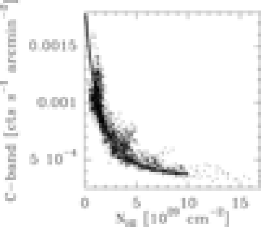
Figure 1: Scatter plot for the ROSAT C-band. At high column densities ($>5\cdot 10^{20}$ cm^-2) the X-ray intensity shows an asymptotic behavior. This represents only the foreground emission of the LHB. The solid line shows the best fit model which satisfies all ROSAT energy bands and band ratios simultanously (see Fig. 2, 3, 4 as well). Other models (i.e. with varying halo- and/or LHB-temperatures) are not distinguishable from each other.

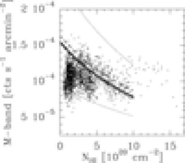
Figure 2: Scatter plot for the ROSAT M-band. The dotted lines correspond to models where the halo plasma temperature is $10^{6.3}$ K (upper curve) and $10^{6.1}$ K (lower curve). The dashed lines correspond to models where the LHB temperature is $10^{5.9}$ K (upper curve) and $10^{6.1}$ K (lower curve). As in Fig. 1 the solid line represents the best fit model.

The first free parameter value we derive is the C-band intensity of the Local Hot Bubble ($I_{\rm LHB}$). The data points in the C-band scatter diagram (Fig. 1) show an asymptotic behavior at high column densities ($>5\cdot 10^{20}\,{\rm cm^{-2}}$). Here we observe only the X-ray foreground emission because the entire background emission of $I_{\mathrm{HALO}}$ and $I_{\mathrm{EXTRA}}$ is absorbed by the high column density in front of both components; therefore, the first estimate is $I_{\rm LHB}=450\cdot 10^{-6}\,{\rm cts\,s^{-1}\,arcmin^{-2}}$ which is consistent with the values given by Snowden et al. (1998).

The $I_{\rm HALO}$ is determined at the low column density part of the C-band and full M-band scatter diagram. In the ROSAT C-band we observe the superposed emission of $I_{\rm LHB}$ and $I_{\rm HALO}$ while in the ROSAT M-band (see Fig. 2) we have to include the diffuse X-ray emission attributed to the extragalactic background.

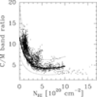
Figure 3: ROSAT C/M-band ratio vs. $N_{{H\textsc{i}}}$. The dotted lines correspond to models where the halo plasma temperature is $10^{6.3}$ K (upper curve) and $10^{6.1}$ K (lower curve). As in Fig. 1 the solid line represents the best fit model. Note, that the dashed lines, representing the variation of $T_{\rm LHB}$ in Fig. 4, are not suitable to evaluate $T_{\rm LHB}$ in the C/M-band ratio.

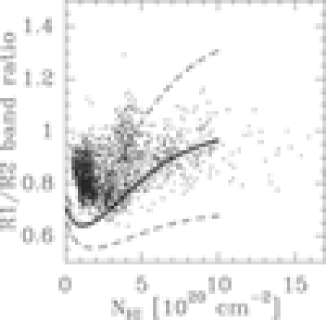
Figure 4: ROSAT R1/R2-band ratio vs. $N_{{H\textsc{i}}}$. The dashed lines correspond to models where the LHB temperature is $10^{5.9}$ K (upper curve) and $10^{6.1}$ K (lower curve). As in Fig. 1 the solid line represents the best fit model. Note, that the dotted lines, representing the variation of $T_{\rm HALO}$ in Fig. 3, are not sensitive to evaluate $T_{\rm HALO}$ in the C/M-band ratio.

Considering only the C-band scatter diagram (Fig. 1), an ambiguity concerning the plasma temperatures remains. Variations of the plasma temperature $T_{\mathrm{HALO}}$ yield insignificant variations in the fitted curves. To constrain $T_{\mathrm{LHB}}$ and $T_{\mathrm{HALO}}$ we plot the R1/R2 and C/B band ratio versus $N_{\mathrm{HI,h}}$ (see Fig. 3 & 4). Regarding these, we see large variations in the C/M Band ratio vs. $N_{\mathrm{HI,h}}$ plot, when we vary the halo plasma temperature in the same way as for the C-band scatter diagram (see Fig. 1). Variations of $T_{\mathrm{LHB}}$ cause significant variations in the R1/R2 band ratio vs. $N_{\mathrm{HI,h}}$ (Fig. 4). An immediate impact on the energy band ratios vs. $N_{\mathrm{HI,h}}$ is seen if we vary $I_{\rm HALO}$ and $I_{\rm LHB}$ individually. Because a variation of only one free parameter has an immediate effect, all four scatter diagrams, we have a sensitive tool to find a consistent solution for all four parameters simultaneously. To illustrate this proposal we plot a set of temperature models for $T_{\mathrm{HALO}}$ in each of the four scatter diagrams while leaving the other parameters $I_{\mathrm{LHB}}$, $I_{\mathrm{HALO}}$ and $T_{\mathrm{LHB}}$ fixed to the best fit parameters given in Sec. 3.4.2. Since the C-band and R1/R2 band ratio scatter diagrams are not sensitive to temperature variations of the parameter $T_{\mathrm{HALO}}$ the M-band and C/M band ratio scatter diagrams show up with significant deviations from the best fit situation marked by the solid line.

In Fig. 4 we demonstrate the variation of the $T_{\mathrm{LHB}}$ on the R1/R2 band ratio scatter diagram. While the C- and M-band scatter diagrams as well as the C/M ratio scatter diagram are not sensitive measures for $T_{\mathrm{LHB}}$ we find that the R1/R2 band ratio scatter diagram allows one to determine $T_{\mathrm{LHB}}$ very accurately.

The one-dimensional approach performed here indicates that the field–averaged values of the four free parameters can be accurately determined simultaneously. The R1/R2 band ratio scatter diagram is a measure for $T_{\mathrm{LHB}}$. The C/M ratio scatter diagram is a measure for $T_{\mathrm{HALO}}$. The C-band scatter diagram determines $I_{\mathrm{LHB}}$ and $I_{\mathrm{HALO}}$, while the M-band scatter diagram is a measure for $I_{\mathrm{HALO}}$ and $T_{\mathrm{HALO}}$.

These four parameters form the smallest set of parameters which are necessary to model the X-ray intensity distribution in the R1-, R2-, C- and M-band. The one dimensional approach leads to the following initial fit parameters:

$$I_{\rm LHB} = (450\pm 90)\cdot 10^{-6}\,{\rm cts\,s^{-1}\,arcmin^{-2}}$$

$$I_{\rm HALO} = (1200\pm 120)\cdot 10^{-6}\,{\rm cts\,s^{-1}\,arcmin^{-2}}$$

$$I_{\rm EXTRA} = (230\pm 90)\cdot 10^{-6}\,{\rm cts\,s^{-1}\,arcmin^{-2}}$$

$$T_{\rm LHB} = 10^{6.0\pm 0.1}\,{\rm K}$$

$$T_{\rm HALO} = 10^{6.2\pm 0.1}\,{\rm K}.$$

3.4 The two dimensional approach

Extending our analysis of the diffuse X-ray intensity distribution from one to two dimensions allows us to disclose systematic sources of uncertainties hidden by the scatter of the X-ray counts. Namely variations of $I_{\mathrm{LHB}}$ and $I_{\mathrm{HALO}}$ as functions of $l$ and $b$ on small as well as on large angular scales.

In our two dimensional approach we evaluate Eq. 2 in a pixel-by-pixel manner. For simplicity we assume that the four parameters are constant across the whole sky region we study.

Equipped with the initial parameters, we calculate model maps for the C- and M-band and compare them to the observed X-ray distribution in these bands. This is done by subtracting the model maps from the observed ones and dividing the difference by the ROSAT uncertainty maps. The result is a deviation map which shows the discrepancy of observation and model in units of the statistical standard deviation. These deviation maps (Fig. 5) reveal that most of the observed ROSAT C- and M-band data are fully consistent with the corresponding modeled maps. While the ROSAT M-band data matches with the modeled M-band (within the uncertainties), the C-band shows some large scale deviations between the observed and the modeled X-ray distribution. Especially, the intra-group gas of the M81/M82 group of galaxies leads to an expected deviation in the ROSAT C-band (see Fig. 5, upper panel). This is caused by the admixed H i line emission of the intra-group gas and the Galactic hydrogen. The supernumerary H i column density is seen as an X-ray shadow in the modeled ROSAT C-band located at the correct position on the sky. In this sense, we can test the two dimensional approach spatially.

Towards the low- and high-latitude regions of the maps the observed and the modeled maps agree quantitatively (Fig. 5). Here, the dynamic range in X-ray absorbing H i column density reaches extreme values. The quantitative agreement of these areas indicates that the general approach is successful. However, the differences between both maps are pronounced towards the HVC-complex C (Kerp et al. 1999) and the Lockman Hole. Here, we focus on the Lockman Hole.

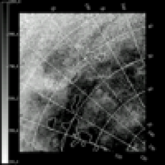
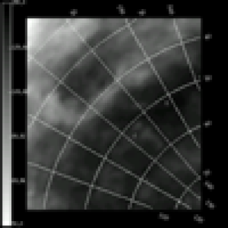
Figure 5: upper panel: The color image shows the observed ROSAT C-band while the contours correspond to the deviation map. The solid contours encircle regions where the modeled intensities are too faint, the dotted contours enclose regions where the model is too bright. Intra-group gas of the M81/M82 group of galaxies within the spectra of the Leiden/Dwingeloo H i survey produces the contour line around $(l,b)\approx(140^{\circ},40^{\circ})$. HVC complex C is located at the bottom, the Lockman hole is surrounded by the dotted contour line on the right hand side. lower panel: The color image shows the modeled ROSAT M-band. The superimposed contours of the corresponding deviation map are almost nonexistent, indicating a quantitatively good model within the uncertainties. Intensities are in $10^{-6}\,$cts s^-1 arcmin^-2.

3.4.1 Testing the two dimensional correlation

To optimize the initial fit parameters (see Sec. 3.3) we compute histograms of the deviation maps and obtain the mean ($\mu$) and variance ($\sigma$). In case of a perfect quantitative correlation between the observation and the model we expect a mean of $\mu=0$ and a variance of $\sigma=1$. This can be achieved by small variations of the free fit parameters and slight changes in the H i column density of the halo component (i.e. the velocity interval of the H i data). It turns out that the quality of the histograms increases when the intensity of the extragalactic background emission is tuned to $(170\pm 90)\cdot 10^{-6}\,{\rm cts\,s^{-1}\,arcmin^{-2}}$ which is fully consistent with Barber et al. (1996) within the uncertainties. After seven iteration steps no further improvement can be achieved. The statistical parameters in the C- and M-band after the optimization are $\mu_{\rm C}=0.13,\sigma_{\rm C}=1.56$ and $\mu_{\rm M}=-0.58,\sigma_{\rm M}=1.12$ respectively. The final C-band model map is shown in Fig. 8 for comparison with the observed C-band intensity distribution (Fig. 5).

3.4.2 The role of $N_{{H\textsc{i}}}$

In order to test which H i components are responsible for the major absorption we use different $N_{\mathrm{HI}}$ maps (see Sect. 2.1). Obviously the smaller the velocity integration interval the lower the $N_{\mathrm{HI}}$ column density. However, the $|v_{\mathrm{LSR}}|\leq 25\,{\rm km\,s^{-1}}$ map does not include the IVC shadows – most obvious for IVC 135+52-45 (Weiß et al. 1999). The X-ray excess emission close to HVC complex C is still present, as well as the deficit of attenuating H i towards the Lockman Hole. Figures 6, 7 and 8 show three model maps of the ROSAT C-band intensity distribution. The maps differ in the amount of H i in the halo component. We calculate the maps for three different LSR velocity intervals: $-25\,{\rm km\,s}^{-1}\leq v_{\rm LSR}\leq+25\,{\rm km\,s}^{-1}$, $-50\,{\rm km\,s}^{-1}\leq v_{\rm LSR}\leq+50\,{\rm km\,s}^{-1}$ and $-70\,{\rm km\,s}^{-1}\leq v_{\rm LSR}\leq+70\,{\rm km\,s}^{-1}$. The model map to the smallest velocity interval has a mean intensity of $I_{\rm C}=(960\pm 360)\cdot 10^{-6}\,{\rm cts\,s^{-1}\,arcmin^{-2}}$. The model map to the medium velocity interval differs by 11 % and the model map to the largest interval by 18 % (see Fig. 6 – 8). From these values we conclude, that most of the CNM and WNM is already included within the smallest velocity range, which is accordingly responsible for the dominant fraction of the absorption. Moreover, the CNM is not present at the positions of low column density (Lockman et al. 1986) and therefore the WNM dominates the absorption of the X-ray radiation. This statistical approach leads to the optimized fit parameters:

$$I_{\rm LHB} = (350\pm 90)\cdot 10^{-6}\,{\rm cts\,s^{-1}\,arcmin^{-2}}$$

$$I_{\rm HALO} = (1380\pm 120)\cdot 10^{-6}\,{\rm cts\,s^{-1}\,arcmin^{-2}}$$

$$I_{\rm EXTRA} = (170\pm 90)\cdot 10^{-6}\,{\rm cts\,s^{-1}\,arcmin^{-2}}$$

$$T_{\rm LHB} = 10^{6.0\pm 0.1}\,{\rm K}$$

$$T_{\rm HALO} = 10^{6.2\pm 0.1}\,{\rm K}.$$

In comparison to Kuntz & Snowden (2000) we only need one single X-ray emitting component for fitting the Galactic halo emission. The temperature we derive is in-between the temperature of the soft and hard component derived by Kuntz & Snowden (2000). The temperature for the LHB component is slightly lower in our case.

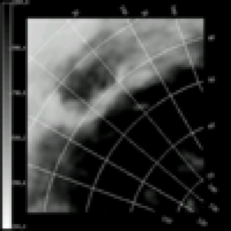
Figure 6: Modeled ROSAT C-band map. The amount of H i corresponds to the velocity interval of $|v_{\rm LSR}|\leq 25$ km s^-1 which does not include the IVC regime. Therefore, the X-ray shadow produced by IVC 135+52-45 (compare to Fig. 5, upper panel) is absent. Intensities are in $10^{-6}\,$cts s^-1 arcmin^-2.

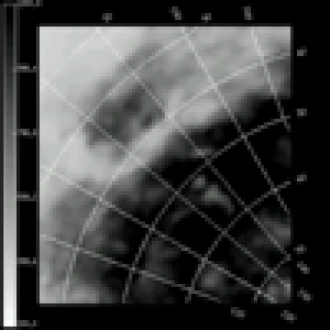
Figure 7: Modeled ROSAT C-band map for the H i velocity interval of $|v_{\rm LSR}|\leq 50$ km s^-1. The mean intensity is about 11% smaller than the one of Fig. 6. Intensities are in $10^{-6}\,$cts s^-1 arcmin^-2.

Figure 8: Modeled ROSAT C-band map for the H i velocity interval of $|v_{\rm LSR}|\leq 70$ km s^-1. The mean intensity is about 18% smaller than the one of Fig. 6. Intensities are in $10^{-6}\,$cts s^-1 arcmin^-2.

It turns out that the entire region around the Lockman Hole $(l,b)=(150^{\circ},53^{\circ})$ is correctly modeled down to the data uncertainties. We can account for the X-ray intensity distribution on a large sky region ($60^{\circ}\times 60^{\circ}$) whereas the Lockman Hole itself is too bright in the model. The question why the model first fails at this prominent position will be discussed in the forthcoming section.

One of the main results is that $T_{\mathrm{LHB}}<T_{\mathrm{HALO}}$. This finding is obvious in the R1/R2 band ratio vs. $N_{\mathrm{HI,h}}$. Because of the strong dependence of the photoelectric absorption on energy ($\sigma\propto E^{-3}$), the soft X-ray photons are much stronger attenuated than the hard ones, leading to an apparent hardening of the X-ray spectrum proportional to $N_{\mathrm{HI}}$. This implies that the higher $N_{\mathrm{HI,h}}$ the lower the R1/R2 band ratio of the $I_{\rm HALO}$ source component. Figure 4 shows the contrary behavior. The higher $N_{\mathrm{HI,h}}$ the larger the R1/R2 band ratio. This finding can only be explained by a cooler LHB plasma with respect to the Galactic halo gas. Using the best fit plasma temperatures we derive an important contribution of the Galactic halo plasma to the observed M-band intensities. The $I_{\rm HALO}$ is about 4 times brighter than $I_{\rm LHB}$ within the ROSAT C-band, while $I_{\rm HALO}\simeq\frac{4}{3}I_{\mathrm{EXTRA}}$ in the ROSAT M-band. $I_{\rm HALO}$ is the dominant source in the ROSAT C- and M-band. We assumed the intensity of the Galactic halo plasma to be constant across the field of interest which is consistent within the uncertainties. The derived fluctuations in halo intensity suggested by Snowden et al. (1994a) may be due to the H i velocity intervals, which differ from our choice. These fluctuations do not appear in our model, since we choose the H i velocity intervals as described above.

4 Specifying the ISM conditions in the Lockman Hole

4.1 Molecular or ionized hydrogen?

As we pointed out in the prior sections, most of the sky region investigated can be explained by our model. The deviating portions of the sky decompose into two types: regions modeled too faint and those modeled too bright. Here we concentrate on the Lockman Hole, which belongs to the latter case (see Fig. 5, upper panel). This is due to a lack of absorbing material. The additional hydrogen column density required to remove the deviation can be estimated to $N_{H\textsc{i}}^{\rm add}\approx(5\pm 3)\cdot 10^{19}\,{\rm cm^{-2}}$.

Since most of the sky region is properly fit by our model, we argue that the ISM towards the Lockman Hole has a different composition to the surroundings. Either the ISM at this particular position contains a molecular gas phase or an ionized gas phase, both of which are detectable as X-ray shadows but not quantitatively traced by the H i data. The H i column density inside the bordering contour lines in Fig. 5 (upper panel) is less than $10^{20}\,{\rm cm^{-2}}$. If we consider a molecular gas phase, a minimum H i column density is needed to shield this molecular phase. Herbstmeier et al. (1993), for example, claimed that an H i column density of at least $3.7\cdot 10^{20}\,{\rm cm^{-2}}$ is needed to allow the formation of molecular hydrogen. From this, we conclude that a molecular gas phase is unlikely to exist. The remaining option is an ionized state of the hydrogen towards the Lockman Hole. Previous studies of the interstellar $H_{\rm\alpha}$ emission towards the Lockman Hole (Hausen et al. 2002) yield $N_{H\textsc{ii}}\approx 2\cdot 10^{19}\,{\rm cm^{-2}}$ which is of the same order of magnitude as $N_{H\textsc{i}}^{\rm add}$. We perform a cross-check of the ionization structure towards the Lockman Hole via far-ultraviolet absorption line measurements by FUSE.

4.2 Far-Ultraviolet absorption line data

In order to investigate the physical conditions of the interstellar medium in the direction of the Lockman Hole we make use of Far-Ultraviolet (FUV) absorption line data. The FUV range bluewards of the Lyman $\alpha$ line and redwards of the Lyman break provides a wealth of spectral diagnostics to study interstellar gas in its various phases (e.g., Savage et al. (2003); Richter et al. (2001a)). A large number of FUV absorption line spectra for almost every direction in the sky is publicly available from the MAST data archive of the Far Ultraviolet Spectroscopic Explorer (http://archive.stsci.edu/fuse/). For the purpose of studying the Lockman Hole field extragalactic background sources such as QSOs and AGNs are favorable in order to ensure a correct continuum placement for the various absorption features, and to include Milky Way halo gas that may contain a significant fraction of the X-ray absorbing neutral and ionized gas in this general direction.

4.3 NGC 3310

From the extragalactic sight lines in the general direction $l\sim 150^{\circ}$, $b\sim 50^{\circ}$ for which good S/N FUSE data is publicly available, we have chosen the one closest to the Lockman Hole: NGC 3310 ($l=156.6^{\circ}$, $b=54.1^{\circ}$). The raw data was extracted using the standard FUSE data reduction pipeline (CALFUSE v.2.1.6), and was then further reduced in a way similar to the data processing procedure described in Wakker et al. (2003). The velocity calibration was made by comparing absorption lines from various atomic and molecular lines with existing H i 21 cm-line data (see below). The FUSE data have an average signal-to-noise ratio (S/N) of $\sim 14$ per resolution element, and a spectral resolution of $\sim 20$ km s^-1 (FWHM).

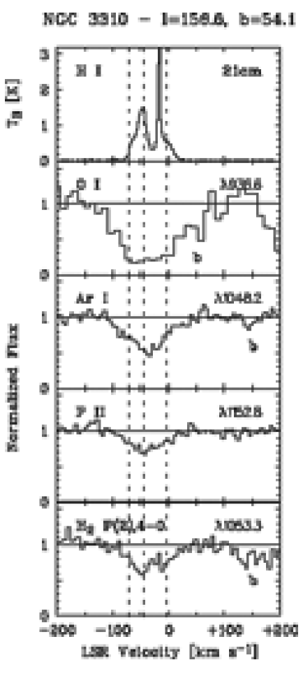
Figure 9: From top to bottom, the panels show the H i 21 cm-line spectrum towards NGC 3310 as measured by the Green Bank Telescope, and the absorption profile of O i, Ar i, P ii, and H₂ P(2),4-0 as measured by FUSE. The dotted lines indicate the LSR velocities $-5,-45,$ and $-70$ km s^-1 (see Sect. 4.3.1 for details).

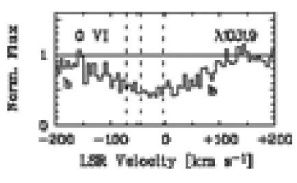
Figure 10: The O vi $\lambda 1031.9$ absorption profile towards NGC 3310 traces the highly ionized gas (see Sect. 4.3.2 for details).

4.3.1 Neutral and weakly ionized gas

In Fig. 9 (uppermost panel) we have plotted the Green Bank H i 21 cm-line spectrum towards NGC 3310 (Murphy et al. 1996) on a LSR velocity scale. The 21 cm-line spectrum shows at least four distinct velocity components: (1) a broad local Galactic component centered at $-11$ km s^-1 with $\log$ N(${H\textsc{i}})=19.63\pm 0.02$, (2) a very narrow local Galactic component at $-17$ km s^-1 having $\log$ N(${H\textsc{i}})=19.54\pm 0.01$, (3) a relatively strong broad component located at $-47$ km s^-1 with $\log$ N(${H\textsc{i}})=19.71\pm 0.01$, related to the Intermediate-Velocity Arch (IV Arch; Wakker (2001)) in the lower Milky Way halo, and (4) a weaker, second IV Arch component at $-65$ km s^-1 with $\log$ N(${H\textsc{i}})=19.11\pm 0.01$. In the lower four panels of Fig. 9 we have plotted the FUSE absorption profiles of O i $\lambda 936.6$, Ar i $\lambda 1048.2$, P ii $\lambda 1152.8$, and H₂ P(2),4-0 $\lambda 1053.3$ in direction of NGC 3310.

Only three velocity components (fitted by Gaussian absorption profiles) are visible in absorption, centered at approximately $-5$, $-45$, and $-70$ km s^-1, in Fig. 9 indicated by dotted lines. Possibly, the two local Galactic components, in the 21 cm-line emission data seen at $-11$ and $-17$ km s^-1, are smearing together into one single absorption component, given the fact the FUSE data has a spectral resolution of only $\sim 20$ km s^-1. However, it is also possible that the narrow $-17$ km s^-1 21 cm-line component relates to gas that partly fills the $21\aas@@fstack{\prime}0$ Green Bank beam, but is not present along the pencil-beam FUSE spectrum towards NGC 3310. Since beam smearing effects can introduce enormous uncertainties when comparing 21 cm-line data with FUV absorption line data for low-column density clouds, it is important to look for possibilities to study the structure of the neutral interstellar gas towards the Lockman Hole based on the FUSE data alone. Unfortunately, the H i Lyman series in the FUSE bandpass cannot be used for this purpose, since these lines are heavily saturated at this column density level.

The Ar i $\lambda 1048.2$ (Fig. 9, third panel) indicates that the bulk of the neutral material resides in the IVC component near $-45$ km s^-1. And also the H₂ absorption (lower-most panel) suggests that most of the diffuse molecular gas is situated in the IV Arch rather than in the local Galactic component (see also Richter et al. (2003) for details on the H₂ spectrum). The best available tracer for the neutral gas in the FUSE bandpass is O i. The O i column density is tightly bound to the H i column density, since both neutral hydrogen and neutral oxygen have the same ionization potential ($13.6$ eV), and their abundance is coupled by charge-exchange reactions. In addition, oxygen is not strongly depleted in dust grains. Unfortunately, O i absorption towards NGC 3310 is saturated for all available lines at $\lambda\geq 930$ Å, and only the relatively weak O i $\lambda 936.6$ can be used to roughly estimate the O i column density. This line is shown in Fig. 9, second panel. As is clearly visible, the O i absorption does not reach the zero-flux level in any of the three absorption components, which (together with the total width of the composite absorption structure) allows upper limits to be placed on the individual equivalent widths and column densities by modeling the component structure with Gaussian absorption components. Such a model also has to account for the H₂ P(3) absorption that partly blends the local Galactic O i absorption component near $+50$ km s^-1 (in Fig. 9 indicated with ‘b’). We have done such modeling for the O i $\lambda 936.6$ line, and find that the O i absorption in the local Galactic component at $-5$ km s^-1 must be $\leq 90$ mÅ  ($3\sigma$ upper limit), while for the two IVC components at $-45$, and $-70$ km s^-1 we find equivalent width limits of $115$ and $85$ mÅ. Assuming that $b=10$ km s^-1 (or greater), these equivalent width limits correspond to logarithmic column density limits of $\leq 16.02$, $\leq 16.57$, and $\leq 15.94$ for O i, and $\leq 19.28$, $\leq 19.83$, and $\leq 19.20$ for H i, respectively, if [O/H] is solar (log (O/H)${}_{\sun}=-3.26$ (Holweger 2001)). Thus, the FUSE data suggest that the H i column density in the local Galactic gas towards NGC 3310 is by a factor of $\sim 2$ lower than indicated by the beam-smeared 21 cm-line data pointed in this direction, while the 21 cm-line matches the FUSE data for the two IVC components. However, unresolved sub-components (particular in the local Galactic component) may be present, in which case these limits could be incorrect.

What does the FUSE spectrum of NGC 3310 tell us about the ionization conditions in the interstellar gas in the direction of the Lockman Hole? As has been demonstrated in earlier studies (Richter et al. 2001b), the P ii/O i column density ratio is a good indicator for the ionization structure in interstellar clouds. P ii has an ionization potential of 19.7 eV, and lives in regions where O and H are both neutral and ionized. Also for phosphorus, dust depletion is not considered to be important. Thus, assuming an intrinsic P/O ratio, the O i and P ii column densities can be used to determine lower limits for the ionization fraction, $f_{\rm ion}=$H${}^{+}/$(H${}^{0}+$H⁺), in the weakly ionized gas phase (for ionization energies $<19.7$ eV). The weak P ii $\lambda 1152.8$ absorption (Fig. 9, fourth panel), can be reproduced by a three–component Gaussian fit, for which the three velocity components have been fixed at $-5$, $-45$, and $-70$ km s^-1. Using this method, we derive equivalent widths of $18\pm 4$ mÅ  for the $-5$ km s^-1 component, $60\pm 8$ mÅ  for the $-55$ km s^-1 component, and $11\pm 4$ mÅ  for the $-70$ km s^-1 component. Assuming a $b$ value of $10$ km s^-1, these equivalent widths correspond to column densities, $\log$ N$({P\textsc{ii}})$, of $12.85\pm 0.10$, $13.51\pm 0.09$, and $12.63\pm 0.14$, respectively. Assuming that all three velocity components have solar phosphorus-to-oxygen abundance ratios (see also Richter et al. 2001a, b), the data for O and P yield $f_{\rm ion}\geq 0.22$ and N(H)=N(H i)+N(H${}^{+})=8.66\times 10^{19}$cm^-2, whereas no useful limits can be obtained for the local Galactic component and the second IVC component, since their P/O column density ratios would allow every degree of ionization (i.e., $f_{\rm ion}\geq 0.0$). The FUSE data therefore indicates that approximately a fifth of the total hydrogen column density in the main IVC component is in ionized form; very likely, the ionization in the local Galactic component is much higher, but the limitations for the FUSE O i data unfortunately does not allow the derivation of a quantitative limit.

4.3.2 Highly ionized gas

The FUSE data also yields information about the highly ionized gas phase for ionization energies $>100$ eV through the two resonance lines of five-times ionized oxygen, O vi, situated at $1031.9$ and $1037.6$ Å. O vi traces collisionally ionized, hot gas at temperatures $T\sim 2\times 10^{5}$ K (thus lower than the X-ray emitting gas), or gas that is photoionized by a hard UV background (or a combination of both). In Fig. 10 we have plotted the O vi $\lambda 1031.9$ absorption profile towards NGC 3310 (the weaker O vi $\lambda 1037.6$ cannot be used due to blending effects). The main analysis of the O vi $\lambda 1031.9$ absorption towards NGC 3310 has already been presented in Wakker et al. (2003) and Savage et al. (2003). O vi absorption is smeared over a broad range from $-200$ to $+90$ km s^-1, thus spanning a velocity range that covers all three velocity components seen in 21 cm-line emission. The total integrated O vi column density is $\log$ N$({O\textsc{vi}})=14.56\pm 0.02$. This column density is slightly (but not significantly) higher than the O vi column densities in other directions outside the Lockman Hole (see Savage et al. 2003). This is not too surprising though, since the pathlength through the Lockman Hole is too short to contribute significantly to the total O vi column density at the expected low volume densities. Assuming that the fraction of oxygen residing in the O vi phase is $\leq 0.2$, the total gas column density of this highly ionized gas phase is $\leq 3.3\times 10^{18}$ cm^-2 for solar oxygen abundances (Holweger 2001). The highly ionized gas component traced by O vi therefore cannot contribute significantly to the total hydrogen gas column density in direction of the Lockman Hole.

5 Conclusion

The analysis performed shows that the main absorption of soft X-rays is due to the WNM. It turns out that a single-temperature plasma in the Milky Way halo is sufficient to reproduce the X-ray distribution on the Lockman Hole field ($60^{\circ}\times 60^{\circ}$) very well. Hence, a patchy Milky Way halo is not likely. Furthermore, the applied fit procedure (simultaneously for four ROSAT energy bands) is very sensitive to temperature. We showed that the temperature of the LHB plasma is lower than the temperature of the halo plasma. The X-ray/H i-analysis of the Lockman Hole itself gives evidence that a large fraction of the attenuating ISM may reside in form of ionized hydrogen.

While the FUSE data of NGC 3310 impressively demonstrates the complex multiphase structure of the gas in the general direction of the Lockman Hole, a precise quantitative analysis of the gas properties turns out to be unfeasible due to the complexity of the velocity structure of the gas that cannot be resolved with the FUSE instrument. The data shows that the majority of the neutral and molecular gas is situated in the IVC component in the lower Milky Way halo rather than in the disk component. Due to the data limitations, we are not able to obtain precise ionization fractions, but the FUSE data of NGC 3310 are at least consistent with the idea of ionized hydrogen in the Lockman Hole. While the ionization fraction is not well constrained by the FUSE data the total amount of ionized gas is sufficiently high to overcome the apparent discrepancy between the H i and X-ray observations.