Recent Microlensing Results from the MACHO Project

Abstract

We describe a few recent microlensing results from the MACHO Collaboration. The aim of the MACHO Project was the identification and quantitative description of dark and luminous matter in the Milky Way using microlensing toward the Magellanic Clouds (LMC and SMC) and the Galactic bulge. We start with a discussion of the Hubble Space Telescope follow-up observations of the microlensing events toward the LMC detected in the first 5 years of the experiment. Using color-magnitude diagrams we attempt to distinguish between two possible locations of the microlensing sources toward the LMC: 1) in the LMC or 2) behind the LMC. We conclude that unless the extinction is extremely patchy, it is very unlikely that most of the LMC microlensing events have source stars behind the LMC. During examination of the HST images of the 13 LMC events we found a very red object next to the source star of event LMC-5. Based on astrometry, microlensing parallax fit and a spectrum, we argue that in this case we directly image the lens – a low-mass disk star.

Then we focus on the majority of the events observed by the MACHO Project, which are detected toward the Galactic bulge. We determine the microlensing optical depth, which describes the amount of matter between us and the Galactic center. We argue that the microlensing optical depth toward the bulge is best measured using only a subclass of the events, namely the ones that have clump giant sources. They are numerous and belong to the brightest stars in the bulge, which makes them insensitive to blending bias. Our analysis of those events suggests that the optical depth toward the Galactic bulge is $\tau_{\rm bulge}=(1.4\pm 0.3)\times 10^{-6}$, in good agreement with other observational constraints and with theoretical models. There are many long-duration events among the bulge candidates. We take advantage of this situation investigating the microlensing parallax effect. We show that the events with the strongest parallax signal are probably due to massive remnants. Events MACHO-96-BLG-5 and MACHO-98-BLG-6 might have been caused by the black holes with masses of order of $6$ solar masses.

¹ Max-Planck-Institut für Astrophysik, Karl-Schwarzschild-Str. 1, 85741 Garching, Germany; e-mail: popowski@mpa-garching.mpg.de

1. The MACHO Microlensing Experiment

The Milky Way is one of the two most massive galaxies in the Local Group and so is likely to represent a typical product of cosmological evolution of matter trapped in a relatively deep potential well. The detailed formation processes of our Galaxy put constraints on cosmology, star formation history, environmental influence on galactic evolution etc. The key to understanding the formation process of the Galaxy is to understand its structure and stellar populations. There are still many questions related to the structure of the Galaxy that have not been satisfactory answered. “What is the Galactic dark halo made off?” is probably the most momentous question but the others related to the inner structure of our Galaxy or the origin of different components also have profound consequences for our understanding of the galaxy formation.

Microlensing is one of the preferred techniques to study the Milky Way because of its sensitivity to both luminous and dark matter. Microlensing results from the bending of light by massive objects. The signal depends sensitively on the alignment between the observer, the source of light (at a distance $D_{s}$), and a lens located between them (at a distance $D_{l}$). Strong signal is observed if at some time the projected distance between the source and the lens is of order of the Einstein radius, $r_{E}$, defined as:

$$r_{E}=\sqrt{\frac{4Gm_{\rm lens}}{c^{2}}\frac{(D_{s}-D_{l})D_{l}}{D_{s}}},$$ (1)

and the event produces significant magnification on a time scale given by

$$t_{E}=\frac{r_{E}}{v_{\perp}},$$ (2)

where $m_{\rm lens}$ is the mass of the lens, and $v_{\perp}$ a relative transverse velocity. The observable quantity, Einstein radius crossing time, $t_{E}$, is a degenerate combination of $m_{\rm lens}$, $v_{\perp}$, $D_{l}$ and $D_{s}$. Fortunately, microlensing phenomenology goes much beyond the simple point lens approximation. The effects of ’parallax’ (Gould 1992; Alcock et al. 1995), binary caustic crossing (Mao & Paczyński 1991; Afonso et al. 2000), or finite source (Gould 1994; Alcock et al. 1997b) allow one to break degeneracies present in the simplest cases and provide useful constraints on stellar physics. Below we will use the effect of parallax, from which one may infer the projected transverse velocity:

$$\tilde{v}=v_{\perp}\frac{D_{s}}{D_{s}-D_{l}}.$$ (3)

Substitution of equations (2) and (3) into (1) results in:

$$M=\frac{c^{2}}{4G}t_{E}^{2}{\tilde{v}}^{2}\frac{D_{s}-D_{l}}{D_{s}D_{l}}\equiv\frac{c^{2}}{4G}t_{E}^{2}\tilde{v}\mu_{\rm rel},$$ (4)

where in the second equity we simply recognized the fact that the relative proper motion of the lens and the source was equal to $\mu_{\rm rel}=v_{\perp}/D_{l}$. When we have $\tilde{v}$ from the parallax fit to the microlensing light curve, then the only uncertainty in the mass comes from the lack of knowledge of the distance to the lens (distance to the source is oftentimes approximately known). With the additional measurement of the relative proper motion, one solves for the mass with no ambiguity.

The amount of mass between the source and observer and its distribution along the line of sight is described by the optical depth, which is the probability that microlensing happens on a given star (typically of order $10^{-7}-10^{-6}$). The actual count of events (microlensing rate) is proportional to the optical depth and to the number of sources. Therefore, microlensing surveys target concentrations of stars to maximize the number of detected events. Microlensing observations toward the LMC and SMC test the existence and composition of the lensing population in the Galactic dark halo. The microlensing optical depth toward the bulge is a function of the matter content of the inner Galaxy and is sensitive to the characteristics of the Galactic model.

Figure 1.: Alcock et al. (2000b) LMC results for the model of standard spherical halo. The plots show the most likely mass of a typical lens $m$ versus the fraction $f$ of the dark halo in MACHOs. The four cases correspond to different cuts and assumptions about the LMC structure.

Less than two decades ago, microlensing was still at a stage of a purely theoretical concept (Paczyński 1986, 1991; Griest 1991). It became such a powerful astrophysical tool thanks to the experiments like the MACHO Survey, which had a major impact on the development and application of the microlensing technique to Galactic studies. The MACHO experiment collected images of the Galactic bulge and Magellanic Clouds from 1992 through 1999. All observations were taken with the 1.3 m Great Melbourne Telescope with a dual-color wide-field camera. The MACHO camera consisted of two sets of four 2k x 2k CCDs that collected blue ($B_{M}$) and red ($R_{M}$) images simultaneously using a dichroic beam splitter. A single observed field covered an area of 43’ by 43’. We observed 82 fields in the LMC, 21 in the SMC and 94 in the Galactic bulge region, and collected about 100000 images. The fields with high priority were observed on most photometric nights in the season. The LMC observations were carried out all year long, whereas the bulge season lasted from March till October. The resulting light curves often contain several hundred points with individual fields sampled on average every few days. Details of the MACHO telescope system are given by Hart et al. (1996) and of the camera system by Stubbs et al. (1993) and Marshall et al. (1994). Details of the MACHO imaging, data reduction and photometric calibration are described by Alcock et al. (1999).

2. Where are the source stars of the LMC events?

We (Alcock et al. 2000b) used two sets of microlensing candidates: conservative set A of 13 events and inclusive set B of 17 events to argue that Massive Compact Halo Objects (MACHOs) contribute of order of 20% to the mass of the dark halo of the Milky Way. Using maximum likelihood technique, we showed that the most likely mass of a typical lens is $\sim 0.5M_{\hbox{$\odot$}}$. Upper limits on the halo contribution of MACHOs consistent with our results were also obtained by the EROS collaboration (Lasserre et al. 2000) based on 3 events in the LMC or 4 events in both Magellanic Clouds. Neither of the groups had enough statistical power to reveal the nature or the location of the lenses along the line of sight. Figure 1 summarizes the MACHO results for a standard model of the Galactic dark halo.

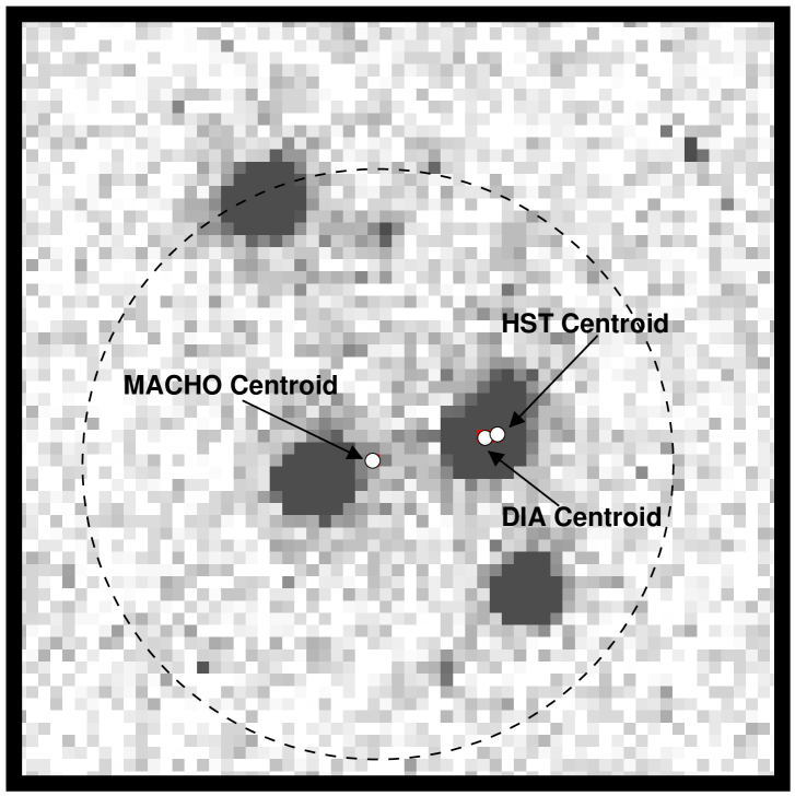
Figure 2.: Illustration of the identification of a microlensing source star with Difference Image Analysis. The circle traced with a dotted line is a typical MACHO seeing disk. The centroid of MACHO light, the centroid of the event source star as inferred from DIA analysis, and the HST centroid of the star closest to this source are marked.

In all cases when we have some additional constraints on the location of the sources, they seem to belong to the known stellar systems (Afonso et al. 2000; Alcock et al. 2001a; Alcock et al. 2001c), which makes some to believe that all of the events must be of this nature. This probability argument is however faulty to some extent. Most effects that give the indication of the lens position occur preferentially when the lens is close to either observer (parallax) or the source (xallarap). Therefore, they provide little information about the location or population membership of the remaining events.

Being unable to conclusively decide on the location of the lenses from available microlensing information, we will now attempt to obtain some indirect bounds. The idea we want to entertain here is the following: find the location of the sources first and then infer the location of the lenses. A useful demonstration of how this works would be to consider two situations with somewhat oversimplified conclusions: 1) sources are in the LMC $\rightarrow$ lenses are in the Milky Way, 2) sources are behind the LMC $\rightarrow$ lenses are in the LMC. The standard case 2) was considered by Zhao, Graff, & Guhathakurta (2000), who placed the source population $\sim 7$ kpc behind the main body of the LMC and assumed uniform LMC extinction of $E(B-V)=0.13$. We will not analyze all the possible locations of the sources and the implications for the lens population here, but we note that this issue is discussed in detail by Alcock et al. (2001b) and Nelson et al. (2003).

The sky appearance at the MACHO observing site at Mount Stromlo is very similar to the one portrayed in “Starry Night”, the oil canvas painted by Vincent van Gogh in Saint–Rémy in 1889. With median seeing above 2 arc-seconds, the individual stars in the LMC are typically not resolved. The objects observed are blends of several stars of different brightness (Alcock et al. 2001b,d). Therefore, we use Hubble Space Telescope (HST) images to construct true color-magnitude diagrams (CMDs) and Difference Image Analysis (DIA) to establish magnitudes and colors of our source stars. The HST and MACHO frames are put on the same astrometric system, and then the centroid of the source star is recovered based on the motion of the centroid of light during the event. The HST star closest to the recovered centroid is assumed to be the source star. This procedure is illustrated in Figure 2. The DIA analysis applied to the entire set A uniquely determines the positions of 12 out of 13 microlensing events. In one case the recovered centroid of source’s light falls exactly in the middle between the two HST stars. Fortunately, they have very similar colors and apparent magnitudes and so we choose one of them at random.

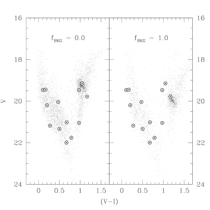
Figure 3.: Color-magnitude diagrams corresponding to two extreme tested models: left one with all microlensing sources in the LMC, and right one with all sources behind the LMC.

Having obtained the unblended characteristics of the source stars of microlensing events we now have to model the source star populations MACHO experiment is sensitive to. We assume that our source stars can be drawn from two population: the bar and disk of the LMC and a background population behind the LMC. We assume that the background population does not differ intrinsically from the one in the LMC. The difference in the CMD appearance comes from additional reddening (here taken to be the mean reddening of stars in the LMC) and the shift in the distance modulus. We start with the HST CMD and convolve it with the MACHO efficiency for detecting stars, which goes to almost zero at $V=22$, and cuts off a substantial fraction of the HST CMD. In this way we reproduce the unblended LMC population observed by the MACHO experiment. The route to mock the background population is more complicated. Each star in the HST CMD must be first shifted by $\Delta(V-I)=E(V-I)=1.38\,E(B-V)=0.18$ mag and $\Delta V=A_{V}+\Delta_{\rm BKG}=0.43+\Delta_{\rm BKG}$ mag, where $\Delta_{\rm BKG}$ is the distance modulus shift of the background population with respect to the LMC. Only then we modify the HST CMD by “filtering” the number of stars through our efficiency curve as in the first case. Based on these pure LMC and background populations, we construct a series of CMDs with a fraction $f_{BKG}$ stars from the background and $(1-f_{BKG})$ from the main body of the LMC. The two extreme cases of $f_{BKG}=0$ and $f_{BKG}=1$ are shown in Figure 3. Spherical symbols with central dots are the sources of the 13 microlensing events, superposed on the underlying population.

We perform a two-dimensional Kolmogorov-Smirnov (KS) test to tell, which models are most consistent with the data. In one dimensional case, a KS test of two samples with number of points $N_{1}$ and $N_{2}$ returns a statistic $D$, defined to be the maximum distance between the cumulative probability functions at any ordinate. Associated with $D$ is a corresponding probability $P(D)$ that if two random samples of size $N_{1}$ and $N_{2}$ are drawn from the same parent distribution a worse value of $D$ will result. This is equivalent to saying that we can exclude the hypothesis that the two samples are drawn from the same distribution at a confidence level of $1.0-P(D)$. If $N_{2}\gg N_{1}$, then this is also equivalent to excluding at a $1.0-P(D)$ confidence level the hypothesis that sample 1 is drawn from sample 2. The concept of a cumulative distribution is not defined in more than one dimension. However, it has been shown that a good substitute in two dimensions is the integrated probability in each of four right-angled quadrants surrounding a given point (Peacock 1983; Fasano & Franceschini 1987). The integrated probability of each quadrant for each distribution is the fraction of data from the distribution which lies in that quadrant. The two dimensional KS statistic $D$ is now taken to be the maximum difference (ranging both over all data points and all quadrants) between the integrated probability of distributions $N_{1}$ and $N_{2}$. The statistic $D$ and the corresponding $P(D)$ are subject to the same interpretation as in the one dimensional case (see Press et al. 1992 for details).

We show the resulting $P(D)$ versus $f_{BKG}$ in Figure 4, where we used the distance modulus shift $\Delta_{\rm BKG}=0.3$. More models are considered by Nelson et al. (2003). Because the creation of the efficiency convolved CMD is a weighted random draw from the HST CMD, the model population created in each simulation differs slightly. This in turn leads to small differences in the KS statistics. The error bars indicate the scatter about the mean value for 20 simulations. We find that the 2-D KS-test probability is highest at a fraction of source stars behind the LMC $f_{BKG}~{}\sim 0.0-0.2$. Most of the features of considered CMDs are almost vertical. As a result, the significant preference for low $f_{BKG}$ arises mostly from the reddening term (see discussion below). In a strict statistical sense, the Kolmogorov-Smirnov test can only be used to reject or confirm the hypothesis that two datasets have a common parent distribution. KS test results do not allow one to draw conclusions about the relative probability, e.g., a KS test probability of 90% does not mean that it is three times as likely that two distributions are identical than if they had returned a KS test probability of 30%. Therefore, Figure 4 should be interpreted with caution. Based on the models analyzed by Nelson et al. (2003), we conclude that the general shape of the KS probability versus $f_{BKG}$ is quite insensitive to the distance modulus displacement.

Figure 4.: Model consistency for different fractions of source stars coming from the background as inferred from a 2-D Kolmogorov-Smirnov test.

We rule out a model in which the source stars all belong to some background population at more than a 95% confidence level (e.g., the KS test probability for the distance modulus displacement of $\Delta_{\rm BKG}=0.3$ for $f_{BKG}>0.9$ is $\sim 0.025$). The less extreme models of the LMC spheroid or stellar shroud self-lensing are not excluded. The allowed region of the $f_{BKG}$ plot ($P>10$%) is consistent with the expected location of the source stars in both the Milky Way lensing and LMC disk+bar self-lensing geometries. However, detailed modeling of the LMC disk+bar self-lensing suggests that it contributes at most 20% of the observed optical depth (Gyuk, Dalal, & Griest 2000). Therefore, the results of the KS test taken together with external constraints, could suggest that the lens population comes mainly from the Milky Way dark halo. This statement, however, would be too strong. Our results are not completely conclusive due to the intrinsic problem of the method. Its serious limitation is the uncertainty in the model of the LMC reddening. The significance of our test will decrease substantially if the average reddening of the LMC is significantly lower or the reddening is very patchy.

3. Direct identification of a microlens

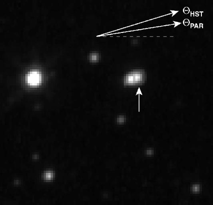
Figure 5.: LMC-5 microlensing event: image showing the lens (arrow) and the source next to it. The arrows in the upper right corner indicate the direction of the lens motion obtained from the parallax fit and HST imaging.

The HST Wide Field Planetary Camera (PC) observations described in the previous section included imaging of the LMC-5 event (Alcock et al. 2001c). Image of this event in HST V, R, and I filters was taken on May 13, 1999, 6.3 years after the peak on February 5, 1993. The system, composed of two objects displaced by 0.134”, was resolved with PC pixels of 0.046” (Figure 5). One of these objects was shown to be a main sequence source stars in the LMC with $V=21.02\pm 0.06$, $(V-R)=0.30\pm 0.09$, and $(V-I)=0.68\pm 0.10$. Its neighbor, marked with an arrow, is a very red, faint object with $V=22.67\pm 0.10$, $(V-R)=1.60\pm 0.12$, and $(V-I)=3.18\pm 0.11$. A chance superposition of such a red object on the LMC source star is of order of $10^{-4}$. Therefore, it is tempting to assume that the red object is the lens. The light curve of event LMC-5 showed very large maximum flux amplification $A_{\rm max}$, which corresponds to very small impact parameter. As a result, we expect that at the peak, the angular distance between the lens and the source was negligible compared to the measured separation. Indeed, for large amplification events the angular distance between the lens and the source is at the peak equal to $4.036\cdot 10^{-4}$” $\!\times A_{\rm max}^{-1}\sqrt{1/x-1}\sqrt{m_{\rm lens}/M_{\odot}}$, where $x=D_{l}/D_{s}$. For LMC-5, the term $A_{\rm max}^{-1}\sqrt{1/x-1}\sqrt{m_{\rm lens}/M_{\odot}}$ is very likely to be $<1$, and, as a result, the lens-source separation at the peak was of order of or smaller than $10^{-3}$ of the current separation. Consequently, the current angular separation is an excellent measure of the relative proper motion between the source and the lens, $\mu_{\rm rel}=0.0214\pm 0.0007$ arcsec/yr with the direction, $\Theta_{\rm rel}=-92^{\circ}$, given by the line connecting the light centroids.

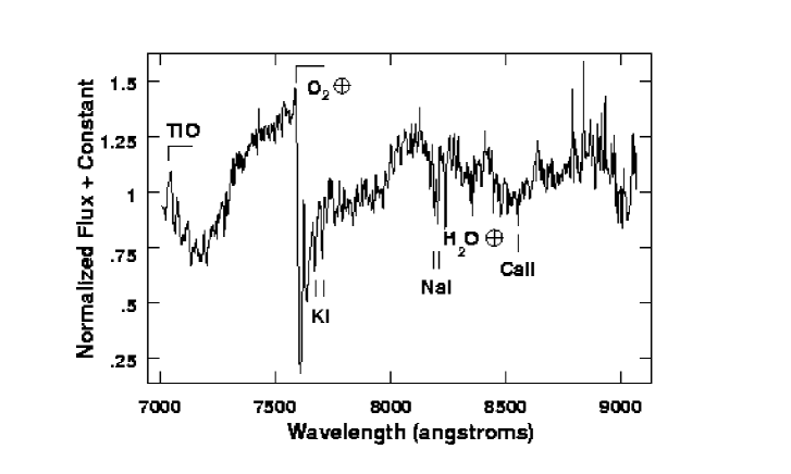
Figure 6.: Blended spectrum of the source and the lens. The red part is dominated by the lens.

Interestingly, LMC-5 has a significant detection of the microlensing parallax effect. We obtained the projected transverse velocity $\tilde{v}=18$ km/s, the direction of lens proper motion, $\Theta_{\rm par}=-97^{\circ}$, and duration $t_{E}=22.5$ days. The agreement between $\Theta_{\rm par}$ and $\Theta_{\rm rel}$ suggests that the red object is indeed the lens for the microlensing event LMC-5. Equation (4) can therefore be used to estimate the mass of the lens $m_{\rm lens}=0.036^{+0.009}_{-0.004}M_{\odot}$, which argues for a sub-stellar object at a very high significance. The errors, however, are not Gaussian and the $3\sigma$ limit on the mass based on the parallax fit is $m_{\rm lens}\leq 0.097M_{\odot}$. In natural units, the relative parallax of the event is $\pi_{\rm rel}=\mu_{\rm rel}/\tilde{v}$. For a nearby lens and a source in the LMC, $\pi_{\rm rel}\approx\pi_{\rm lens}$. This allows us to derive the distance to the lens: $d_{\rm lens}=200^{+40}_{-30}$ pc. Assuming no attenuation of light due to Galactic extinction, we obtain the absolute magnitude of $M^{200{\rm pc}}_{V}=22.67-5.0\log(200{\rm pc}/10{\rm pc})=16.16$.

We took the spectrum of the LMC-5 microlensing system with the European Southern Observatory Very Large Telescope on February 2, 2001 . The separation of the lens-source system at this time was about 0.2”, which was unresolved and resulted in obtaining a composite spectrum (Figure 6). This spectrum becomes more and more dominated by the lens flux as we move redwards of 7000 Å. The presence of KI, NaI, the absence of CsI, RbI, and the TiO band at 7100 Å  coupled with the absence of the VO band at 7450 Å  lead to conclusion that the lens is of spectral type M4-5V. Our HST colors are consistent with this spectral classification (Bessell 1991). According to Cassisi et al. (2000) this spectral type implies $m_{\rm lens}\sim 0.095-0.013M_{\odot}$, which is in $3\sigma$ disagreement with the parallax result.

If the lensing star is an M-dwarf, then it should follow the empirical relation

$$M_{V}=2.89+3.37(V-I)_{0}$$ (5)

derived by Reid (1991). Assuming zero reddening, we obtain $M_{V}=13.61\pm 0.55$ and $d_{\rm lens}=650\pm 190$ pc, again in disagreement with parallax result.

Can the reddening be the reason of this discrepancy? In general:

$$M_{V}=V-5\log\frac{d}{10{\rm pc}}-A_{V}$$ (6)

where $d$ is the distance and $A_{V}$ is the visual extinction, which can be written as $A_{V}=R_{VI}E(V-I)$. Color excess is defined as $E(V-I)\equiv(V-I)-(V-I)_{0}$. Combining equations (5) and (6) for our gravitational lens yields:

$$d_{\rm lens}({\rm pc})=10^{0.2(5.0+V-2.89-3.37(V-I)+(3.37-2.50)E(V-I))}=10^{2.815+0.174\,E(V-I)},$$ (7)

where we assumed a standard value for the selective extinction coefficient $R_{VI}=2.50$. Equation (7) shows that a non-zero extinction would only increase the disagreement between the parallax fit and the spectroscopically motivated estimate of the lens distance (Figure 7). If the lens is not at the very unusual line of sight, then $E(V-I)\sim 0.1$ and correction due to reddening is small, well within the errors of our estimate based on the assumption of zero extinction.

A heliocentric radial velocity of the lens computed using potassium and sodium lines is equal to $v_{\rm rad}=49\pm 10$ km/s. Assuming a distance to the lens and the proper motion inferred from the HST images we solve for the space velocity. At 200 pc, the velocity of the lens relative to the local standard of rest is $U=27$ km/s, $V=-43$ km/s, and $W=-4$ km/s, toward the Galactic center, along rotation, and up out of the plane, respectively. Therefore, the lens has disk-like kinematics. Motivated by the surprisingly faint absolute magnitude implied by the solution based on the parallax fit, Alves & Cook (2001) considered a possibility that the LMC-5 lens is a halo subdwarf. However, since metal-poor stars with disk-like kinematics are very rare, there is a strong indication that the lens belongs to the Galactic disk.

Figure 7.: The distance of the lens as a function of its reddening under the assumption that the lens is an M dwarf that follows the $M_{V}$ – $(V-I)_{0}$ relation of Reid (1991). The non-zero reddening with a standard extinction curve requires larger $d_{\rm lens}$ and so increases the discrepancy between the parallax fit results and photometric constraints that follow from the spectral classification.

The inconsistencies between solutions based on the HST-based proper motion coupled with the MACHO parallax fit on one side and HST photometry coupled with the VLT spectrum on the other might have arisen from difficulty of measuring parallax effect for such a short event. This conflict will be resolved with observations we took on HST Advanced Camera for Surveys. Thanks to a very small pixel size of 0.027”, two epochs of data will allow us to verify the proper motion of the lens and measure the parallactic motion. Despite the described inconsistencies we believe that the red object detected in our images is the lens for the LMC-5 event and that it is a normal low-mass disk star.

4. Microlensing optical depth toward the Galactic bulge

After almost a decade of surveys, the constraints from the Milky Way microlensing observations imposed on the dark matter were so tight (Binney & Evans 2001) that they challenged the standard cuspy dark halo profiles (Navarro, Frenk, & White 1997; Moore et al. 1999). On the other hand, these cuspy profiles are very likely a generic feature of the cold dark matter cosmology. Below we briefly describe the measurements of the optical depth toward the Galactic bulge that led to this situation and proceeded the study described here. In brief, the studies discussed below yield the microlensing optical depth toward the Galactic bulge in the range $\tau_{\rm bulge}=$3$-$4 $\times 10^{-6}$, 2$-$3 times higher than implied by other observational constraints and theoretical models. Udalski et al. (1994) found 9 events in the first two year of the Optical Gravitational Lensing Experiment (OGLE) data. They set the lower limit on the optical depth to the Galactic bulge at $\tau_{\rm bulge}=(3.3\pm 1.2)\times 10^{-6}$. The uncertainties in this study were related to the detection efficiency analysis as well as small number statistics. Alcock et al. (1997a) described a set of 45 bulge events. They computed the so called sampling efficiencies, which are a good approximation only for bright events. Therefore, unbiased analysis could have been done only for 13 clump giants, which resulted in large uncertainties of the optical depth ($\tau_{\rm bulge}=3.9^{+1.8}_{-1.2}\times 10^{-6}$). Udalski et al. (2000) presented a catalog of over 200 microlensing events from the last 3 seasons of the OGLE-II bulge observations. Woźniak et al. (2001) released another catalog of about 500 events selected using image subtraction technique. Unfortunately, no efficiency analysis has been done for these two samples of OGLE events so the information that can be extracted from them is very limited. Alcock et al. (2000a) performed Difference Image Analysis of three seasons of bulge data in 8 frequently sampled MACHO fields and found 99 events. They determined $\tau_{\rm bulge}=3.23^{+0.52}_{-0.50}\times 10^{-6}$ at $(l,b)=(2\hbox{$.\!\!^{\circ}$}68,-3\hbox{$.\!\!^{\circ}$}35)$. This was a major development in bulge microlensing. The DIA technique resulted in a substantial improvement in photometry, so this analysis was less vulnerable to uncertainties in the parameter determination. However, there are two potential problems with this analysis. First, the detection efficiency estimate suffers from the fact that a deep HST luminosity function was available for only one field. Second, the lensed sources are not guaranteed to be in the Galactic bulge. The measured optical depth is, therefore, converted to the optical depth toward the bulge using a fudge factor. Popowski (2002) showed that the reasonable modification of this factor alone can lower the estimate of the optical depth by almost 20%. To cure this uncomfortable situation we would like to select the event that have sources in the bulge. Events with clump giants as sources are excellent candidates, since clump giants are among the brightest and most numerous stars in the bulge. Being bright, clump sources have an additional nice feature – they are almost unaffected by blending.

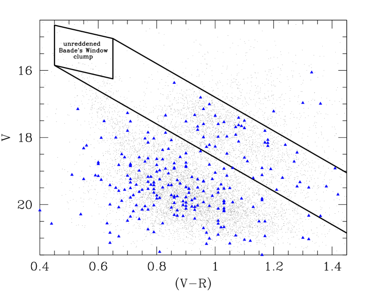
Figure 8.: The locus of clump giants in a color-magnitude diagram can be obtained by shifting the locus of unreddened clump population at the Galactic bulge distance along the reddening line. Here we show the clump region obtained under the assumption that the coefficient of selective extinction $A_{V}/E(V-R)=5.0$.

Blending is a major problem in any analysis of the microlensing data involving point spread function photometry. The bulge fields are crowded, so that the objects observed at a certain atmospheric seeing are blends of several stars. At the same time, typically only one star is lensed. This complicates a determination of the events’ parameters and the analysis of the detection efficiency of microlensing events. If the sources are bright one can avoid these problems. First, a determination of parameters of the actual microlensing events becomes straightforward. Second, it is sufficient to estimate detection efficiency based on the sampling of the light curve alone. This eliminates the need of obtaining deep luminosity functions across the bulge fields. Therefore, in this discussion we concentrate on the events where the lensed stars are clump giants (Popowski et al. 2001a,b). We are using the results of the analysis performed on five seasons of data (1993–1997) in 77 fields.

Figure 9.: The location of the analyzed MACHO fields (square regions) with the location of the clump events (circles). The size of each circle is proportional to the duration of the event. Note the concentration of long events in field 104 at $(l,b)=(3\hbox{$.\!\!^{\circ}$}1,-3\hbox{$.\!\!^{\circ}$}0)$.

The events with clump giants as sources have been selected from the sample of all events. The procedure that leads to a selection of microlensing events of general type consists of several steps. First, all the recognized objects in all fields are tested for any form of variability. Second, a microlensing light curve is fitted to all stars showing any variation and the objects that meet very loose selection criteria (cuts) enter the next phase. Here, this selection returns almost 43000 candidates. These candidates undergo more scrutiny and are subject to more stringent cuts, most of which test for a signal-to-noise of the different parts of the light curve. Here, this last procedure narrows a list of candidate events to $\sim 280$. The question, which of those sources are clump giants, is investigated through the analysis of the global properties of the color-magnitude diagram in the Galactic bulge. Using the accurately measured extinction towards Baade’s Window (Stanek 1996 with zero point corrected according to Gould, Popowski, & Terndrup 1998 and Alcock et al. 1998) allows us to locate bulge clump giants on the dereddened color-magnitude diagram. Such diagram can be then used to predict the positions of clump giants on the color-apparent magnitude diagram for fields with different extinction. Based on Baade’s Window data we conclude that unreddened clump giants are present in the color range $(V-R)_{0}\in(0.45,0.65)$, where they concentrate along a line $V_{0}=14.35+2.0\,(V-R)_{0}$. We assume that the actual clump giants scatter in $V_{0}$-mag around these central values, but by not more than 0.6 mag toward both fainter and brighter $V_{0}$. This defines the parallelogram-shaped box in the upper left corner of Figure 8. With the assumption that the clump populations in the whole bulge have the same properties as the one in the Baade’s Window, the parallelogram described above can be shifted by the reddening vector to mark the expected locations of clump giants in different fields. The solid lines are the boundaries of the region where one could find the clump giants in fields with different extinctions. There are a few more $V$-mag and $(V-R)$-color cuts that determine the final shape of the clump region. Several assumptions that went into creating this region should be carefully reviewed. For example, the assumed spread in $V$ magnitudes can be either bigger or smaller or asymmetric around the central value, clump giants in different fields may have different characteristics etc. In retrospect, we conclude that the effect of the uncertainty in the selective extinction coefficient $R_{VR}$ is probably the hardest to deal with. The clump region from Figure 8 contains 52 unique clump events from the five bulge seasons discussed here. Their location in Galactic coordinates is shown in Figure 9, superposed on the outlines of the analyzed MACHO fields. The size of each circle is proportional to the duration of the event.

Based on this sample of events we estimate the bulge optical depth from the following formula:

$$\tau=\frac{\pi}{2NT}\sum_{\small\rm all\;events}\frac{t_{E}}{\epsilon(t_{E})},$$ (8)

where $N$ is the number of observed stars (here about 2.1 million clump giants), $T$ is the total exposure (here about 2000 days) and $\epsilon(t_{E})$ is an efficiency for detecting an event with a given $t_{E}$. The sampling efficiencies were obtained with the pipeline that has been previously applied to the LMC data (for a description see Alcock et al. 2001d). In brief, artificial light curves with different parameters have been added to 1% of all clump giants in the 77 considered fields and the analysis used to select real events was applied to this set. For a given duration of the artificial event, the efficiency was computed as a number of recovered events divided by a number of input events. The efficiencies used in this analysis are global efficiencies averaged over clump giants in all 77 fields. The optical depth is reported at the central position that is an average of positions of 1% of the analyzed clump giants. We obtain:

$$\tau_{\rm bulge}=(2.0\pm 0.4)\times 10^{-6}\;\;\;\;\;{\rm at}\;\;\;\;\;(l,b)=(3\hbox{$.\!\!^{\circ}$}9,-3\hbox{$.\!\!^{\circ}$}8).$$ (9)

with the error computed according to the formula given by Han & Gould (1995). In Figure 10 we plot the spatial distribution of the optical depth. The variation of the optical depth is dominated by the Poisson noise. The gradient of the optical depth is stronger in $b$ than in $l$. About 40% of the optical depth is in the long events with $t_{E}>50$ days. Such a population of long events is not easily explained by the standard models of Galactic structure and kinematics. Field 104 at $(l,b)=(3\hbox{$.\!\!^{\circ}$}1,-3\hbox{$.\!\!^{\circ}$}0)$ has the largest number of clump events (10) and the optical depth of $(1.4\pm 0.5)\times 10^{-5}$.

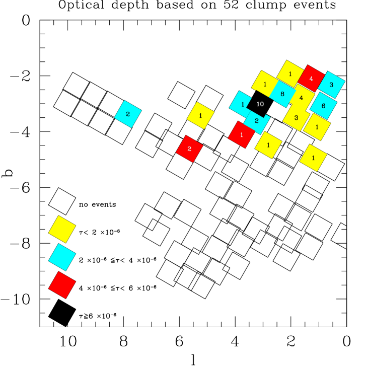
Figure 10.: Field-by-field optical depth. The shades correspond to different ranges in the optical depth. The numbers of events are given in the center of each field. White fields with no numbers have no detected events. The errors in the optical depth are dominated by the Poisson noise. Note the high optical depth in field 104 at $(l,b)=(3\hbox{$.\!\!^{\circ}$}1,-3\hbox{$.\!\!^{\circ}$}0)$.

There is a high concentration of long-duration events in this field (5 out of 10 events longer than 50 days are in 104, including the longest 2). We investigate how statistically significant is this concentration. The analysis of event durations uncorrected for efficiencies provides a lower limit on the difference between the frequently-sampled field 104 and all the remaining clump giant fields. We use the Wilcoxon’s number-of-element-inversions statistic (see Popowski et al. 2001a for a description). The Wilcoxon’s statistic is equal to 320, whereas the expected number is 210 with an error of about 43. Therefore the events in 104 differ (are longer) by $2.55\sigma$ from the other fields. That is, the probability that events in 104 and other fields originate from the same parent population is of order of 0.011. Popowski’s (2002) analysis of the DIA events from Alcock et al. (2000a) confirms this duration difference. We conclude that field 104 is anomalous both in terms of the optical depth and duration distribution. Both effects can be explained simultaneously by the concentration of mass along this line of sight.

The currently available Galactic models are smooth on the scales of a single MACHO field. Therefore, they cannot account for such a localized anomalous behavior as in field 104, and it seems justified to remove this field as an outlier. With this modification, the optical depth decreases to $\tau_{\rm bulge}=(1.4\pm 0.3)\times 10^{-6}$, which is $2/3$ of its original value, and becomes fully consistent with infrared-based models of the Galactic bar (Bissantz & Gerhard 2002, Evans & Belokurov 2002). This lower optical depth is supported by the very recent determination from the EROS group by Afonso et al. (2003), who report $\tau_{\rm bulge}=(0.94\pm 0.29)\times 10^{-6}$ based on 16 clump events in fields centered on $(l,b)=(2\hbox{$.\!\!^{\circ}$}5,-4\hbox{$.\!\!^{\circ}$}0)$. Surprisingly, another recent determination of the optical depth by the MOA collaboration (Sumi et al. 2002), based on 28 events recovered with DIA technique, gives the high optical depth of $\tau_{\rm bulge}=3.36_{-0.81}^{+1.11}\times 10^{-6}$. This value compares very well with the DIA result of Alcock et al. (2000a). In conclusion, there is no longer a general discrepancy between the microlensing observations and Galactic models. Instead, there is a puzzling gap between the optical depth measurements based on clump events and the samples from the Difference Image Analysis technique.

5. Stellar remnants as gravitational microlenses

Equations (1) and (2) show that durations of microlensing events could in principle be a good probe of lens masses. However, event’s duration depends also on the kinematics of populations involved in the lensing process. As nicely showed by Gould (2000; Figure 1), the duration distribution is very wide even for a population of lenses with a single mass. Therefore, despite the fact that $\sim 20$ % of events may be due to remnants in the form of white dwarfs, neutron stars and black holes, one cannot use just durations to identify this population. Events showing parallax effect (equation 4) are in high demand as they provide very stringent constraints on the lens masses.

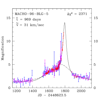
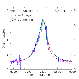
Figure 11.: Light curves of two microlensing events with likely black hole lenses. The data come from the MACHO project and several sources of follow-up observations. The improvement of the parallax fit (solid curve) over the standard fit (dashed curve) is easily visible.

We present the analysis of the longest timescale microlensing events with $t_{E}>70$ days (Bennett et al. 2002). We used the MACHO experiment data described in §1 as well as the follow up data from the MACHO/GMAN observations on the CTIO 0.9 m telescope (Becker 2000) and from the MPS Collaboration on the Mount Stromlo 1.9 m telescope (Rhie et al. 1999). We performed parallax fit to over 300 events detected by MACHO toward the Galactic bulge. We considered parallax signal to be reliable when the difference in the goodness of fit between the standard microlensing curve and the parallax fit was $\Delta\chi^{2}\geq 200$. This selection criterion returned 6 events: 104-C, 96-BLG-5, 96-BLG-12, 98-BLG-6, 99-BLG-1, and 99-BLG-8. The light curves and microlensing fits for the two microlensing events with likely black hole lenses, 96-BLG-5 and 98-BLG-6, are presented in Figure 11.

The CMD analysis of the events indicates that MACHO-104-C and MACHO-96-BLG-12 source stars are bulge clump giants. Source star for MACHO-99-BLG-8 is likely a bulge giant. MACHO-96-BLG-5 is likely a blended main sequence star. The CMD locations of MACHO-98-BLG-6 and MACHO-99-BLG-1 source stars suggest that they can be either bulge subgiant stars or red clump giants in the Sgr dwarf galaxy. However, their radial velocities of $v_{\rm rad}=-65\pm 2$ km/s and $v_{\rm rad}=64\pm 2$ km/s, respectively are not consistent with the radial velocity of Sgr dwarf $v_{\rm rad}^{\rm SGR}=140\pm 10$ km/s (Ibata et al. 1997). Therefore, we concluded that they must have bulge sources.

Figure 12.: Mass versus distance relations for two microlensing events with likely black hole lenses (solid lines). The likelihood functions computed using a standard Galactic model are shown as long-dashed lines. The short-dashed line gives a lower limits on the distance to the lens assuming that the lens is a main sequence star. Such a case is particularly unlikely for event 96-BLG-5.

The 6 parallax events have $\tilde{v}$ in the range $30-80$ km/s. If we were to assume that the bulge and disk velocity dispersions are negligible in comparison with the Galactic rotation of about 200 km/s, then, for the disk lenses, equation (3) would imply that $D_{l}=D_{s}\tilde{v}/(200{\rm\,km/s}+\tilde{v})$. For the sources in the bulge at $D_{s}\approx 8$ kpc and our measured $\tilde{v}$ this would result in the distances of the lenses between about 1 kpc and 2.3 kpc. In reality, the bulge and disk velocity dispersions modify this result to some extent, but this example shows how we can obtain constraints on the lens distance (and consequently mass) from kinematics of Galactic populations. Here we assume that the stellar remnants have the same kinematics and density distributions as the observed stellar populations. To construct likelihood functions of the lens distance given its $\tilde{v}$, we assume for the density profiles a standard double exponential disk and barred bulge of Han & Gould (1996). Our model disk has an isotropic velocity dispersion of 30 km/s, and a flat rotation curve of 200 km/s. The bulge is non-rotating and has an isotropic velocity dispersion of 80 km/s. The resulting likelihood curves are shown in Figure 12 as dotted lines for the two parallax events with the highest predicted lens masses. The solid line is a graphic representation of equation (4) under the assumption that the sources are in the bulge at $D_{s}=8$ kpc. Following the Bayesian method and assuming a uniform prior, we may interpret our likelihood function as a probability distribution of a certain lens mass, which allows us to determine the uncertainty in mass estimation.

We may obtain an additional constraint on the lens distances and masses if we assume that they are main sequence stars. This is achieved by finding the upper limit on the lens brightness. To this end, we use the blending fraction derived from the parallax fit. For our two best candidates: the main sequence lens is extremely unlikely for MACHO-96-BLG-5; for MACHO-98-BLG-6, the main sequence lens is not excluded and its most likely distance is about 6.1 kpc. These additional constraints are depicted in Figure 12 by short-dashed lines.

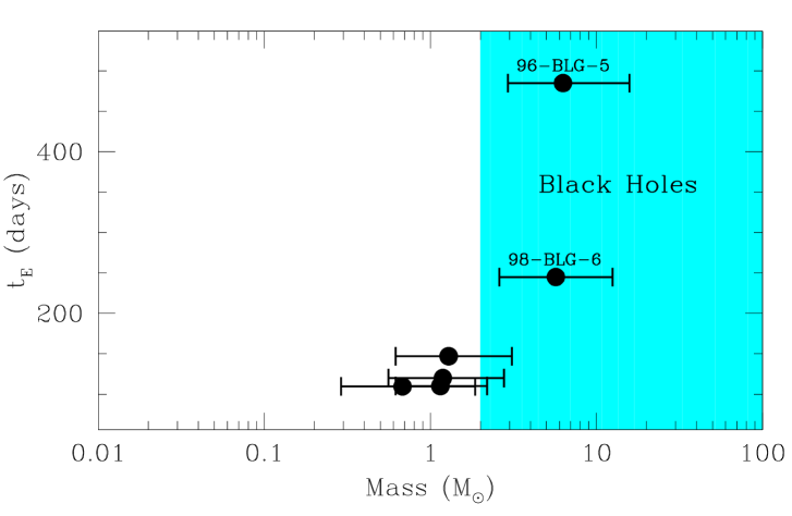
Figure 13.: Event duration versus the lens mass for the 6 events with strong parallax signal. One sigma error bars are shown.

In Figure 13 we present the mass estimates for 6 bulge events with strong detections of the parallax signal. The region of likely black holes, i.e., the lenses with masses larger than $2M_{\odot}$ (Akmal, Pandharipande, & Ravenhall 1998) is shaded. The 95% lower limits on the masses of two candidates that fall into this region are: 1.64 $M_{\odot}$ for MACHO-96-BLG-5 and 0.94 $M_{\odot}$ for MACHO-98-BLG-6. Therefore, in principle both of them could be neutron stars and for MACHO-98-BLG-6 even the main sequence star is a possibility. But we note that the measured neutron stars masses are close to the Chandrasekhar mass, $M_{NS}=1.35\pm 0.04M_{\odot}$ (Thorsett & Chakrabarty 1999). Such masses are excluded for MACHO-96-BLG-5 at more than 95% confidence and for MACHO-98-BLG-6 at more than 90% confidence, which makes them excellent black hole candidates. We obtain similar conclusions when we generalize our likelihood function to include the lens mass function prior as suggested by Agol et al. (2002), but the results are very sensitive to the assumed mass function.

Together with MACHO-99-BLG-22/OGLE-1999-BUL-32 (Mao et al. 2002), the lenses of these events are the first candidates for black holes detected without observations of matter bound to the black hole. These 2 (3) events come from the considered sample of around 300 events, thus constituting around 1% of all events. However, they have very long durations, and contribute substantially more to the total amount of mass along the line of sight. If all three events are causes by black hole lenses, then the stellar mass fraction of black holes may be as high as 10%. This in turn would suggest that most of the black holes are not observed as X-ray binary systems.

6. Summary

We described four separate investigation into the nature of microlenses and Galactic structure based on the microlensing events detected by the MACHO collaboration. Briefly:

1. We compared the color-magnitude location of the source stars for the LMC events with composite CMDs representing different lensing scenarios. If extinction is not too patchy, then it is unlikely that most of the microlensing events in the LMC have source stars behind the LMC.

2. We performed a detailed analysis of event LMC-5 from 1993, which in 1999 was resolved into 2 stars in the HST images. We identified one of them as a source and another as a lens. The lens is a low-mass member of the Galactic disk. Its mass $m_{\rm lens}$ is somewhat uncertain, but likely in the range between $0.04$ and $0.13\,M_{\odot}$.

3. We described the problem of the microlensing optical depth toward the Galactic bulge. From clump giant events, we obtained $\tau_{\rm bulge}=(2.0\pm 0.4)\cdot 10^{-6}$ when we averaged over 77 MACHO fields and $\tau_{\rm bulge}=(1.4\pm 0.3)\cdot 10^{-6}$ when a single highly anomalous field was excluded. Therefore, we showed that the results from clump giants are no longer in disagreement with infrared-based models of the Galactic bar. The situation is, however, still complicated due to the fact the Difference Image Analyses result in substantially higher optical depths. This difference is not understood.

4. We found several events that show clear signs of parallax effect in their light curves, and we selected the six strongest candidates. The average mass of the lenses of these events is 2.7 solar masses. The two longest events may be due to black holes with $M_{\rm bh}$ of order of 6 solar masses. It is very likely that the long-duration events toward the Galactic bulge are caused by massive remnants.

Acknowledgments.

This work was performed under the auspices of the US Department of Energy, National Nuclear Security Administration, by the University of California, Lawrence Livermore National Laboratory, under contract W-7405-ENG-48. PP thanks the conference organizers for invitation to this exciting meeting.

References

Agol, E., Kamionkowski, M., Koopmans, L.V.E., & Blandford, R.D. 2002, ApJ, 576, L131

Afonso, C., et al. 2000, ApJ, 532, 340

Afonso, C., et al. 2003, A&A, accepted (astro-ph/0303100)

Akmal, A., Pandharipande, V.R., & Ravenhall, D.G. 1998, Phys. Rev. C, 58, 1804

Alcock, C., et al. 1995, ApJ, 454, L125

Alcock, C., et al. 1997a, ApJ, 479, 119

Alcock, C., et al. 1997b, ApJ, 491, 436

Alcock, C., et al. 1998, ApJ, 494, 396

Alcock, C., et al. 1999, PASP, 111, 1539

Alcock, C., et al. 2000a, ApJ, 541, 734

Alcock, C., et al. 2000b, ApJ, 542, 281

Alcock, C., et al. 2001a, ApJ, 552, 259

Alcock, C., et al. 2001b, ApJ, 552, 582

Alcock, C., et al. 2001c, Nature, 414, 617

Alcock, C., et al. 2001d, ApJS, 136, 439

Alves, D.R. & Cook, K.H. 2001, AAS, 199.1613

Becker, A.C. 2000, Ph.D. thesis, Univ. Washington

Bennett, D.P., et al. 2002, ApJ, 579, 639

Bessell, M.S. 1991, AJ, 101, 662

Binney, J.J, & Evans, N.W. 2001, MNRAS, 327, L27

Bissantz, N., & Gerhard, O. 2002, MNRAS, 330, 591

Cassisi, S., Castellani, V., Ciarcelluti, P., Piotto, G. & Zoccali, M. 2000, MNRAS, 315, 679

Evans, N. W., & Belokurov, V. 2002, ApJ, 567, L119

Fasano, G., & Franceschini, A. 1987, MNRAS, 225, 155

Gould, A. 1992, ApJ, 392, 442

Gould, A. 1994, ApJ, 421, L71

Gould, A., Popowski, P., & Terndrup, D.T. 1998, ApJ, 492, 778

Gould, A. 2000, ApJ, 535, 928

Griest, K. 1991, ApJ, 366, 412

Gyuk, G., Dalal, N., Griest, K. 2000, ApJ, 535, 90

Han, C, & Gould, A. 1995, ApJ, 449, 521

Han, C, & Gould, A. 1996, ApJ, 467, 540

Hart, J., et al. 1996, PASP, 108, 220

Ibata, R.A., Wyse, R.F.G., Gilmore, G., Irwin, M.J., & Suntzeff, N.B. 1997, AJ, 113, 634

Lasserre, T., et al. 2000, A&A, 355, L39

Mao, S., & Paczyński, B. 1991, ApJ, 374, L37

Mao, S., et al. 2002, MNRAS, 329, 349

Marshall, S.L., et al. 1994, in IAU Symp. 161, Astronomy From Wide Field Imaging, ed. H.T. MacGillivray, et al., (Dordrecht: Kluwer)

Moore, B., Ghigna, S., Governato, F., Lake, G., Quinn, T., Stadel, J., Tozzi, P. 1999, ApJ, 524, L19

Navarro, J.F., Frenk, C.S., & White, S.D.M. 1997, ApJ, 490, 493

Nelson, C.A., et al. 2003, AJ, submitted

Paczyński, B. 1986, ApJ, 304, 1

Paczyński, B. 1991, ApJ, 371, L63

Peacock, J.A. 1983, MNRAS, 202, 615

Popowski, P., et al. 2001a, in ASP Conference Series 239, Microlensing 2000: A New Era of Microlensing Astrophysics, eds. J.W. Menzies and P.D. Sackett (San Francisco: Astronomical Society of the Pacific), 244 (astro-ph/0005466)

Popowski, P. et al. 2001b, in ASP Conference Series 245, Astrophysical Ages and Times Scales, eds. T. von Hippel, C. Simpson, & N. Manset (San Francisco: Astronomical Society of the Pacific), 358 (astro-ph/0202502)

Popowski, P. 2002, MNRAS, submited (astro-ph/0205044)

Press, W.H., Teukolsky, S.A., Vetterling, W.T., & Flannery, B.P. 1992, Numerical Recipes in C, Second Edition

Reid, N. 1991, AJ, 102, 1428

Rhie, S.H., Becker, A.C., Bennett, D.P., Fragile, P.C., Johnson, B.R., King, L.J., Peterson, B.A., & Quinn, J. 1999, ApJ, 522, 1037

Stanek, K.Z. 1996, ApJ, 460, L37

Stubbs, C.W., et al. 1993, in Proceedings of the SPIE, Charge Coupled Devices and Solid State Optical Sensors III, ed. M. Blouke, 1900.

Sumi, et al. 2002, ApJ, accepted (astro-ph/0207604)

Thorsett, S.E. & Chakrabarty, D. 1999, ApJ, 512, 288

Udalski, A., et al. 1994, Acta Astron., 44, 165

Udalski, A., et al. 2000, Acta Astron., 50, 1

Woźniak, P., et al. 2001, Acta Astron., 51, 175

Zhao, H., Graff, D.S., & Guhathakurta, P. 2000, ApJ, 532, L37