Simulations of Evolving or Outbursting Molecular Protostellar Jets

Abstract

The kinematic and radiative power of molecular jets is expected to change as a protostar undergoes permanent or episodal changes in the rate at which it accretes. We study here the consequences of evolving jet power on the spatial and velocity structure, as well as the fluxes, of molecular emission from the bipolar outflow. We consider a jet of rapidly increasing density and a jet in which the mass input is abruptly cut off. We perform three dimensional hydrodynamic simulations with atomic and molecular cooling and chemistry. In this work, highly collimated and sheared jets are assumed. We find that position-velocity diagrams, velocity-channel maps and the relative H₂ and CO fluxes are potentially the best indicators of the evolutionary stage. In particular, the velocity width of the CO lines may prove most reliable although the often-quoted mass-velocity power-law index is probably not. We demonstrate how the relative H₂ 1–0 S(1) and CO J=1–0 fluxes evolve and apply this to interpret the phase of several outflows.

1 Introduction

Jets are being increasingly associated with protostars and with bipolar molecular outflows. Prominent examples of jet-driven collimated outflows include HH 111 (Nagar et al., 1997; Hartigan et al., 2001), HH 211 (Gueth & Guilloteau, 1999; Chandler & Richer, 2001), HH 212 (Lee et al., 2000) and HH 288 (Gueth et al., 2001). For many other outflows, there is evidence that their momentum is also derived from the thrust of jets. For example, transverse shock structures behind bow shocks are interpreted as the sites of jet impact (Smith et al., 2003). Nevertheless, estimated jet thrusts appear insufficient to drive some outflows (Fridlund & Liseau, 1998) and ballistic bullets and wide winds have been invoked. Alternatively, as investigated here, the presently observed jet may not reflect the ancestor jet that has previously driven the outflow.

Our goal is to determine the observable characteristics of outflows driven by molecular jets with evolving mass flow rates. Jet evolution was considered as an interpretation of the systematic decrease in flow velocity with distance in the atomic HH 34 outflow (Cabrit & Raga, 2000). The deduced requirements appeared unlikely and an alternative precessing-fragmenting scenario was favoured. A systematically increasing jet speed was simulated by Lim et al. (2002). Their idea was to explain how molecules can be accelerated to high speed without destruction. Here, we choose to evolve the mass flow rate rather than the speed since it is clear that the mass flow rate must change by many orders of magnitude as a protostar evolves. The taxonomy of protostars is defined by the categories Class 0 through Class 3, which have been linked to an evolutionary sequence (Lada, 1987; Andre et al., 1993). One scenario connects this sequence to simultaneous evolutions in both the accretion rate and the outflow rate (Smith, 2000). Furthermore, certain protostars undergo outbursts (Narayanan & Walker, 1996), the consequences of which may also show up later in the outflow properties (Arce & Goodman, 2001).

We investigate a limited set of three-dimensional simulations that correspond to significant and permanent changes to the input mass flux. This complements studies of outflow development generated by non-evolving heavy molecular jets (Suttner et al., 1997; Davis et al., 1998; Völker et al., 1999) as well as a range of jet conditions (Rosen & Smith, 2003). We first consider a rapid decrease in the mass flux, which we suspected would produce a bullet-like outflow. A decrease in mass flux of some variety must accompany the transitional stages of a protostar into a star. In addition, we model a jet that increases density after some initial propagation, and this model correlates with the opposite end of a protostar’s evolution. During the initial collapse of the core into a protostellar disk, a very young jet must ignite and, therefore, be characterised by an increase in mass flux.

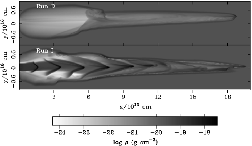
Figure 1: Midplane cross sections of density. These are cross sections for z/R_j = 0.0 of Run D at t = 1300 yr (top) and Run I at t = 1400 yr (bottom). Each is scaled to the same maximum and minimum and the scale, with darker shading indicating denser regions, is displayed below the cross sections. The complete computational domain in the two axes is displayed. In both panels, the vertical axis is the $y$-axis.

Certain features of the molecular line emission from outflows have been attributed to an evolving jet mass outflow rate. For example, it is believed that the energy radiated from shock waves provides a measure of the present driving power while the mechanical luminosity provides a record of the driving history. In this way, the ratio of emissions from vibrationally excited molecular hydrogen and rotationally excited carbon monoxide could determine the evolutionary phase of the protostellar exhausts (Davis et al., 1998; Yu et al., 2000). We can determine here the validity of this statement, although these simulations are of a particular type and scale and so only begin to illustrate the full range of possibilities. For example, we take here a hydrodynamic highly-collimated jet and a uniform ambient medium that are both initially fully molecular. In the next section, we discuss more fully the characteristics of the jet simulations.

2 ZEUS-3D with Molecular Cooling and Chemistry

2.1 The code

We have modified the ZEUS-3D code, which usually updates variables with an explicit method, to include a semi-implicit method that calculates the molecular and atomic hydrogen fractions, according to the prescription of Suttner et al. (1997). We have also added a limited equilibrium C and O chemistry to calculate the CO, OH and H₂O abundances (Rosen & Smith, 2003). Equilibrium CO and H₂O is a reasonable estimate at high density, consistent with the low numerical resolution of the cooling layers behind shock waves (Rosen & Smith, 2003).

The details of the many components of the cooling function and chemistry network are discussed in the appendices of Smith & Rosen (2003). As an overview, we include cooling through rotational and vibrational transitions of H₂, CO, and H₂O, H₂ dissociative cooling and reformation heating, gas-grain cooling/heating, and a time-independent atomic cooling function that includes non-equilibrium effects. We include an additional 10% by number of helium atoms, so the mean particle mass is 2.32 $\times$ 10^-24 g. The dust temperature is fixed at 20 K.

The ZEUS code suffers from numerical errors. Recently, Falle (2002) has explored the appearance of rarefaction shocks which, as the name suggests, are particularly resistant and their influence cannot be removed by increasing the resolution. They may occur in locations where the local Courant number is near 0.5 and where the velocity is negative. Inaccurate fluid patterns could result for adiabatic or MHD flows but isothermal flows are not significantly in error. The present jet simulations are thus immune to these errors, with strong forward motion and strong cooling, especially in the zones with relatively large Courant number (i.e. approaching 0.5). In any case, isothermal flows are an approximation in which regions undergoing rarefaction are being artificially heated (to counter expansion cooling). Cooling also generates structure through thermal instabilities on many scales which are not adequately featured in the numerical approximation. Nevertheless, we persist with the ZEUS code because of its high versatility, allowing the introduction of new physics, the discovery and removal of specific errors over many years, and its speed of execution.

2.2 The fixed conditions

Two models for the time evolution of the jet are studied. We designate these as Simulations D and I, with a decreasing and increasing jet density, respectively.

In both 3D simulations, the computational grid spans 2 $\times$ 10¹⁷ cm along the jet axis ($x$) and 2 $\times$ 10¹⁶ cm in both transverse dimensions, with 1000 $\times$ 100 $\times$ 100 uniform zones in each direction. We initialise the jet with a nozzle radius, R_j, of 1.7 $\times$ 10¹⁵ cm or 7.5 zones. The initial internal Mach number of the jets is 140 with a temperature for the fully molecular jets of 100 K; this combination gives a speed of 100 km s^-1. The ambient medium is molecular with a hydrogen nucleus density of 10⁴ cm^-3.

In addition, both jets are pulsed with an amplitude of $\pm$ 30% and a period of 60 yr, with a $\sin(\omega t)$ dependence. A small precession with a 1^∘ half-precession angle and a period of 50 years is included. A radial shear that reduces the speed to 70% of the core velocity at the jet edge is also included. The sinusoidal form of the pulsation and the parabolic form of the shear follow Eqns. 1 and 2 of Völker et al. (1999).

2.3 The evolving parameters

Two models for the time evolution of the jet are studied. We designate these as Simulations D and I, with a decreasing and increasing jet density, respectively.

In Simulation D, we decrease the jet density abruptly, setting it to zero after a short period of time. We resorted to this dramatic variation of the flow because earlier attempts with more moderate decreases failed to show a significant deceleration. The end of the run may thus correspond to a highly evolved jet-driven outflow. Specifically, we allow the “jet” to propagate for a mere 20 years and then sever its ties to the life-giving momentum source at the inlet. The jet is initialised with a hydrogenic nucleon density of 10⁵ cm^-3 ($\log n_{j}$ = 5). In addition we have simulated other aborted jets, with flows terminated after 20 years but the flow was not initially precessed, and also a case where the flow was terminated after only 5 years and also not initially precessed.

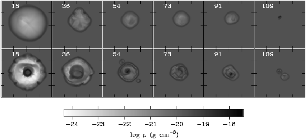
Figure 2: Axial cross sections of density from Run D (upper row) and from Run I (lower row). Each row is from the time displayed in the corresponding panel in Figure 1. Each cross section is scaled to the same maximum and minimum and the scale, with darker shading to indicate denser regions, is displayed below the cross sections. We display the complete computational domain in the two axes shown. The distance between adjacent tick marks is 5 $\times$ 10¹⁵ cm. The axial position in R_j is given in the upper left of each panel. The vertical axis is the $y$-axis, and the horizontal axis is the $z$-axis, and so the view is from the jet inlet boundary looking down the jet axis (i.e., toward the +$x$-direction).

In Simulation I, we wish to show the consequences of increasing the mass density in a light jet flow that had already propagated some distance. In this case, the density evolution follows a less abrupt change, determined by the following:

$$\rho_{j}(t)=\rho_{0}+\rho_{1}\tanh\Big{(}\frac{t-t_{1}}{t_{0}}\Big{)}$$ (1)

where we set $\rho_{1}$ = 1.1484 $\times$ 10^-19 g cm^-3, $\rho_{0}$ = 1.1716 $\times$ 10^-19 g cm^-3, $t_{1}$ = 800 years, and $t_{0}$ = 50 years. This results in the logarithm of the jet hydrogenic number density rising from $\log n_{j}$ = 3 to $\log n_{j}$ = 5 over a 200 year period centered at a program time 800 years after the simulation has started. Given the axial grid length of 2 $\times$ 10¹⁷ cm, this leads to the bow shock from the initially light jet being roughly half way across the grid when the mass flux is increased.

3 Internal Structure

Slices of jet density down the midplane are presented in Figure 1. Both simulations feature a refocused leading region and wider trailing “shoulders”. We remark that the shoulder regions in both simulations shown in Fig. 1 have progressed to only 7 $\times$ 10¹⁶ cm, a small fraction of the jet length. In our study of non-evolving jets (Rosen & Smith, 2003), we were able to attribute the refocusing to the combination of both shear and strong molecular cooling, since simulations with atomic jets or molecular jets with no shear do not refocus. The ratio of the distance of the shoulders from the nozzle relative to that of the entire jet was found to be proportional to the jet-to-ambient density ratio. Hence, without a continuous strong power source in Simulation D, the bloated cocoon is stunted.

Furthermore, the average speed of the leading bow shock, which almost traverses the grid in 1300–1400 years, is $\sim$ 45 km s^-1. This is similar to a “light” jet simulation (jet-to-ambient density ratio of 0.1 in Rosen & Smith 2003). This average speed is still, however, nearly 90% faster than expected from ram pressure arguments due to the concentration of the jet thrust caused by the refocusing.

From a plot of a time-averaged advance speed of the bow shock (Figure 3), we see that the advance speed of the bow shock is not constant throughout either simulation. In Run D, the advance speed of the jet falls below 60 km s^-1 within the first 100 years, and follows a linear decrease in velocity with time until t $\sim$ 800 years, where it continues a linear decrease but at a faster rate. The change of the deceleration rate is related to a broadening of the tip of the bow shock, which is at the leading edge of a region of refocused and accelerated flow after $t\sim$ 200 years. At the end of Simulation D the bow shock is progressing at a speed of $\sim$ 30 km s^-1. This is an example of the ability of all of our aborted molecular jet simulations to maintain its momentum for the length of the computational grid (0.06 pc). Even in the case of the jet aborted after 5 years, we still found a speed of $\sim$ 20–25 km s^-1 after the 2000 year interval in which it crossed the grid.

Figure 3: Time-averaged advance speed of the bow shock. The advance speed here is determined from the leading edge of the bow shock in integrations of H₂ emission, similar to Figures 4 and 5.

In contrast, the progress of the bow shock in Simulation I, as measured from the molecular emission maps presented below, increases early in the simulation. The speed initially drops to 20 km s^-1, but after only 50 years begins to rise. There is a significant increase at $t\sim$ 300 years, after which the speed of advance of the bow shock is $\sim$ 50 km s^-1. The increase does not coincide with the onset of the higher jet density but, instead, coincides with the initial refocusing of the bow shock at its leading edge. Thus, the stripping of the low-speed jet sheath is an interesting means by which an acceleration in the proper motions of jet knots may result. Even after the jet density has increased, the average advance speed for the bow shock remains nearly constant until the simulation is terminated.

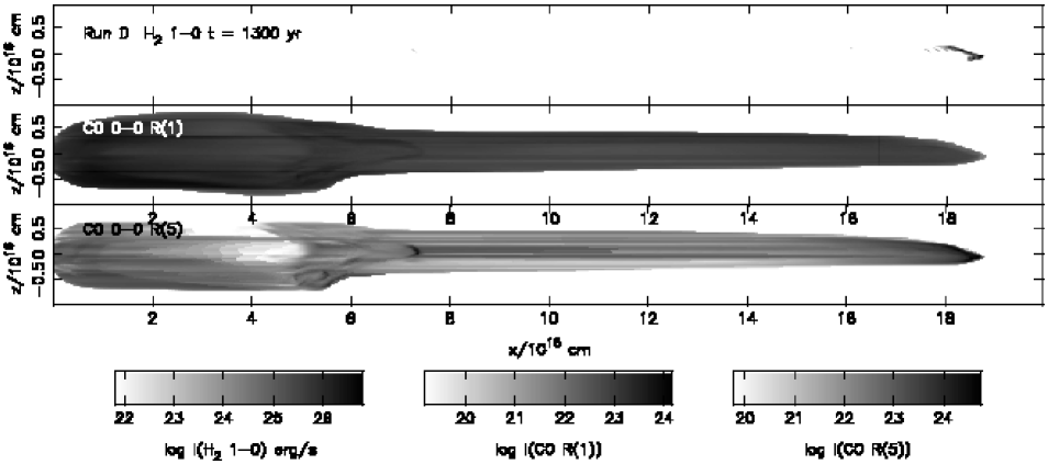
Figure 4: Appearance of Simulation D in three molecular emission lines. The luminosities from each zone are placed in bins in the viewing window that are the same size as the 3D zones used in the simulations (i.e., 2 $\times$ 10¹⁴ cm). The axis being integrated is the $z$-axis, so the vertical axis in all the panels is the $y$-axis.

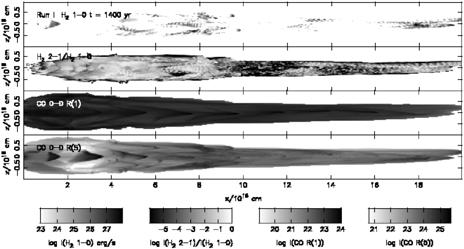
Figure 5: Appearance of Simulation I in four molecular emission lines. See caption in Fig. 4. Since this simulation generated sufficient amounts of warm (T $\sim$ 10,000 K) gas, we show the map of the H₂ 2–1 S(1) emission in the second panel.

The dense material in Simulation D is confined to the bow shock and swept-up shell while dense material is also associated with the internal shocks of the pulsed jet in Simulation I. The cocoon surrounding the jet behind the shoulder region has the lowest density, with the still-connected jet in Simulation I having a lower minimum density by a couple of orders of magnitude than the aborted jet in Run D. These overdense and underdense regions within the jet are also apparent in the axial cross sections of density in Figure 2. With the ability of the jet in Run I to generate a very low density cocoon, the relatively small overdensity (still an order of magnitude) in the bow shock is difficult to see. Note twin concentric shell structures are formed in the cross section of Run I, visible in Fig. 2 at distances R_j = 54–91, where the powerful jet transmits invigorated shocks through the cocoon.

4 Simulated Molecular Line Emission

4.1 The Spatial Distributions

Images of line emission from molecules are shown for Simulation D in Fig. 4 and for Simulation I in Fig. 5. Integration is across the $y$-direction transverse to the jet axis, and the simulation time corresponds to the previous figures. The H₂ line emission is based on a non-LTE approximation to the vibrational populations (Hollenbach & McKee, 1979), and the CO emission is calculated from the formulae of McKee et al. (1982). In addition, we set a lower velocity limit of 1 km s^-1 on the integration of CO emission lines in order to subtract out the undisturbed cloud.

In Figure 4, we show the H₂ 1–0 S(1) line, the CO R(1) and R(5) lines for the CO ground vibrational state ($\upsilon$ = 0). In the H₂ line, only the leading edge of the bow shock remains visible and, since Simulation D is relatively devoid of warm (T $>$ 5000 K) gas, the image in the H₂ 2–1 S(1) line is not shown. We display instead the CO R(5) line, which should highlight gas at intermediate temperatures (T $\sim$ 100 K) between the H₂ line and the CO R(1) line (which emphasizes the coldest, T $\sim$ 5 K gas). The CO R(5) line image not only has an intermediate appearance but also shows some filamentary structure, which is brightest at the leading edge of both the bow shock and the shoulders. This relatively warm gas is generated by the accelerating refocused region. In both of the simulations presented here, the moving CO R(1) shows the outline of the bow shock.

Figure 6: Integrated molecular emission in three lines for each simulation. The H₂ 1–0 emission is the solid line, the H₂ 2–1 is the dotted line, and the CO emission is the dashed line.

Simulation I is sufficiently energetic to generate copious amounts of 10,000 K gas. Hence, in addition to the lines shown in Fig. 4, we also show the relative luminosity of the H₂ 2–1 line to the 1–0 line in Fig. 5. The emission in the H₂ 1–0 image is sparse and filamentary, showing several ‘minibows’ especially at the edges of the shoulder region near $x=$ 9 $\times$ 10¹⁶ cm. Only a single pulse near the inlet is seen in the H₂ 1–0 map. Earlier pulses, farther down the jet, are easier to see in the ratio of the H₂ lines, and are noticeable in the CO R(1) line, but very prominent in the map for the CO R(5) line. While the CO R(1) emission map does show a wider shoulder region well behind the leading edge of the bow, this region is much less pronounced than the appearance in the midplane density slice.

4.2 Totals

The evolution of the totals of the H₂ emission lines and the CO R(1) line are shown in Fig. 6. In Simulation D, a dramatic reduction in the H₂ totals begins after $t$ = 100 yr. A flattening of the CO luminosity, which monotonically increases for non-evolving molecular jets, also occurs but not until $t$ = 700 yr. Thus, a significant change in the ratio of the H₂/CO total emission occurs shortly after the flow has been turned off. It is only when the H₂ 1–0/CO R(1) ratio approaches unity that the total emission from each emission line tends to flatten out. Before this occurs the ratio is a good age indicator for the aborted jet flow.

The 80 year delay between the jet demise and the H₂ weakening is clearly the time to elapse before the leading bow stops being driven by the jet impact. The 700 year delay between the termination of the jet flow and the flattening of CO R(1) emission indicates that new ambient material continues to be snowploughed, as the momentum of a small fraction of high-speed gas is redistributed into a large fraction of low-speed gas. This is a true ‘bullet’ or ballistic phase. To test this, the deceleration of the bow shock in Run D as shown in Fig. 3 can be compared to the analytic motion of a bullet of speed $v_{b}$, fixed mass M, cross-sectional area A, and initial density $\rho_{bo}$, moving into a medium of density $\rho_{a}$, with a drag coefficient D_c. The equation of motion is

$$\frac{d\,v_{b}}{d\,t}=-\frac{v_{b}^{2}}{L}$$ (2)

where $L=M/({\rm D}_{c}\rho_{a}A)$. Here L defines an effective column length of ambient gas required to slow down the bullet. First, we take ram pressure confinement of a bullet which maintains its shape as the pressure decreases. This yields

$$L=L_{o}\left[\frac{\rho_{bo}}{\rho_{a}}\right]^{2/3}\left[\frac{v_{b}}{c_{s}}\right]^{4/3},$$ (3)

where $c_{s}$ is the bullet sound speed and $L_{o}$ is the initial value of L. Substitution and integration gives

$$t=3\frac{L_{o}}{v_{bo}}\left[1-\left(\frac{v_{b}}{v_{bo}}\right)^{1/3}\right]$$ (4)

and

$$x=\frac{3}{4}\,L_{o}\left[1-\left(\frac{v_{b}}{v_{bo}}\right)^{4/3}\right].$$ (5)

Alternatively, if the bullet is either disk shaped or does not expand at all, L is a constant and we find

$$\frac{v_{b}}{v_{bo}}=\frac{1}{1+t\,(v_{bo}/L)}.$$ (6)

For the particular conditions of Run D, $L_{o}=(6\times 10^{16}/D_{c})$ cm. To decelerate from 60 km s^-1 to 30 km s^-1 in 1200 yr, then requires D_c = 0.17–0.28, depending on the bullet model utilised. This drag coefficient is then consistent with the aerodynamic shape of the leading bow and thus shows that a large mass can be mildly disturbed by a high-speed jet.

The duration of this phase is 35 times longer than the jet-driving phase, suggesting an effective jet column density which exceeds the deflected ambient column density by 35. We can roughly attribute this to the high jet density (10) and the refocusing (3.5).

It should be remarked that decelerating bullets have been investigated in various astrophysical contexts including Herbig Haro objects (Norman & Silk, 1979), radio galaxies (Smith & Norman, 1980) and planetary nebula (Palmer et al., 1996). Depending on how the bullet forms, stability is maintained through inertial confinement for a sound-crossing time or a shock-wave crossing time. Therefore, the high Mach number of the bullet in Run D permits a bullet to travel over 10¹⁷ cm without great expansion.

In Run I, periodic brightening in H₂ luminosity occurs as the pulses in the flow pass through the shoulder region and energise the bow shock envelope. The increase in jet density that becomes significant for $t>$ 750 yr shows up as an increase in the H₂ output very soon thereafter ($t$ = 800 yr). No accompanying increase in the CO emission is noticeable. There is an unrelated early break in the rate of increase in the CO R(1) total luminosity, at t = 100 yr. The slightly increased rate is related to the shape of the envelope, which shows the effects of refocusing near the start of the simulation.

The final integrated fluxes of the two simulations have contrasting behaviours. In Run D, the absolute luminosity in the 1–0 S(1) line of H₂ is continued at the low level of L(1–0 S(1)) $\sim$ 10^-5 L_⊙ despite the lack of a jet. This compares to the value of $\sim~{}10^{-3}$ L_⊙ for the equivalent simulation in which the jet power is maintained (Rosen & Smith, 2003). In Run I, L(1–0 S(1)) reaches 3 $\sim~{}10^{-4}$ L_⊙ and is set to increase. It is clear that a complex relationship exists between the immediate jet power and L(1–0 S(1)). Whereas we found this ratio to lie in the range 80–600 for non-evolving jets (Rosen & Smith, 2003), we here find values between zero (Run D, after 20 yr) and 1.2 $\times$ 10⁵ (Run I, 800 yr).

The predicted values of L(1–0 S(1)) are comparable to those derived in the unbiased statistical study of (Stanke et al., 2002), where the majority of outflows possess L(1–0 S(1)) in the range 10^-4–10^-3 L_⊙. Nevertheless, the absolute fluxes are quite low in comparison to a number of observations of well-known outflows. This is partly due to the compactness of the simulated outflows, limited by our need to follow molecule dissociation. We can argue that scaling up the spatial dimensions by a factor of 10 would scale the luminosities by a factor of 100. It remains to be shown, however, that the flow patterns would be maintained.

5 Velocity Distribution of Mass and Molecular Line Emission

Table 1: Mass Spectra Power-Law Dependences

Sim.	t(yr)	type	$\theta$	range of log v	$\gamma$	Na	type	$\theta$	range of log v	$\gamma$	Na
D	1300	mass	15	0.5–1.0	1.19	7	CO	15	0.2–0.6/0.7–0.9	1.27/1.92	2/3
			30	0.5–1.0	1.17	7		30	0.5–1.0/0.9–1.1	1.17/2.74	7/5
			45	0.5–1.0	1.19	7		45	0.5–1.0/1.1–1.2	1.22/3.58	7/3
			60	0.5–1.0	1.10	7		60	0.5–1.0/1.1–1.3	1.16/3.07	7/7
			90	0.5–1.0	1.13	7		90	0.5–1.0/1.2–1.3	1.21/3.18	7/7
I	1300	mass	15	0.5–1.0	1.05	7	CO	15	0.5–1.0	1.20	7
			30	0.5–1.0	1.01	7		30	0.5–1.0	1.22	7
			45	0.5–1.0	0.99	7		45	0.5–1.0	1.22	7
			60	0.5–1.0	1.01	7		60	0.5–1.0	1.21	7
			90	0.5–1.0	1.03	7		90	0.5–1.0	1.21	7

• N is the number of points in the velocity distribution, which was computed in 1 km s^-1 bins, used to estimate the slope.

5.1 Mass “Spectra”

CO velocity data for observed outflows are now invariably analysed by plotting the differential mass in velocity bins, with a few simple assumptions made to compute mass from CO intensity. One may classify how this mass decreases with velocity by fitting a power law, with the slope defined by $dm/dv\propto v^{-\gamma}$. Two surveys containing many sources (Yu et al. 2000 and Ridge & Moore 2001) conclude that a broken power law is often necessary, with a shallow slope of 1.0–2.0 at low velocities and a steeper slope, in some cases $\gamma$ is close to 10, at larger velocities. The velocity where the break occurs is usually $\sim$ 10 km s^-1. One interpretation of this break speed is that it is the projected component of the critical shock speed, $v_{d}\cos\theta$ with $v_{d}$ = 23 km s^-2 (e.g., Smith 1994), above which all molecules are assumed to dissociate within the shock.

We have performed a similar analysis for the velocity distributions of mass, of CO R(1) luminosity and of H₂ 1–0 luminosity for each of the aborted jet simulations, including Simulation D, and for Simulation I. In the case of Simulation D, the analysis was performed at a program time of $t$ = 1300 yr, corresponding to other Simulation D illustrations presented here. In the increased-density jet of Simulation I, the tip of the jet has just barely reached the outer $x$-boundary at $t$ = 1400 yr. We, therefore, chose to inspect data at $t$ = 1300 yr. We list the results for a sample of viewing angles, defined as the angle of the jet axis out of the plane of the sky and toward the observer, in Table 1. We display the data for one viewing angle (15^∘) in Figure 7.

Having only found low values of $\gamma$ in previous simulations involving molecular jets (although high values are possible for an atomic jet), we have chosen to investigate whether a reduced mass flux would give larger values for $\gamma$. In Simulation D and the other aborted jet simulations, however, we still find shallow dependences of the mass distribution on velocity i.e. small values for $\gamma$. The values for the aborted jet simulations are in general larger than their counterparts in the increasing jet-density simulation, with the values for both sets usually nearer 1.0 than 2.0. However, large slopes are computed for high velocities in the only cases where a break could be seen, which are the CO-derived values for the aborted jet simulation. These results are not significantly different than those found for non-evolving jets (Rosen & Smith, 2003).

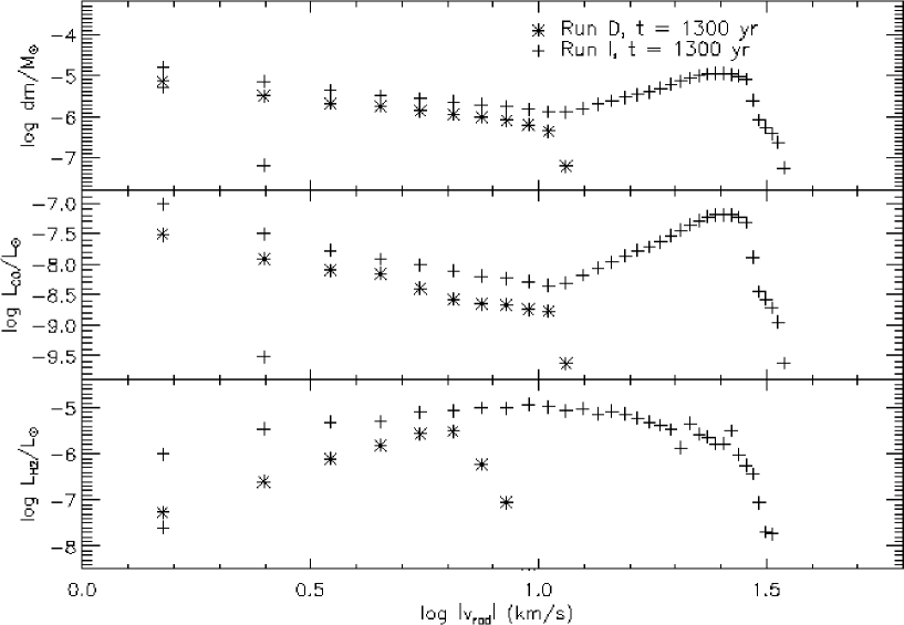
Figure 7: Distribution of velocities into bins of mass and two molecular line luminosities for a viewing angle of 15^∘. Displayed are the distribution of mass (top panel), CO luminosity (middle panel) and H₂ 1–0 emission (lower panel). Each velocity bin is 1 km s^-1 wide. The designation for the data presented in each panel is shown in the top panel. Each run may be represented twice within each panel, with data from both positive and negative radial velocities included. Naturally, the smaller ranged data is for the positive radial velocities (which could contribute to a “red” lobe, while the other is from a “blue” lobe).

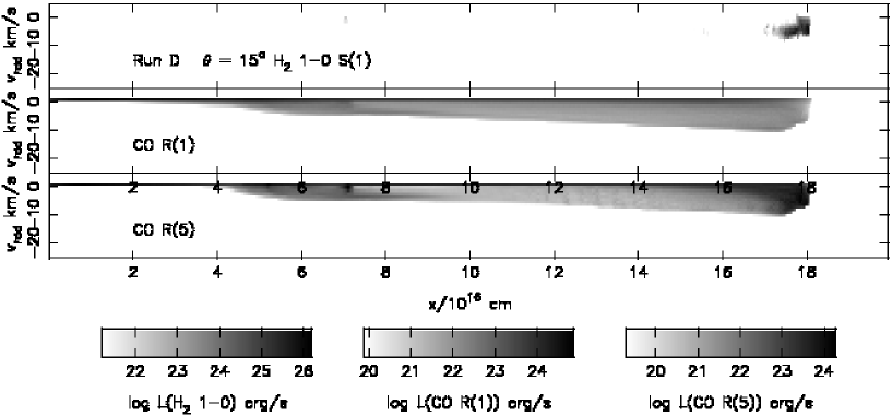
Figure 8: Position-velocity map for Run D in three molecular emission lines. The jet axis is 15^∘ out of the plane of the sky toward the observer. Each bin spans 2 $\times$ 10¹⁴ cm in $x^{\prime}$, the jet axis projected on the plane of the sky, and 1 km s^-1 in radial velocity.

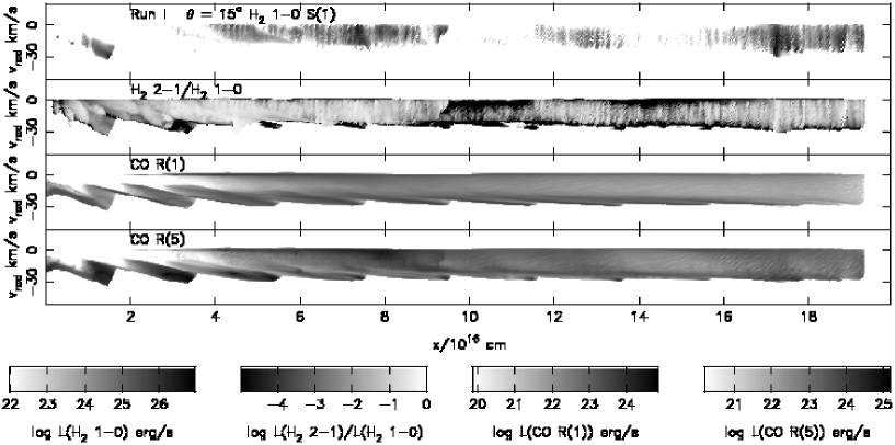
Figure 9: Position velocity map for Run I in four molecular emission lines. The jet axis is 15^∘ out of plane of the sky toward the observer. Each bin spans 2 $\times$ 10¹⁴ cm in $x^{\prime}$, the jet axis projected on the plane of the sky, and 1 km s^-1 in radial velocity.

In the previous analysis for non-evolving molecular jets, the $\gamma$ determined for CO was nearly uniformly larger than that for mass. For the evolving jet simulations here, the dependence of CO luminosity on velocity is also usually steeper than the one for mass, but in some cases it is only equal (e.g., Run D at a viewing angle of 30^∘) or, for one aborted jet simulation, was lower. This occurred in a simulation of an aborted jet that propagated into an equal pressure ambient medium. The CO-derived $\gamma$ is lower than the mass-derived one at all viewing angles, and by as much as 0.6. However, in this simulation, the CO distribution can be better fitted with two power laws, with the higher velocity one much higher than the single linear fit to the mass distribution.

Very little dependence of $\gamma$ on viewing angle is found for both of these simulation. This is contrary to previous jet simulations (Smith et al. 1997, Lee et al. 2001, Downes & Cabrit 2003, and Rosen & Smith 2003), which have shown an inverse relationship between viewing angle and $\gamma$. However, the CO-derived slopes in the high velocity range are again an exception. This group disagrees more strongly with the previous results and, for small viewing angles, $\gamma$ varies in direct proportion to the viewing angle.

An excess at the highest velocities is found in Simulation I, as also found in previous studies of non-evolving molecular jets. This bump peaks at log $v$/km s^-1 = 1.4 (for a viewing angle of 15^∘) and is associated with the internal shocks from the pulsed jet. In the aborted jet simulations, both the internal shocks and the high velocity bump are absent.

Recent observations of H₂ emission from protostellar outflows have been similarly analysed (Salas & Cruz-González, 2002). As with the CO data, the H₂ flux distributions show a break in behaviour, with the break between 2–17 km s^-1 for the selection of sources. A flat or slightly rising flux is found at low velocities and a fall-off in flux with $\gamma$ in the range between 1.8 and 2.6 at high velocities.

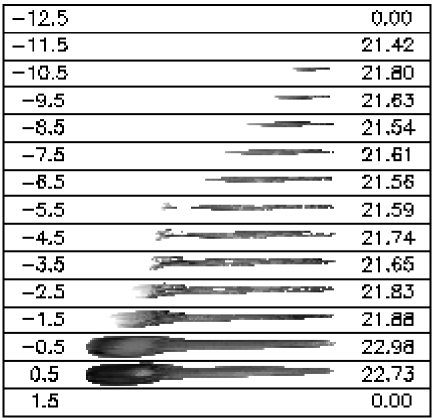
Figure 10: Velocity channel map for Simulation D in CO R(1) emission. The jet is viewed 15^∘ out of the plane of the sky toward the observer. The central radial velocity in km s^-1 is indicated on the left side of each panel. Four orders of magnitude in luminosity are displayed in each panel. The log of the maximum luminosity in ergs s^-1 is shown on the right side of each panel. Each bin spans 2 $\times$ 10¹⁴ cm in $x^{\prime}$, the jet axis projected onto the plane of the sky, and in $y$.

From Fig. 7, we see that Run I may best match these observational constraints. However, the H₂ flux distribution in Run I rises one order of magnitude in brightness from the first H₂ datum in the figure to where it turns over near $v$ = 10 km s^-1. This is much larger than that found in the observations, although it is a smaller rise than found in the non-evolving molecular jets simulations. Additionally, the best fit line between $\log v$ = 1.0 and 1.3 has $\gamma$ = -1.6, which is in line with the observations. This could be an adequate explanation for sources viewed with their jet axis near the plane of the sky, such as HH 212. However, at larger viewing angles (Fig. 7 shows a viewing angle of 15^∘ only), the low-velocity rise steepens. In addition, at intermediate velocities the comparison becomes less good as the viewing angle is increased. C-type shock physics may solve these problems since ambipolar diffusion would generate considerably more emission near zero radial velocity in the absence of discontinuous acceleration. The effect this has on the global properties of an outflow remain to be calculated.

5.2 Position-Velocity Maps

We display position-velocity maps in H₂ and CO emission lines for Simulation D (Fig. 8) and Simulation I (Fig. 9). The H₂ 1–0 position-velocity map for Simulation D shows emission only at the leading edge of the jet. This emission is spread over 10 km s^-1 and 1 $\times$ 10¹⁶ cm along the projected jet axis and is characterised by two peaks. Note that steady state bow shock models (see Fig. 14b of Smith et al. 2003) predict two peaks, which correspond to (1) the projected edge-on leading edge near zero radial velocity and (2) the blue-shifted emission from the warm material projected well behind the bow apex.

The pulsed jet in Simulation I shows intermittent H₂ 1–0 and 2–1 emission along its length, with many emission sites spreading out over a large range of velocities. The H₂ 2–1 map shows that the sites of bright H₂ 1–0 emission are also bright in the more highly excited line.

The emission in the CO lines shows a pair of “Hubble-law” like dependences for Simulation D, but disconnected from the nozzle. The outer envelope of the first increases relatively quickly with position, and is followed by a shallower increase for much of the remainder of the jet. While the emission in the CO R(1) line is nearly uniform for non-zero velocities, there is some structure in the CO R(5) position-velocity diagram. The bright spot near $x^{\prime}$ = 7 $\times$ 10¹⁶ cm is from the advancing edge of the shoulder region seen in Fig. 4, and the peak at $x^{\prime}$ = 5 $\times$ 10¹⁶ cm is from the trailing filamentary structure. Both of these bright features have radial speeds near zero.

For Simulation I, the CO R(5) diagram shows more structure than the diagram for CO R(1). Both show a prominent series of triangular shapes that distinguish the Hubble Law behaviour of a pulsed jet. There is evidence for a connective loop of emission between successive Hubble Law regions, until the triangles merge downstream, filling in all velocities, and the Hubble Law is then hidden. The maximum luminosity in the CO R(5) map falls in between those of the H₂ 1–0 and the CO R(1) maps. Naturally, all of the maxima are higher than the corresponding values in the aborted jet simulation.

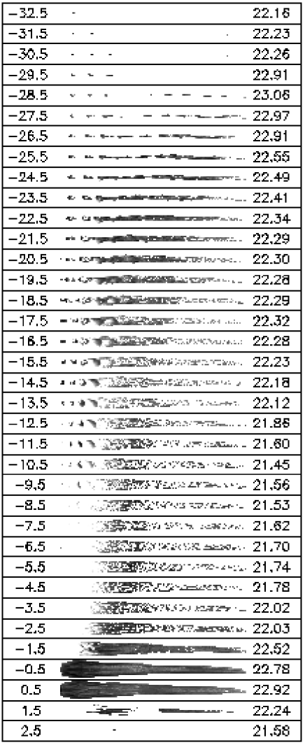
Figure 11: Velocity channel map for Simulation I in CO R(1) emission. The jet is viewed 15^∘ out of the plane of the sky toward the observer. The central radial velocity in km s^-1 is indicated on the left side of each panel. Four orders of magnitude in luminosity are displayed in each panel. The log of the maximum luminosity in ergs s^-1 is shown on the right side of each panel. Each bin spans 2 $\times$ 10¹⁴ cm in $x^{\prime}$, the jet axis projected onto the plane of the sky, and in $y$.

5.3 Velocity Channel Maps

We display CO R(1) velocity channel maps for Simulation D in Fig. 10 and Simulation I in Fig. 11 with a resolution of 1 km s^-1. While the CO emission from Simulation D does not span a large velocity range, the morphology does change as one moves from relatively high radial velocity (10 km s^-1) to low radial velocity. At high radial velocities, only the leading edge of material is visible, and as the velocity is decreased more emission appears closer to the inlet. This is another aspect of the Hubble Law profile seen in the position-velocity map. Near zero velocity the entire envelope of the jet and cocoon of shock ambient material is represented, along with the shoulder region seen in the density cross sections and integrated CO maps. This defines a T-type morphology. Even the filamentary structure seen in the integrated emission map for CO R(5) is seen to some extent in these CO R(1) velocity channel maps.

The CO R(1) velocity channel maps for Simulation I reveal morphologies in the different velocity ranges more typical of our previous non-evolving jets (Rosen & Smith, 2003). At high radial velocities, only the internal shocks from the pulsed jet are seen and at low velocities the entire envelope of jet plus cocoon material is present. At low velocities, the gap between the nozzle and the onset of emission decreases and a V-type global morphology is identifiable. At intermediate velocities, a spinal structure is present.

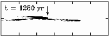
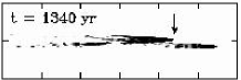
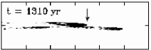
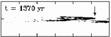
Figure 12: Birfucating bow shocks shown in the H₂ 1–0 line for Simulation I. We display the portion of the computational grid with $x$ = 1.4–2.0 $\times$ 10¹⁷ cm. Adjacent tick marks are 1 $\times$ 10¹⁶ cm apart. An arrow points out the progress of the bow shock associated with the denser flow.

The twin protuberances at the front of the jet are from the differing advance speeds associated with the extrema of the evolving jet density in Simulation I. As confirmed from a sequence of integrated H₂ 1–0 emission line maps (Fig. 12), a faster-moving bow shock leaves the path of the earlier slower-moving initial bow shock. This departure occurs at a fairly late time in the evolution of the jet ($t$ = 1300 yr, or 550 yr after the onset of the increase in jet density at the inlet) and well into the refocused leading part of the bow ($x$ = 1.6 $\times$ 10¹⁷ cm). The average speed of the new bow is therefore close to 100 km s^-1. An average speed for the propagation of the new bow shock equal to that of the (time-averaged) jet speed is not unreasonable in this simulation with the very light initial jet initially evacuating the path and with an acceleration from the refocused region.

6 Application: an evolutionary diagnostic?

The structures and features detailed above can provide clues to distinguish the evolutionary phase of a specific outflow. Statistically, however, the integrated properties can provide the most employable measures. In particular, the ratio L(H₂ 1–0 S(1))/L(CO R(1)) can be determined from simulations and compared to the observationally derived L(H₂)/L_mech. The total molecular hydrogen emission L(H₂) can be estimated from L(H₂ 1–0 S(1)) (Smith, 1995), provided the near-infrared extinction can be determined. The mechanical luminosity for both lobes in a bipolar outflow is derived from formulae of the form L_mech = M_co $v_{co}^{3}$/(2 $l$) where M_co is derived from L(CO R(1)), assuming a CO abundance and temperature, $v_{co}$ represents the appropriately averaged speed of the mass that dominates the outflow energy (and must account for the source orientation when derived) and $l$ is the outflow size.

From the ratio of mass to L_co in the log $v$ bins of Figure 7, we estimate from the simulations that M_CO for one side of a bipolar outflow $\sim$ 300 L(CO R(1)) in solar units. Furthermore, given the consistently low values of $\gamma$, we take $v_{co}$ = 20 km s^-1. Finally, we fix L(H₂ 1–0 S(1)/L(H₂) = 0.05. It must be remarked that a rather high number of assumptions precede a comparison of simulation and observation. Nevertheless, it is clear that the ratio L(H₂ 1–0 S(1))/L(CO R(1)) $\sim$ 3–8 for Run D after 1000 yr, while L(H₂ 1–0 S(1))/L(CO R(1)) $\sim$ 30–40 for Run I after 1000 yr. Given the above factors these convert to: L(H₂)/L_mech $\sim$ 0.02–0.05 for Run D and $\sim$ 0.2–0.3 for Run I.

We confirm that strong H₂ flows are thus associated with Run I. For example, we find L(H₂)/L_mech $\sim$ 0.3 for Cepheus E, one of the dynamically youngest outflows (Smith et al., 2003). Moreover, the H₂ emission is widespread and the CO position-velocity diagram displays structure cutting through all radial velocities at all positions, rather than the triangular Hubble-law features (Ladd & Hodapp, 1997), consistent with the Run I predictions. Finally, we note that the CO $\gamma$ values for Cepheus E are 0.99 and 1.8, for the two lobes, although these values are quite sensitive to the chosen local standard of rest (Smith et al., 1997). Hence, observations of Cepheus E are consistent with our results for a newly-forming outflow.

To date, CO emission has not been fully resolved in many outflows. Velocity channel maps are thus rare. A highly collimated CO outflow emanates from IRAS 21391+5802, with a V-shaped morphology on velocity channel images (Beltrán et al., 2002). The V-shape suggests that it is also an immature outflow in which the central source is increasing in power. We would thus expect to find a strong H₂ outflow, as is, indeed, the case: the total shocked emission is estimated to be 4 L_⊙ whereas the mechanical power estimates lie in the range 0.15–1.2 L_⊙ (Nisini et al., 2001).

In contrast, there are many examples of outflows with very weak total H₂ emission. These include the HH 366/B5 IRS1 outflow in the Perseus cloud complex, which possesses high collimation. Hubble-law behaviour, consistent with a single outburst in the past is also present (Yu et al., 1999). The H outflow in OMC-2 is another example, where the presently-observed H₂ jet does not appear to be the driver for the CO outflow (Yu et al., 2000).

IRAS 18148-0440 in the L483 core is thought to be a protostar undergoing the transition from Class 0 to Class 1. Its CO outflow may possess a T-shaped morphology, although background cloud subtraction makes this uncertain (Tafalla et al., 2000). It belongs to a class of objects characterised by low velocity CO and no CO bullets, as also predicted here for a transitional outflow (Tafalla et al., 2000).

7 Summary

We have reported on two jet simulations that model drastic jet density evolution over tens or hundreds of years. The basic physical structure is similar to that previously found for non-evolving sheared molecular jets (Rosen & Smith, 2003), with an accelerated leading bow shock followed by a wider, slower shoulder-like region. More specifically, both of the simulations on display here resemble a light molecular jet simulation. The primary reason for this is that the shoulder region makes only slow progress relative to the leading edge of the bow shock.

We have explored predicted features relevant to high resolution near-infrared (H₂ rovibrational at 2.12$\mu$m emission), far-infrared (CO R(5) rotational emission at 435$\mu$m) and millimetre (CO R(1) rotational emission at 1.3mm) wavelength observations. As expected, the H₂ lines reveal patchy details of the structure and the CO lines show the general outline of material encompassed by the bow. CO line emission from mid-level rotational states show both the general outline and the internal shock structure. Owing to the small amount of higher temperature gas in the aborted jet simulation, the H₂ emission is limited to the very tip of the accelerated bow shock. The predicted values of the 1–0 S(1) 2.12$\mu$m luminosity are comparable to those derived for the majority of outflows in the unbiased statistical study of Stanke et al. (2002).

The evolution in the integrated luminosity in these molecular lines is evident in both simulations. The changes in the integrated values of H₂ occur at program times that are within 100 yr after the modification of the inflow jet density. Of particular note is the ratio of the integrated H₂ to the integrated CO R(1) line in the aborted jet case, which decreases dramatically with time. Thus, in principle this ratio can be used to estimate the age of an outburst or aborted molecular flow from a protostellar core.

We have also computed velocity distributions in mass, CO luminosity, and H₂ luminosity. Here the main results are:

1. The slopes of these distributions are small, closer to one than two in most cases. Steeper slopes ($\gamma$ = 2–3) are seen at high velocities in CO in the aborted jet simulation.

2. The slopes for the aborted jet case are larger than those for the increasing jet density case, although not by a large amount for the simulations listed in Table 1.

3. Similar to non-evolving jets (Rosen & Smith, 2003), $\gamma_{\rm CO}$ is usually greater than $\gamma_{\rm mass}$, but there are significant exceptions.

4. In the aborted jet simulation, there is no excess in the amount of mass or CO at the highest velocities; we have seen this excess that is associated with the internal shocks of a pulsed jet.

The position-velocity maps for the aborted jet case are relatively featureless. In CO emission, a triangular Hubble-Law outline is filled in by the emission but does not include the low velocity emission near the jet inflow boundary. The CO R(5) position-velocity map shows some fine structure, with brighter regions associated with the warmer parts of the flow: the leading part of the bow shock and some internal structure near the front of the shoulder region.

In the increasing jet density simulation, the position-velocity CO maps show the series of Hubble Law regions associated with successive pulses in the jet. Additionally, the CO R(5) map has more structure than the CO R(1) map. In the H₂ position-velocity map, there are numerous features that are narrow along the jet axis but cover a large range of velocities (the vertical lines in Fig. 9).

The CO R(1) velocity channel maps for the aborted jet simulation have emission confined to a small range of velocities. The sequence of channel images shows a T-morphology at low velocities and the characteristics typical of a Hubble Law at high velocities. The channel maps for the increasing jet density simulation possess a V-morphology, with the inclusion of an additional protuberance from the new denser flow that carves a fresh path near the previous flow.

These features, combined with the levels of integrated emissions, suggest that jets in certain outflows (e.g. IRAS 21391+5802 and Cepheus E, see Sect. 6) are increasing in power, while other jets (e.g. that from IRAS 18148-0440 in L483) are on the decline.

Not many detailed velocity channel maps have as yet reached the literature. This will change shortly, and with the advent of new telescopes such as SIRTF, FIRST and ALMA, imaging and spectroscopy will reveal the properties on fine scales in many molecular lines of intermediate and low excitation, such as in the CO R(5) and R(1) lines. Here we have determined how these properties can help determine the jet evolutionary stage.

References

- Andre et al. (1993) Andre P., Ward-Thompson D., Barsony M., 1993, ApJ, 406, 122
- Arce & Goodman (2001) Arce H. . G., Goodman A. A., 2001, ApJ, 551, L171
- Beltrán et al. (2002) Beltrán M. T., Girart J. ., Estalella R., Ho P. T. P., Palau A., 2002, ApJ, 573, 246
- Cabrit & Raga (2000) Cabrit S., Raga A., 2000, A&A, 354, 667
- Chandler & Richer (2001) Chandler C. J., Richer J. S., 2001, ApJ, 555, 139
- Davis et al. (1998) Davis C. J., Smith M. D., Moriarty-Schieven G. H., 1998, MNRAS, 299, 825
- Downes & Cabrit (2003) Downes T. P., Cabrit S., 2003, A&A, in press
- Falle (2002) Falle S. A. E. G., 2002, ApJ, 577, L123
- Fridlund & Liseau (1998) Fridlund C. V. M., Liseau R., 1998, ApJ, 499, L75
- Gueth & Guilloteau (1999) Gueth F., Guilloteau S., 1999, A&A, 343, 571
- Gueth et al. (2001) Gueth F., Schilke P., McCaughrean M. J., 2001, A&A, 375, 1018
- Hartigan et al. (2001) Hartigan P., Morse J. A., Reipurth B., Heathcote S., Bally J., 2001, ApJ, 559, L157
- Hollenbach & McKee (1979) Hollenbach D., McKee C. F., 1979, ApJS, 41, 555
- Lada (1987) Lada C. J., 1987, in IAU Symp. 115: Star Forming Regions Vol. 115, Star formation - From OB associations to protostars. pp 1–15
- Ladd & Hodapp (1997) Ladd E. F., Hodapp K.-W., 1997, ApJ, 474, 749
- Lee et al. (2000) Lee C., Mundy L. G., Reipurth B., Ostriker E. C., Stone J. M., 2000, ApJ, 542, 925
- Lee et al. (2001) Lee C., Stone J. M., Ostriker E. C., Mundy L. G., 2001, ApJ, 557, 429
- Lim et al. (2002) Lim A. J., Raga A. C., Rawlings J. M. C., Williams D. A., 2002, MNRAS, 335, 817
- McKee et al. (1982) McKee C. F., Storey J. W. V., Watson D. M., Green S., 1982, ApJ, 259, 647
- Nagar et al. (1997) Nagar N. M., Vogel S. N., Stone J. M., Ostriker E. C., 1997, ApJ, 482, L195
- Narayanan & Walker (1996) Narayanan G., Walker C. K., 1996, ApJ, 466, 844
- Nisini et al. (2001) Nisini B., Massi F., Vitali F., Giannini T., Lorenzetti D., Di Paola A., Codella C., D’Alessio F., Speziali R., 2001, A&A, 376, 553
- Norman & Silk (1979) Norman C., Silk J., 1979, ApJ, 228, 197
- Palmer et al. (1996) Palmer J. W., Lopez J. A., Meaburn J., Lloyd H. M., 1996, A&A, 307, 225
- Ridge & Moore (2001) Ridge N. A., Moore T. J. T., 2001, A&A, 378, 495
- Rosen & Smith (2003) Rosen A., Smith M. D., 2003, A&A, submitted
- Salas & Cruz-González (2002) Salas L., Cruz-González I., 2002, ApJ, 572, 227
- Smith (1994) Smith M. D., 1994, MNRAS, 266, 238
- Smith (1995) Smith M. D., 1995, A&A, 296, 789
- Smith (2000) Smith M. D., 2000, Irish Astronomical Journal, 27, 25
- Smith et al. (2003) Smith M. D., Froebrich D., Eislöffel J., 2003, ApJ, submitted
- Smith et al. (2003) Smith M. D., Khanzadyan T., Davis C. J., 2003, MNRAS, 339, 524
- Smith & Norman (1980) Smith M. D., Norman C. A., 1980, A&A, 81, 282
- Smith & Rosen (2003) Smith M. D., Rosen A., 2003, MNRAS, 339, 133
- Smith et al. (1997) Smith M. D., Suttner G., Yorke H. W., 1997, A&A, 323, 223
- Stanke et al. (2002) Stanke T., McCaughrean M. J., Zinnecker H., 2002, A&A, 392, 239
- Suttner et al. (1997) Suttner G., Smith M. D., Yorke H. W., Zinnecker H., 1997, A&A, 318, 595
- Tafalla et al. (2000) Tafalla M., Myers P. C., Mardones D., Bachiller R., 2000, A&A, 359, 967
- Völker et al. (1999) Völker R., Smith M. D., Suttner G., Yorke H. W., 1999, A&A, 343, 953
- Yu et al. (1999) Yu K., Billawala Y., Bally J., 1999, AJ, 118, 2940
- Yu et al. (2000) Yu K., Billawala Y., Smith M. D., Bally J., Butner H. M., 2000, AJ, 120, 1974