Resonant origin for density fluctuations deep within the Sun: helioseismology and magneto-gravity waves

Abstract

We analyze helioseismic waves near the solar equator in the presence of magnetic fields deep within the solar radiative zone. We find that reasonable magnetic fields can significantly alter the shapes of the wave profiles for helioseismic $g$-modes. They can do so because the existence of density gradients allows $g$-modes to resonantly excite Alfvén waves, causing mode energy to be funnelled along magnetic field lines, away from the solar equatorial plane. The resulting wave forms show comparatively sharp spikes in the density profile at radii where these resonances take place. We estimate how big these waves might be in the Sun, and perform a first search for observable consequences. We find the density excursions at the resonances to be too narrow to be ruled out by present-day analyses of $p$-wave helioseismic spectra, even if their amplitudes were to be larger than a few percent. (In contrast it has been shown in [8] that such density excursions could affect solar neutrino fluxes in an important way.) Because solar $p$-waves are not strongly influenced by radiative-zone magnetic fields, standard analyses of helioseismic data should not be significantly altered. The influence of the magnetic field on the $g$-mode frequency spectrum could be used to probe sufficiently large radiative-zone magnetic fields should solar $g$-modes ever be definitively observed. Our results would have stronger implications if overstable solar $g$-modes should prove to have very large amplitudes, as has sometimes been argued.

IFIC-03-12; McGill-02/40

Key words: Magnetohydrodynamics (MHD) – Sun: helioseismology – Sun: magnetic fields – Sun: interior – neutrinos

1 Introduction

Helioseismology has become a precision tool for studying the inner workings of the Sun, providing one of the only direct probes of physical properties as a function of depth, below the convective layer and into the radiative zone. The frequencies of thousands of normal modes have been measured, and current levels of agreement between these measurements and calculations preclude deviations of density profiles and sound speeds (as functions of depth) in excess of one percent from solar-model predictions. Careful analysis of small discrepancies between models and measurements which have arisen in the past has helped refine the models, by winnowing out small errors in opacities and other quantities used as inputs.

The vast majority of helioseismic analyses to date are performed in the approximation which neglects the sun’s magnetic field. This approximation is generally very reasonable since the energy density, ${\bf{B}}^{2}/8\pi$, of the expected fields is much smaller than other energies in the problem, such as gas pressures, deep in the solar interior. This is expected to be particularly true in the solar radiative zone, below the turbulent convection which is believed to be responsible for the solar dynamo.

Very little is directly known about magnetic field strengths within the radiative zone – see [13, 1] for early studies. A generally-applicable bound is due to Chandrasekhar, and states that the magnetic field energy must be less than the gravitational binding energy: $B^{2}/8\pi\lesssim GM^{2}_{\odot}/R_{\odot}^{4}$, or $B\lesssim 10^{8}$ G. Stronger bounds are possible if one makes assumptions about the nature and origins of the solar magnetic field. For instance, if it is a relic of the primordial field of the collapsing gas cloud from which the sun formed [27], then it has been argued that central fields cannot exceed around 30 G [6]. Similarly, the dynamo mechanism can only generate a global field in the radiative zone of a newly-born Sun with amplitude below 1 G [21]. Even stronger limits, $B\lesssim 10^{-6}$ G apply [25] if the solar core is rapidly rotating, as is sometimes proposed. On the other hand, it has recently been argued [15] that fields up to 7 MGauss could persist in the radiative zone for billions of years and are consistent with current observational bounds. Other authors [12] have recently entertained radiative-zone fields as large as 30 MGauss. Since the initial origin and current nature of the central magnetic field is unclear, we consider as admissible any magnetic field smaller than of order 10 MGauss.

The purpose of the paper you are now reading is to examine the influence of magnetic fields in more detail, deep within the solar radiative zone. Our motivation for so doing is threefold. First, although magnetic fields in the radiative zone are believed to be small, they cannot be directly measured, and so quantitative bounds on their size require the explicit calculation of their effects. Ours is a first step along these lines, where we assume a particularly simple geometry which we argue to be appropriate when the background magnetic field is orthogonal to the local density gradients. Such configuration would occur near the equatorial plane in a dipole magnetic field. Second, plasmas in magnetic fields are notoriously unstable, with small perturbations often giving rise to strong effects, perhaps amplifying the implications of a small magnetic field. Indeed our analysis uncovers such instabilities, which give rise to surprisingly large effects. Third, the recent advent of neutrino telescopes opens a new window on the solar interior, motivating the exploration of the implications of solar magnetic fields for solar-neutrino properties.

In a nutshell, our main findings are these:

• We find, contrary to naive expectations, that profiles of helioseismic $g$-modes as a function of solar depth can be appreciably altered in the radiative zone even for magnetic fields which are not unreasonably large [27, 6, 21]. In particular, density profiles due to these waves tend to form comparatively narrow spikes at specific radii within the sun, corresponding to radii where the frequencies of magnetic Alfvén modes cross those of buoyancy-driven ($g$-type) helioseismic modes. Due to this resonance, energy initially in $g$-modes (presumably due to turbulence at the bottom of the convective zone) is directly pumped into the Alfvén waves, causing an amplification of the density profiles in the vicinity of the resonant radius. This amplification continues until it is balanced by dissipation, resulting in an unexpectedly large density excursion at the resonant radii.

• Since the only such level crossing which occurs within the radiative zone occurs with $g$-modes, and not $p$-modes, the latter are less substantially affected by radiative-zone magnetic fields. This makes it very unlikely that radiative-zone magnetic fields can significantly alter standard analyses of helioseismic data, which ignore solar magnetic fields.

• We identify the implications of magnetic fields for the amplitudes and frequencies of solar $g$-modes, in principle permitting inferences about radiative-zone fields to be drawn once these modes are experimentally observed. We find that the bound implied by the consistency of our analysis with existing discussions of $p$-mode helioseismic waves is at present uninterestingly weak.

The main message in these findings is that the detailed shape of helioseismic $g$-waves can be significantly changed by reasonable radiative-zone magnetic fields, and this sensitivity to magnetic fields is driven by the occurrence of level crossing between helioseismic $g$-modes and Alfvén waves. Of course, although this cartoon describes the Alfvén and helioseismic waves as if they were separate, a real calculation should simply diagonalize the normal modes of the linearized hydrodynamic problem including the magnetic fields. We perform such a diagonalization explicitly, and find the magneto-gravity (MG) waveforms whose peaks correspond to the above resonance argument. This diagonalization allows us to determine how the mode energies and excitation rates depend on the strength of the background magnetic field.

The resonance we identify has also been recognized as possibly playing a role elsewhere in the Sun. In particular, the feeding of energy into this resonance has been proposed [18, 19, 20, 16, 17] as a mechanism for heating the solar corona. Indeed the analysis of these authors is very similar to the one we present here, with the main difference being their neglect of gravitational forces (as is appropriate for applications to the solar atmosphere, but not for the radiative zone).

Indeed, we believe the study of the implications for neutrinos of the Alfvén resonant layers is well worth pursuing, particularly since density fluctuations themselves can have effects, without invoking the existence of large magnetic moments. Two other lines of argument also encourage such a study. First, previous experience along these lines [22, 23, 29, 28, 24, 26, 7] argues that neutrinos are most sensitive to density fluctuations near the depths at which MSW resonant oscillations take place, $r\sim 0.3\,R_{\odot}$, where the resonances we derive indeed can arise. Second, the density spikes we here find are much narrower than are generic helioseismic $g$-wave profiles, possibly permitting Alfvén waves to cause effects which garden-variety $g$-waves cannot [4]. We present a discussion of neutrino propagation through these waves in Ref. [8], where we find potentially interesting prospects for detectable effects if radiative-zone magnetic fields lie in the range 10 – 100 kG.

We organize our presentation as follows. In section 2 we set up the hydrodynamic problem in the presence of gravity and magnetic fields, and give the total set of MG equations whose solution is required. We next derive the linearized MHD equations, which we solve by relating all physical quantities to the radial component of the perturbation magnetic field amplitude. In section 3, we apply reasonable boundary conditions to set up an eigenvalue problem which determines the dispersion relation for the discrete eigenfrequency spectrum, $\omega_{n}(B_{0})$. For a simple geometry we identify the labels, $n$, and spectrum of the MG eigenwaves. In section 4 we focus on the resonance layer position and compute how its position and width vary from mode to mode. We also here present results for the size of the maximum density excursions at the resonant points as a function of magnetic field strength. Finally, section 5 discusses some observational constraints on the wave frequencies and amplitudes.

2 The master equation for MG waves

In this section we briefly review how magnetic fields influence the equations of hydrostatic equilibrium on which helioseimic analyses are based. To this end we first set up the relevant MHD equations, and linearize them to identify the differential operator whose spectrum dictates the allowed MG wave frequencies.

Two equations of fluid dynamics are not changed by the presence of a magnetic field – at least within the regime of present interest. The first of these is the continuity equation, expressing conservation of mass:

$$\frac{d\rho}{dt}+\rho u=0~{},$$ (1)

where $d/dt=\partial/\partial t+{\bf{v}}\cdot\nabla$ is the usual convective derivative, with ${\bf{v}}$ representing the fluid velocity, and $\rho$ and $p$ are the fluid’s mass density and pressure. The variable $u={\rm div}\,{\bf{v}}$ need not vanish if the fluid is compressible 

The second unchanged equation expresses energy conservation for a polytropic medium. This equation states:

$$\frac{dp}{dt}-\gamma\frac{p}{\rho}\frac{d\rho}{dt}=-(\gamma-1)Q~{},$$ (2)

where $\gamma=c_{p}/c_{V}$ is given by the ratio of heat capacities, and $Q$ is the sum of all energy density sources and losses. In principle, electromagnetic processes enter into Eq. (2) through their contributions to $Q$, but for ideal MHD we neglect both the heat conductivity and viscosity contributions to energy losses, as well as the ohmic dissipation, $Q=j^{2}/\sigma_{cond}$, where $\sigma_{cond}$ is the electrical conductivity.

The magnetic fields enter more directly into the Euler equation (conservation of momentum), which is of the form

$$\rho\frac{d{\bf{v}}}{dt}=-\nabla p+\rho{\bf{g}}+\frac{1}{4\pi}\Bigl{[}{\rm rot}\,{\bf{B}}\times{\bf{B}}\Bigr{]}~{},$$ (3)

with the local force of gravity given by $\rho{\bf{g}}$. The local acceleration due to gravity is related to the Newtonian potential by ${\bf{g}}=\nabla\phi$, with $\phi$ given by the Poisson equation $\nabla^{2}\phi=-4\pi G\rho$. As usual, $G$ here denotes Newton’s constant. The last term of equation (3) expresses the contribution of the Lorentz force to the local momentum budget.

Finally, the system is completed by Faraday’s equation,

$$\frac{\partial{\bf{B}}}{\partial t}={\rm rot}\,[{\bf{v}}\times{\bf{B}}]+\frac{c^{2}}{4\pi\sigma_{cond}}\nabla^{2}{\bf{B}}~{},$$ (4)

that governs the time evolution of the magnetic field. Here $\sigma_{cond}$ represents the fluid’s conductivity. In what follows we take the plasma to be an ideal conductor, meaning we take $\sigma_{cond}$ to be large enough to neglect the last term in this last equation. Clearly these equations reduce to those of standard Helioseismology Models (SHM) in the limit $B\to 0$.

2.1 Linearized form

Our interest is in small-amplitude oscillations about a background configuration, and so at this point we split all variables into background and fluctuating quantities, $A=A_{0}+A^{\prime}$, with the $A^{\prime}$ denoting small fluctuations about the background value $A_{0}$. Since we take our background configuration to be static, ${\bf{v}}_{0}=0$, we regard ${\bf{v}}$ to be pure fluctuation, but suppress the prime on ${\bf{v}}$ in the interests of notational simplicity.

The system of linearized equations obtained in this way is

$$\frac{\partial\rho^{\prime}}{\partial t}+({\bf{v}}\cdot\nabla)\rho_{0}+\rho_{0}\;u=0~{},$$

$$\rho_{0}\frac{\partial{\bf{v}}}{\partial t}+\nabla p^{\prime}-{\bf{g}}\rho^{\prime}-\frac{1}{4\pi}\Bigl{[}{\rm rot}\,{\bf{B^{\prime}}}\times{\bf{B}}_{0}\Bigr{]}=0~{},$$

$$\frac{\partial p^{\prime}}{\partial t}+({\bf{v}}\cdot\nabla)p_{0}+\gamma p_{0}\,u=0~{},$$

$$\frac{\partial{\bf{B}}^{\prime}}{\partial t}={\rm rot}\,\Bigl{(}{\bf{v}}\times{\bf{B}}_{0}\Bigr{)}~{},$$ (5)

where, as described above, ${\bf{v}}$, $\rho^{\prime}$, $p^{\prime}$ and ${\bf{B}}^{\prime}$ are the small Euler perturbations.

In addition to our previously-mentioned assumptions of ideal conductance – i.e. $\sigma_{cond}\to\infty$ – and static backgrounds – ${\bf{v}}_{0}=0$, with background quantities time independent – these equations make three further assumptions. First, they adopt the Cowling approximation, which amounts to the neglect of perturbations of the gravitational potential, (i.e.: $\phi^{\prime}=0$). Second, they assume the fluctuations are adiabatic, $Q^{\prime}=0$, as is satisfied with good accuracy by high frequency oscillations. Finally, they assume the background field to satisfy ${\rm rot}\,{\bf{B}}_{0}=0$.

The backgrounds $\rho_{0},p_{0}$ etc., must themselves satisfy the hydrodynamic equations, which for negligible (or constant) magnetic fields reduce to the usual equations of hydrostatic equilibrium, $\nabla p_{0}=\rho_{0}{\bf{g}}$. Finally, we suppose there to be no energy sources or sinks in the background, $Q_{0}=0$. Under these circumstances the background density $\rho_{0}$ is as given by Standard Solar Models (SSM) [2, 3].

If we also assume $\gamma$ to be constant – as is a good approximation within the whole radiative zone – we can derive from the system of linearized equations (5) an evolution equation for the velocity field ${\bf{v}}$:

$$\frac{\partial^{2}{\bf{v}}}{\partial t^{2}}=\nabla({\bf{g}}\cdot{\bf{v}})+(\gamma-1)\,{\bf{g}}\,u+c_{s}^{2}\nabla u-v_{A}^{2}\,\frac{\partial}{\partial t}\left[\frac{{\bf{B_{0}}}}{B_{0}}\times{\rm rot}\,{\bf{b}}\right]~{},$$ (6)

where ${\bf{b}}={\bf{B}}^{\prime}/B_{0}$ and $v_{A}=B_{0}/\left(4\pi\rho_{0}\right)^{1/2}$ defines the Alfvén speed.

2.2 Geometry

To proceed further we next choose the geometry of the solution we shall seek. Our interest is in a magnetic field which is perpendicular to the local density gradients and gravitational fields. Our interest is also in the deep interior of the radiative zone, but not right down to the solar center.

For these purposes we can take ${\bf{B}}_{0}$ to be both constant and approximately uniform. It then suffices to work within an approximately rectangular, rather than cylindrical, geometry. In these circumstances it is convenient to choose a Cartesian coordinate system whose z-axis is the ‘radial’ direction, as defined by (but opposite in direction to) the local gravitational acceleration, ${\bf{g}}$. With this choice we take $z\in(0,R_{\odot})$, where $z=0$ represents the solar center and $z=R_{\odot}$ denotes the solar surface. We are actually mainly interested in the radiative zone, for which $z\lesssim 0.7R_{\odot}$.

Since we have in mind magnetic fields perpendicular to physical gradients and gravitational fields, we take $B_{0}$ to lie along the x-axis and the gradients to lie along the z-axis, leading to the components ${\bf{B}}_{0}=(B_{0},0,0)$, and ${\bf{g}}=(0,0,-g(z))$.

2.3 Isolating variables

Returning to our original problem, we wish to solve the linear MHD equations without resorting to the WKB approximation. Our first goal to this end is to eliminate all variables in terms of a single one, which we choose to be the $z$-component of the perturbed magnetic field, $b_{z}(z)$. The spectrum of MHD modes is then found from the eigenvalues of the linear ordinary differential equation satisfied by $b_{z}$.

This is most easily done by transforming ${\bf{v}}$ and ${\bf{b}}$ to Fourier space in the $x$ and $y$ directions, such as in ${\bf{v}}={\bf{v}}(z)\exp\Bigl{(}-i(\omega t-k_{x}x-k_{y}y)\Bigr{)}$. In this way we find that the velocity perturbations are given by the system

$$v_{x} = -\;\frac{ik_{x}(c_{s}^{2}u-gv_{z})}{\omega^{2}}~{},$$ (7)

$$v_{y} = \frac{1}{\omega^{2}}\Bigl{[}-ik_{y}(c_{s}^{2}u-gv_{z})-i\omega v_{A}^{2}\,{\rm rot}\,_{z}~{}{\bf{b}}\Bigr{]}~{},$$ (8)

$$v_{z} = \frac{1}{\omega^{2}}\left[\frac{\partial}{\partial z}(gv_{z})+(\gamma-1)gu-c^{2}_{s}\frac{\partial u}{\partial z}+\right.$$ (10)

$$+\left.i\omega v_{A}^{2}\,{\rm rot}\,_{y}{\bf{b}}\right]~{}.$$

The equation for the magnetic field perturbation ${\bf{b}}(z)$ is then derived from the last equation of eqs. (5),

$$i\omega{\bf{b}}=ik_{x}{\bf{v}}-\frac{{\bf{B}}_{0}}{B_{0}}\;u~{},$$ (11)

and by the definition of the compressibility, $u$:

$$u=ik_{x}v_{x}+ik_{y}v_{y}+\frac{\partial v_{z}}{\partial z}~{}.$$ (12)

In our later applications we are most interested in the density perturbation given in terms of the other quantities by

$$i\omega\frac{\rho^{\prime}}{\rho_{0}}=-\;\frac{\omega}{k_{x}H}\;b_{z}+u~{}.$$ (13)

Substituting the expressions for $v_{x,y}$ from eqs. (7) and (12), and finding the magnetic field component $b_{y}$ from the Maxwell equation ${\rm div}\,{\bf{b}}=0$ we find expressions for the dynamical variables in terms of $b_{z}$. In so doing we also use two further approximations. We first assume the adiabatic parameter, $\gamma$, to be constant, and we also use the low-frequency approximation, $\omega^{2}\ll k_{x}^{2}c_{s}^{2}$. (This latter assumption has the effect of filtering out the acoustic $p$-modes from our analysis.) We find in this way:

$$b_{x}(z)=\frac{ik_{x}}{k_{\perp}^{2}}\frac{db_{z}(z)}{dz}~{},$$

$$b_{y}(z)=\frac{ik_{y}}{k_{\perp}^{2}}\frac{db_{z}(z)}{dz}~{},$$

$$v_{z}(z)=\frac{\omega}{k_{x}}b_{z}(z)~{},$$

$$v_{x}(z)=\frac{ik_{x}\omega}{k_{\perp}^{2}}\left[-\frac{gb_{z}(z)}{k_{x}c_{s}^{2}}+\left(1+\frac{\omega^{2}}{k_{\perp}^{2}c_{s}^{2}}\right)\frac{1}{k_{x}}\frac{db_{z}(z)}{dz}\right]~{},$$

$$v_{y}(z)=\frac{ik_{y}\omega}{k_{\perp}^{2}}\left[-\frac{gb_{z}(z)}{k_{x}c_{s}^{2}}+\left(1+\frac{\omega^{2}}{k_{\perp}^{2}c_{s}^{2}}\right)\frac{1}{k_{x}}\frac{db_{z}(z)}{dz}\right]~{},$$

$$\frac{p^{\prime}(z)}{p_{0}}=i\frac{\gamma\omega^{2}}{k_{\perp}^{2}c_{s}^{2}k_{x}}\frac{db_{z}(z)}{dz}~{},$$

$$\frac{\rho^{\prime}(z)}{\rho_{0}}=\frac{(+i)}{k_{x}H}\left(\frac{\gamma-1}{\gamma}b_{z}(z)+\frac{\omega^{2}H}{k_{\perp}^{2}c_{s}^{2}}\frac{db_{z}(z)}{dz}\right)~{},$$ (14)

where $k_{\perp}^{2}=k_{x}^{2}+k_{y}^{2}$. Using these, expression (12) for $u$ becomes

$$u(z)=\frac{\omega^{3}}{k_{x}c_{s}^{2}}\left(\frac{g}{\omega^{2}}b_{z}(z)-\frac{1}{k_{\perp}^{2}}\frac{db_{z}(z)}{dz}\right)\neq 0~{}.$$ (15)

Note that we retain here in the transverse velocity components, $v_{x,y}$, terms which are subdominant in the quantity $\omega^{2}/k_{\perp}^{2}c_{s}^{2}\ll 1$, since these are needed to obey the compressibility condition, Eq. (12) or (15).

3 The eigenvalue problem

We may now identify the equation satisfied by $b_{z}(z)$ itself, whose solution determines all of the other variables through the expressions derived above. We find $b_{z}$ to be determined as the solution to the following second order linear ordinary differential equation,

$$\left(1-\frac{k_{x}^{2}v_{A}^{2}}{\omega^{2}}\right)\frac{d^{2}b_{z}(z)}{dz^{2}}-\frac{N^{2}}{g}\frac{db_{z}(z)}{dz}+$$

$$+k_{\perp}^{2}\left(\frac{k_{x}^{2}v_{A}^{2}}{\omega^{2}}-1+\frac{N^{2}}{\omega^{2}}\right)b_{z}(z)=0~{},$$ (16)

where $N$ denotes the Brunt-Väisälä frequency, as defined by

$$N^{2}(z)=g(z)\left(\frac{1}{\gamma\,p_{0}}\,\frac{dp_{0}}{dz}-\frac{1}{\rho_{0}}\,\frac{d\rho_{0}}{dz}\right).$$ (17)

Equation (16) is one of our main results, and the remainder of the paper is devoted to the construction of its solutions.

3.1 Qualitative Analysis

Eq. (16) describes the interaction of adiabatic gravity modes with magnetic fields (magneto-gravity modes), in the approximation of low frequencies, $\omega^{2}\ll k_{x}^{2}c_{s}^{2}$. Before pressing on, it is instructive to examine the qualitative properties of the solutions to Eq. (16), since these capture the results we will obtain from a more detailed analysis.

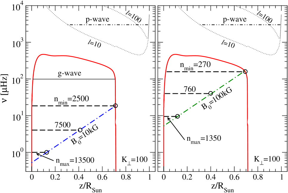
Figure 1: Relevant frequencies plotted against radial position within the sun. The solid curve gives the Brunt-Väisälä frequency, $N(z)$, while the dot-dashed lines are the Alfvén frequencies. Notice that $N(z)$ goes to zero at the solar center and the top of the radiative zone. The horizontal dashed lines represent the frequencies of magneto-gravity waves computed from Eq. (35) for several choices for the mode number, $n$, for fixed values $K_{x}=K_{\perp}=100$. As discussed in the text, resonances occur where the mode frequencies intersect the Alfvén frequency, indicated by circles in the figure. The two panels correspond to two choices for the magnetic field: 10 kG (left) and 100 kG (right). Minimum and maximum mode numbers are indicated, with $n_{\rm min}$ defined by the condition that its resonance occurs at the top of the radiative zone, $z_{r}(n_{\rm min})=0.7R_{\odot}$, and $n_{\rm max}$ having resonance at $z_{r}(n_{\rm max})=0.12R_{\odot}$ (see Figs. 4 and 5). The dotted lines denote acoustic (Lamb) frequencies for $l=10$ and $100$ (see [11]) while the double-dot-dashed horizontal line represents the trapping region for a p-wave of frequency 3000 $\mu$Hz and $l=10$. The horizontal solid line represents the trapping region for a g-wave of frequency 100 $\mu$Hz.

In the limit $B_{0}\to 0$ (and so $v_{A}\to 0$), Eq. (16) reduces to the standard evolution equation for ‘pure’ helioseismic $g$-modes, which is usually expressed in terms of the variable $v_{z}$ (which is related to $b_{z}$ through the relation $v_{z}=\omega b_{z}/k_{x}$). Since more detailed analyses – see Fig. 1 – show that $N$ rises from zero at the solar center, remains approximately constant $N\approx N_{0}$, through the radiative zone, and then falls to zero again at the bottom of the convective zone, these $g$-modes can be thought of as the eigen-modes of oscillations inside the cavity in between the two regions where $N$ goes through zero. For a given wave frequency, $\omega<N_{0}$, the turning points of this cavity are given by the condition $\omega\approx N$. For smaller $\omega$ the lower turning point gets closer to the solar center, $z\to 0$, and the upper one gets slightly closer to the bottom of the convective zone (CZ).

Conversely, if gravity is turned off ($N\to 0$), then Eq. (16) describes Alfvén waves, which oscillate with frequency $\omega=k_{x}v_{A}$ and propagate along the magnetic field lines. Notice that since $v_{A}\propto\rho^{-1/2}$ this frequency grows with $z$, since the density of the medium falls.

Keeping both magnetic and gravitational fields introduces qualitatively new behavior, as may be seen mathematically because equation (16) acquires a new singular point which occurs when the coefficient of the second-derivative term vanishes. Since this singularity appears at the Alfvén frequency,

$$\omega=k_{x}v_{A}$$ (18)

it can be interpreted as being due to a resonance between the $g$-modes and Alfvén waves. This resonance turns out to occur at a particular radius because the Alfvén frequency varies with radius while the $g$-mode frequency is independent of radius (see Fig. 1). The resonance occurs where the growing Alfvén mode frequency crosses the frequency of one of the $g$-modes, and the resulting waveforms would be expected to vary strongly at these points.

The resonance can occur inside the radiative zone if the Alfvén frequency climbs high enough to cross a $g$-mode frequency before reaching the top of the radiative zone. Since $v_{A}\propto B_{0}$, whether this occurs or not depends on the central field value, $B_{0}$. Our main task is to find the dependence of the spectrum of eigen-modes on magnetic field, and to elucidate when such singular resonances can appear within the Sun. Of particular interest for observational purposes is to know how the density and sound speed vary near the resonances, especially when the resonance region occurs near the locations of resonant neutrino oscillations.

The presence of a resonance at a particular radius, $z=z_{r}$, shifts the position of the upper turning points of the corresponding magneto-gravity wave towards deeper regions of the Sun. This leads to several new effects. First, the shortening of the cavity due to the presence of magnetic field causes the eigen-frequencies to depend on the magnetic field value. Second, there can be energy transfer between $g$-modes and Alfvén waves, within the narrow singular resonance layer, leading to the corresponding eigen-frequencies acquiring imaginary parts. Third, the nearer the upper boundary of MHD cavity is to the solar center, the stronger the $g$-modes are confined to the solar core.

More details of these waveforms can be obtained from a WKB-type analysis of the master Eq. (16). Near the solar center where $N^{2}\to 0$, if $(k_{x}v_{A})^{2}/\omega^{2}\ll 1$ one obtains the exponential solution $b_{z}\to e^{\pm k_{\perp}z}$. (Which combination of these solutions appears is fixed by boundary conditions, e.g. if $b_{z}(0)=0$ at the solar center we have $b_{z}\propto\sinh(k_{\perp}z)$.) One finds similar behaviour for the solution above the singular resonant layer, $z>z_{r}$, up to the top of the radiative zone. This exponential growth happens because of the exponential decrease of density (and so exponential increase in $v_{A}$) with $z$. The requirement for complex frequencies arises from the demand that the solution remain regular in the narrow Alfvén resonance layer.

3.2 Background Configurations

In order to acquire analytic solutions to eq. (16), we must specify a background profile for $\rho_{0}(z)$ and $g(z)$. We model $\rho_{0}(z)$ as an exponential density profile, $\rho_{0}(z)=\rho_{c}\,e^{-z/H}$ with $H$ constant, and take $g$ to be approximately constant. We now argue these to be reasonable approximations well inside the radiative zone, and not too close to the solar center.

The variation of background quantities may be characterized by the scale heights, $H_{A}^{-1}:=|(1/A_{0})(dA_{0}/dz)|$, for $A=\rho,p,T$ etc.. Solar models [2, 3, 30] show that the density scale height is the shortest in the radiative zone, $H_{g},~{}H_{T}>H_{\rho}$, and that $H_{\rho}$ takes the constant value $H_{\rho}=H=0.1\,R_{\odot}$ to a good approximation, except near the solar center and solar surface. On these grounds we have that the gravitational equation, $dg/dz=-4\pi G\,\rho_{0}$, implies $g=4\pi G\rho_{c}H\,\left(1-e^{-z/H}\right)$, which is approximately constant for $z$ much larger than $H$. For constant $g$ the hydrostatic equation, $dp_{0}/dz=-\rho_{0}\,g$, then implies $p_{0}=p_{c}\exp(-z/H)$ which also implies constancy of the temperature for gases obeying the ideal gas equation state, $p_{0}/\rho_{0}=RT_{0}/\mu$. Here $R$ is the gas constant, $R=k_{\scriptscriptstyle B}/m_{u}$, $\mu$ is the molecular weight measured in atomic mass units $m_{u}\simeq m_{p}$, and $k_{\scriptscriptstyle B}$ is Boltzmann’s constant. In terms of these quantities the density scale height becomes: $H=c^{2}/g$ (= constant) [2, 3], with $c=\sqrt{RT_{0}/\mu}$ being the isothermal sound velocity, which is related to the adiabatic sound velocity, $c_{s}$, by $c_{s}^{2}=\gamma c^{2}$. All of these quantities are constants within the approximations we are using.

Notice that our approximations that $\gamma$, $H=0.1R_{\odot}$ and $g$ are all constant also imply approximate constancy for the Brunt-Väisälä frequency, $N$, within the radiative zone.

3.3 Solution Using Hypergeometric Functions

Changing variables to $\xi=k_{x}^{2}v_{A}^{2}/\omega^{2}=\xi_{c}\,e^{z/H}$ we recast Eq. (16) as

$$(1-\xi)\xi^{2}\,\frac{d^{2}b_{z}(\xi)}{d\xi^{2}}+\xi\left(1-\xi-\frac{\gamma-1}{\gamma}\right)\frac{db_{z}(\xi)}{d\xi}+$$

$$+K_{\perp}^{2}(\kappa^{2}+\xi-1)\,b_{z}(\xi)=0~{},$$ (19)

where we introduce the dimensionless parameters $K_{\perp}^{2}=k_{\perp}^{2}H^{2}$, $\kappa^{2}=N^{2}/\omega^{2}$.

Since the equation (19) has three regular singular points – at $\xi=0,1$ and $\infty$ – it can be put into standard hypergeometric form,

$$\xi(1-\xi)\,\frac{d^{2}Y}{d\xi^{2}}+[c-(a+b+1)\xi]\,\frac{dY}{d\xi}-ab\,Y=0~{},$$ (20)

through a change of the dependent variable $b_{z}=\xi^{\sigma}\,Y(\xi)$. This permits an explicit solution for $b_{z}$ in terms of Gaussian hypergeometric functions, $F(a,b;c;\xi)={}_{2}F_{1}(a,b;c;\xi)$. Here the hypergeometric coefficients, $a,b$ and $c$, are given by

$$a=\sigma+K_{\perp},\qquad b=\sigma-K_{\perp},\qquad c=2\sigma+\gamma^{-1}~{},$$ (21)

where the complex index, $\sigma$, is defined by the expression

$$2\sigma=\frac{\gamma-1}{\gamma}-q~{},$$ (22)

with

$$q\equiv 1-c=\left[\left(\frac{\gamma-1}{\gamma}\right)^{2}-4K_{\perp}^{2}(\kappa^{2}-1)\right]^{1/2}~{}.$$

General Solutions

Two linearly-independent solutions to the Hypergeometric equation, (20), are

$$Y_{1}=F(a,b;c;\xi)~{},~{}~{}Y_{2}=\xi^{1-c}F(a-c+1,b-c+1;2-c;\xi)~{}.$$

These solutions must be analytic for all $\xi\neq 0,1$ and $\infty$, but they may acquire branch points at these three regular singular points depending on the values of $a$, $b$ and $c$. In the present case because $\mathop{\rm Re}\nolimits~{}(c-a-b)=\gamma^{-1}>0$, the solutions are bounded at $\xi=1$ as long as neither $c$ nor $2-c$ is zero or a negative integer. Moreover, the second fundamental solution, $Y_{2}$, is finite at $\xi=0$ if $\mathop{\rm Re}\nolimits~{}(1-c)=\mathop{\rm Re}\nolimits~{}q>0$.

We shall find that the waves of interest have complex frequencies, which we parameterize as $\omega=\omega_{1}(1+id)$ with $\omega_{1}$ and $d$ real, with $|d|\ll 1$. Complex $\omega$ implies, from (22), that the parameters $q$ (and so also $c$) are also complex, $q=q_{1}+iq_{2}$, with real and imaginary parts:

$$q=q_{1}+iq_{2}\equiv\sqrt{w_{1}+iw_{2}}=$$

$$\frac{1}{\sqrt{2}}\left[\sqrt{\sqrt{w_{1}^{2}+w_{2}^{2}}+w_{1}}+i~{}{\rm sgn}(d)\sqrt{\sqrt{w_{1}^{2}+w_{2}^{2}}-w_{1}}~{}\right]\,,$$ (23)

where $w_{1,2}$ are given by:

$$w_{1}=\left(\frac{\gamma-1}{\gamma}\right)^{2}+4K_{\perp}^{2}\left[1-\frac{N^{2}\,(1-d^{2})}{\omega_{1}^{2}\,(1+d^{2})^{2}}\right]~{},$$

$$w_{2}=\frac{8d\,N^{2}\,K_{\perp}^{2}}{\omega_{1}^{2}\,(1+d^{2})^{2}}~{}.$$

It is clear from these equations that one always has $\mathop{\rm Re}\nolimits~{}q=q_{1}>0$.

The general solution for $b_{z}(z)$ is therefore given by the linear combination of the independent solutions to Eq. (20):

$$b_{z}(z)=D_{1}\,\xi^{\sigma}F(a,b;c;\xi)+$$

$$+D_{2}\,\xi^{1-\sigma-1/\gamma}F(1+a-c,1+b-c;2-c;\xi)~{},$$ (24)

where one combination of the integration constants, $D_{1}/D_{2}$ is obtained by imposing boundary conditions at $\xi_{c}=\xi(z=0)$ and $\xi_{*}=\xi(z=z_{*})$, where $z_{*}\approx 0.7R_{\odot}$ denotes the top of the radiative zone.

Resonance Conditions

Although the solutions are bounded at the singular point $\xi=1$, they are generally not analytic there. The position $z_{r}$ determined by the condition

$$\hbox{Re}\,\xi(z_{r})=(k_{x}v_{A}(z_{r})/\omega_{1})^{2}=1$$ (25)

therefore defines the position of the $g$-mode/Alfvén resonance. This resonance occurs within the radiative zone only if $\xi_{c}<1$ and $\xi_{*}>1$. In this section we ask what this requires for the properties of the wave.

Expressed in terms of the central quantities, the Alfvén resonance condition is $\mathop{\rm Re}\nolimits~{}\xi(z_{r})=1$, or $\mathop{\rm Re}\nolimits~{}\xi_{c}=(k_{x}v_{Ac}/\omega_{1})^{2}=e^{-z_{r}/H}$. Since $0\leq z_{r}\leq z_{*}\approx 0.7R_{\odot}$ this condition limits the values of $K_{\perp}$ for which resonances can occur. Using the numerical values $H=7\times 10^{9}$ cm, $v_{Ac}=(B_{0}/43.4~{}\rm{G})$ cm s^-1 (obtained using the central density $\rho_{c}=150$ g cm^-3), $N=10^{-3}$ s^-1 (obtained using the mean acceleration $g=0.2$ km s^-2 and the ideal-gas adiabatic parameter $\gamma=5/3$), we find the following limits on the transverse wave number $K_{\perp}\geq K_{x}=k_{x}H$:

$$1\leq\frac{7\times 10^{6}\,(\omega_{1}/N)}{K_{x}(B_{0}/43.4~{}\rm{G})}\lesssim 30~{},$$ (26)

where the lower (upper) limit corresponds to the choice $z_{r}=0$ ($z_{r}=z_{*}\simeq 0.7R_{\odot}$).

For frequencies, $\omega_{1}\sim N$, and moderate central magnetic fields, $B_{0}\lesssim 100~{}G$, we see that the existence of a resonance requires the wave number $K_{\perp}$ to be large, $K_{\perp}\gg 1$. Smaller $K_{\perp}$ necessarily requires either larger magnetic fields or extremely low frequencies or both. Since we cannot, within the scope of our approximations, reduce the angular frequency lower than the solar angular rotation frequency (for which the Solar rotation period is $T_{\odot}\sim 27$ days), a reasonable lower limit for $\omega_{1}$ might be $\omega_{1}\sim 10^{-5}$ s^-1 (corresponding to a period $2\pi/\omega_{1}\sim 8$ days). Even for such small frequencies one finds from Eq. (26) the condition $3\times 10^{4}\gtrsim K_{\perp}\gtrsim 10^{3}$, as required.

Boundary Conditions

At the solar center ($z=0$ and so $\xi=\xi_{c}$) we use the boundary condition which would have arisen as a smoothness condition in cylindrical coordinates:

$$b_{z}(0)=k_{x}v_{z}(0)/\omega=0.$$ (27)

This requires the integration constants to satisfy

$$\frac{D_{2}}{D_{1}}=-\xi_{c}^{-q}\frac{F(a,b;c;\xi_{c})}{F(1+a-c,1+b-c;2-c;\xi_{c})}~{}.$$ (28)

This boundary condition is sometimes called the ‘total reflection’ condition because of the observation that it implies (for real $\omega$) that the reflection coefficient at $z=0$ equals unity: $R=|D_{2}/D_{1}|^{2}=1$. To see why this is so notice that real $\omega$ implies $q$ is pure real or pure imaginary. Within the domain of the approximation $k_{\perp}^{2}c_{s}^{2}/\omega^{2}\gg 1$ it is pure imaginary, so we write $q\to-i\beta$ for some real $\beta$. With this choice we have $\sigma\to(\gamma-1)/(2\gamma)+i\beta/2$, and so

$$a\to\sigma+K_{\perp},\qquad b\to\sigma-K_{\perp},\quad\hbox{and}\qquad c\to 1+i\beta~{},$$

which leads to the relations:

$$1+a-c \to \frac{\gamma-1}{2\gamma}+K_{\perp}-\frac{i\beta}{2}=a^{*}~{},$$

$$1+b-c \to \frac{\gamma-1}{2\gamma}-K_{\perp}-\frac{i\beta}{2}=b^{*}~{},$$

$$2-c \to 1-i\beta~{}=c^{*}.$$ (29)

From these conditions follows the conclusion $R=1$.

We next turn to the boundary condition at the top of the radiative zone, $z_{*}\approx 0.7R_{\odot}$. Since our interest is in resonant waves which lie deep in the radiative zone, we will assume $\xi_{*}=\xi(z_{*})\gg 1$ when applying this boundary condition.

The behaviour of $b_{z}$ for $\xi>1$ is found using Eq. (62) from Appendix A together with Eq. (24):

$$\frac{b_{z}}{D_{1}} = \left[A_{1}-(-)^{c}A_{3}\,\frac{D_{2}}{D_{1}}\right](-)^{-a}\xi^{-K_{\perp}}\times$$ (30)

$$\times F\left(a,1-c+a;1+a-b;\frac{1}{\xi}\right)+$$

$$+\left[A_{2}-(-)^{c}A_{4}\,\frac{D_{2}}{D_{1}}\right](-)^{-b}\xi^{+K_{\perp}}\times$$

$$\times F\left(1-c+b,b;1-a+b;\frac{1}{\xi}\right)~{},$$

where

$$A_{1}=\frac{\Gamma(c)\Gamma(b-a)}{\Gamma(b)\Gamma(c-a)},~{}~{}~{}~{}~{}A_{2}=\frac{\Gamma(c)\Gamma(a-b)}{\Gamma(a)\Gamma(c-b)},$$

$$A_{3}=\frac{\Gamma(2-c)\Gamma(b-a)}{\Gamma(b-c+1)\Gamma(1-a)},$$

$$A_{4}=\frac{\Gamma(2-c)\Gamma(a-b)}{\Gamma(a-c+1)\Gamma(1-b)}~{}.$$ (31)

For $\xi\gg 1$, the two terms in Eq. (30) behave as $\xi^{\pm K_{\perp}}\propto e^{\pm K_{\perp}\,z/H}$, and so either fall or grow exponentially as functions of $z$. We take the absence of the growing behaviour to be our boundary condition for $\xi=\xi_{*}$. This requires vanishing of the whole factor within brackets in the second line of Eq. (30), thereby providing a second condition which must be satisfied by the ratio $D_{2}/D_{1}$:

$$\frac{D_{2}}{D_{1}}=(-)^{-c}\;\frac{\Gamma(c)\Gamma(1-b)\Gamma(1+a-c)}{\Gamma(2-c)\Gamma(a)\Gamma(c-b)}~{}.$$ (32)

Given this boundary condition, $b_{z}$ falls exponentially for $z>z_{r}$, $b_{z}\sim\xi^{-K_{\perp}}=\xi_{0}^{-K_{\perp}}e^{-K_{\perp}z/H}$, as given by the first line in Eq.(30).

3.4 Eigenfrequencies

The consistency of the two conditions, eqs. (32) and (28), for $D_{2}/D_{1}$ gives the eigenvalue condition which fixes the dispersion relation for the resonant waves:

$$\xi_{c}^{-q}\frac{F(a,b;c;\xi_{c})}{F(1+a-c,1+b-c;2-c;\xi_{c})}=$$

$$=-(-)^{-c}\;\frac{\Gamma(c)\Gamma(1-b)\Gamma(1+a-c)}{\Gamma(2-c)\Gamma(a)\Gamma(c-b)}~{},$$ (33)

from which we read off the MHD frequency, $\omega(k_{x},k_{y},B_{0},n)$, where the integer $n$ is the mode number for the eigenfunction of interest. The solutions which are obtained in this way have the important property that they are complex, $\omega=\omega_{1}\,(1+id)$, a feature which is also present in the absence of gravitational loading, and which has been exploited in other contexts in attempts to explain the nature of coronal heating [18, 19, 20, 16, 17].

We note in passing that, in contrast to the master equation in (16), Eq. (3.4) does not reduce to the standard $g$-mode spectrum in the limit $B_{0}\to 0$. It does not do so because of our assumption that $N$ be approximately constant. Although this approximation suffices for the study of MG waves, it is too crude to capture the resonant frequencies of $g$-modes. It cannot do so because $g$-modes are trapped inside the radiative zone precisely because $N$ is not constant, but instead drops to zero at the top of the radiative zone. For MG waves this dropping of $N$ is not crucial because its role in trapping the modes is instead played by the resonant layer at $z=z_{r}$.

The eigenvalue condition can be written in a more transparent way by taking advantage of some properties of hypergeometric functions. Recall that our interest is in the regime $K_{\perp}N/\omega_{1}\gg 1$, and so the parameter $q$, as defined by Eq. (22), is mostly imaginary, $q=-i\beta$, since $|d|\ll 1$, with $\beta=2K_{\perp}N/\omega\gg 1$. This implies that $\sigma=(\gamma-1)/(2\gamma)+i\beta/2$ is also large inasmuch as $|\sigma|\gg 1$, and so must also be $a$ and $b$. This observation allows us to use the Watson asymptotic form for hypergeometric functions (Appendix A. Some Hypergeometric Facts) – see Appendix A – which applies for large values of $a$ and $b$.

Using this, together with liberal use of the convolution identity $\Gamma(z)\Gamma(1-z)=\pi/\sin(\pi z)$, allows us to rewrite the eigenvalue condition, Eq. (3.4), as a simple transcendental equation:

$$-2i\beta\ln\eta=2i\pi n+\ln\left|\tan\frac{\pi}{\gamma}\right|\pm i\pi\left(\frac{1-\gamma}{\gamma}\right)~{},$$ (34)

where the upper (or lower) sign on the right-hand-side is chosen if the imaginary part of the frequency is positive: $d>0$ (or negative, $d<0$). The variable $\eta$ is defined by $\eta=\xi_{c}^{-1/2}-\sqrt{1/\xi_{c}-1}$, and depends on the magnetic field ${\bf B}_{0}$ through the Alfvén velocity $v_{Ac}$, since $\xi_{c}=(k_{x}v_{Ac}/\omega_{1})^{2}$. The integer $n=0,\pm 1,\pm 2,...$ is the mode number.

The eigenvalue equation is easier to work with if re-expressed slightly. Solving for $\xi_{c}(\eta)$ we find $\xi_{c}^{1/2}=2\eta/(1+\eta^{2})=k_{x}\,v_{Ac}/\omega$, and so

$$\beta=-\left(\frac{4HN}{\alpha\,v_{Ac}}\right)\;\frac{\eta}{1+\eta^{2}}$$

where $\alpha=k_{x}/k_{\perp}\leq 1$. If we now change variables to $\chi$ defined by $\eta=e^{-\chi}$ we find

$$\chi=\frac{\alpha\,v_{Ac}}{4NH}\left[2\pi n-i\ln\left|\tan\frac{\pi}{\gamma}\right|\pm\pi\left(\frac{1-\gamma}{\gamma}\right)\right]\cosh\chi~{}.$$ (35)

The variable $\chi$ is convenient because physical quantities have simple expressions in terms of it. In particular, the phase velocity is $v_{ph}=\omega_{1}/k_{x}=v_{Ac}\mathop{\rm Re}\nolimits\cosh\chi$; the frequency’s imaginary part is determined by $d=\mathop{\rm Im}\nolimits\cosh\chi/\mathop{\rm Re}\nolimits\cosh\chi$, and the position of the resonant layer is $z_{r}=2H\ln\left[\mathop{\rm Re}\nolimits\cosh\chi\right]$.

Notice that Eq. (35) takes the form $\chi=A\cosh\chi$. For real $A$ this equation has two real roots for $\chi$ if $A<A_{max}$ and none if $A>A_{max}$, where $A_{max}$ is defined as the maximum value taken by the function $\chi/\cosh\chi$ (which numerically occurs for $\chi=\chi_{max}=1.1997)$. A similar result holds for $A$ and $\chi$ close to real, such as happens when $\omega=\omega_{1}(1+id)$, and so solutions with $d$ small only exist up to a maximum mode number, $|n|\leq n_{max}$, where

$$n_{max}=\left(\frac{2NH}{\pi\alpha\,v_{Ac}}\right)\frac{\chi_{max}}{\cosh\chi_{max}}~{}.$$

Solutions with large $d$ must be discarded because they lie beyond the scope of the linearized approximations within which we work.

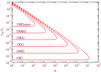
Figure 2: Plot of the $v_{ph}/c_{s}=\omega_{1}/k_{x}c_{s}$ against mode number, $n$, where $c_{s}$ is the adiabatic sound speed and $\omega_{1}$ is the real part of the eigenfrequencies, $\omega=\omega_{1}(1+id)$, as predicted by Eq. (35). Different curves correspond to different background magnetic field strengths, ${B}_{0}$. Solid lines represent resonances which are inside the radiative zone, whilst dashed lines correspond to unphysical modes whose resonances lie outside of the radiative zone.

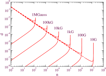
Figure 3: Plot of the $d$ against mode number, $n$, where $d$ gives the imaginary part of the eigenfrequencies, $\omega=\omega_{1}(1+id)$, as predicted by Eq. (35). Different curves correspond to different background magnetic field strengths, ${B}_{0}$. Solid lines represent resonances which are inside the radiative zone, whilst dashed lines correspond to unphysical modes whose resonances lie outside of the radiative zone.

Figures 2 and 3 present our numerical solution of the eigenvalue spectrum obtained from Eq. (35). Figure 2 plots $v_{ph}(n)/c_{s}=\omega_{1}/(c_{s}k_{x})$ vs mode number $n$ for various magnetic fields, $B_{0}$. Figure 3 similarly plots $d$ against mode number for the same magnetic fields. In both plots the parameter $\alpha=K_{x}/K_{\perp}$ is taken to be unity, $\alpha=1$. The result with $\alpha\neq 1$ is trivially found by rescaling $B_{0}$ because Eq. (35) depends only on the product $\alpha B_{0}$. In both figures a dashed line is used if the resonance of interest occurs above the top of the radiative zone (and so outside the domain of many of our approximations).

Both of the figures 2 and 3 show two branches of solutions up to a maximum mode number, as expected. Their dependence on $n$ can also be understood analytically if we take $\mid\chi\mid\gg\xi_{c}\sim 1$, and so $\eta\ll 1$. In this limit we obtain from (34) the following approximate equation for the MHD spectrum:

$$\frac{\omega_{1}}{N}=\frac{2K_{\perp}}{\pi n}\,\left(z_{r}/2H+\ln 2\right)~{},$$ (36)

$$d=\frac{\ln|\tan(\pi/\gamma)|}{2\pi n\left(1-(z_{r}/2H+\ln 2)^{-1}\right)}~{},$$

which leads to the asymptotic solution

$$\frac{\omega_{1}}{N}=\frac{2K_{\perp}}{\pi n}\ln\left(\frac{4NH}{\alpha v_{Ac}}\frac{1}{\pi n}\right),$$

$$d=\frac{\ln\left|\tan(\pi/\gamma)\right|}{2\pi n}~{}.$$ (37)

These modes correspond to the branches of the figures 2 and 3 for which both $v_{ph}/c_{s}$ and $d$ fall with $n$. The other branch can be found by using the approximation $|\chi|\ll 1$ and hence $\cosh\chi\approx\allowbreak 1+\chi^{2}/2$. The spectrum in this case is

$$\omega_{1}=\frac{\alpha K_{\bot}v_{Ac}}{H},$$

$$d=-\left(\frac{\alpha v_{Ac}}{4NH}\right)^{2}\pi n\ln\left|\tan\frac{\pi}{\gamma}\right|~{}.$$ (38)

Note that for this branch $v_{ph}(n)/c_{s}$ is independent of the mode number, $n$, and $d$ grows with $n$, as is also seen in the figure.

In addition to requiring the resonance to occur in the radiative zone (the solid line in the figures), the validity of our approximations also demand the frequency to not be smaller than $10^{-5}$ s^-1 due to our neglect of the 27-day period solar rotation. Inspection of Fig. 2 shows that these two conditions are consistent with one another for a reasonably large range of modes only for magnetic fields larger than a kG or so.

4 The Resonant Properties

Several striking features emerge from the previous section’s analysis of the hydrodynamic eigenvalues and eigenfunctions. The main two of these are:

1. The eigenfrequencies predicted by Eq. (34) are complex, implying both damped and exponentially-growing modes, and

2. The eigenmodes are not smooth as functions of $z$ about the singular resonant point, $z=z_{r}(n,k_{x},k_{y})$, whose position depends on the quantum numbers of the mode in question.

These features lie at the root of the surprisingly large effects which are produced by even moderate magnetic fields. We have argued that both of these features can be traced to a resonance between $g$-modes and Alfvén waves, which arises due to the existence of gradients in the background density, $\rho_{0}(z)$.

In this section we expand on these two properties, to more precisely pin down their origin. In particular, we expect the development of complex frequencies to indicate a hydrodynamical instability. This is much like the imaginary part which $g$-waves develop as one passes into the convective zone from the radiative zone. For $g$-modes this imaginary part arises because buoyancy no longer acts as a restoring force in the convective zone, but instead becomes destabilizing. Indeed the instability in this case drives the convection, which is why the radiative zone ends. We expect a similar instability to arise for the Alfvén/$g$-mode resonance.

4.1 Instability

The necessity for complex frequencies is the most disturbing feature about the above eigenvalue problem, because it implies mode functions which grow exponentially in amplitude with time. This signals an instability in the physics which pumps energy into these resonances, and this section aims to discuss the nature of this instability, and the physical interpretation to be assigned to the imaginary part, $d$.

Exponentially-growing instabilities within an approximate (e.g. linearized) analysis reflect a system’s propensity to leave the small-field regime, on which the validity of the approximate analysis relies. The question becomes: where does the instability lead, and what previously-neglected effects stabilize the runaway behaviour?

In the present instance we shall see that the normal modes become strongly peaked near the resonant radii, and that the energy flow near these radii is directed along the resonance plane, as would be true for a pure Alfvén wave. This leads us to the following picture. Since helioseismic waves are likely generated by the turbulence at the bottom of the convective zone, it is natural to imagine starting the system with a regular helioseismic $g$-mode and asking how it evolves. In this case the resonance allows the energy in this mode to be funnelled into the Alfvén wave, and so to be channelled along the magnetic field lines away from the solar equatorial plane. This process drives us beyond the range of our approximations by making the wave amplitude large near the resonant surface, but also by driving energy out of the equatorial plane where the rectangular analysis applies.

We arrive in this way at an interpretation in which the instability signals the excitation of Alfvén waves from $g$-modes due to their resonant mixing. In this picture the imaginary part of the frequency, $\Gamma=\mathop{\rm Im}\nolimits\,\omega=d\,\omega_{1}$, describes the rate at which the Alfvén mode is excited in this process. Since the mixing and excitation are weak-field hydrodynamic phenomena it is reasonable that this rate can be computed using only the linearized magneto-hydrodynamical equations.

Once excited, the mode amplitudes near the resonances grow until the energy in them becomes dissipated by effects which are not captured by the approximate discussion we present here. The rate for this dissipation must grow as the mode amplitude grows, until it equals the production rate, $\Gamma$, at which point a steady state develops and the mode growth is stabilized. Because the resonant mode grows until its damping rate equals its production rate, it suffices to know the mode’s growth rate in order to determine the overall on-resonance amplitude.

How much more can be said about the amplitude of the modes depends on whether or not the mode stabilizes at small enough amplitudes to allow the hydrodynamic approximation to the production rate, $\Gamma=d\,\omega_{1}$, to be accurate. For instance, if the mode only stabilizes once it is large enough to require a nonlinear analysis, then the final production and dissipation rates may be very different from the linearized expressions derived above. If, on the other hand, the modes saturate at comparatively small amplitudes by dissipating energy into non-hydrodynamical modes (such as by Landau damping), then it can happen that the stabilized mode amplitude is not large enough to significantly change the linearized prediction for its production rate.

In what follows we use the imaginary part of $\omega$ to determine the resonant mode’s amplitude at the position of the resonance. There is no loss in doing so to the extent that we take $\mathop{\rm Im}\nolimits\omega$ as a parameter which is not related to the mode quantum numbers by the hydrodynamical equations of motion. On occasion we shall also use the explicit formulae for $\mathop{\rm Im}\nolimits\omega$ which is predicted by the hydrodynamics, and in this case we are assuming that the mode stabilization occurs at small enough amplitudes to not invalidate the assumption that this is a good approximation to the mode production rate.

4.2 Spatial dependence

We next address the singular shape of the wave fronts at the resonant points, $z=z_{r}$. Mathematically, this singularity arises because the interval of physical interest, $0\leq z\leq z_{*}$, corresponds to the interval $0<\xi_{c}\leq\xi\leq\xi_{*}$, and this contains the singular point $\xi=1$ provided $\xi_{c}<1$ and $\xi_{*}>1$. The hypergeometric functions can – and do – develop singularities at $\xi=1$, and it is this singular behaviour which we now examine.

Using Eq. (Appendix B. Asymptotic Forms) of the Appendix B one finds as $\xi\to 1$ (from either side):

$$b_{z}\propto|\xi-1|^{1-\nu}+\hbox{nonsingular}\quad\hbox{and}\quad\frac{db_{z}}{dz}\propto|\xi-1|^{-\nu},$$ (39)

with $\nu=(\gamma-1)/\gamma$ (giving $\nu=\frac{2}{5}$ for an ideal gas, for which $\gamma=\frac{5}{3}$). For $0<\nu<1$ we see that $b_{z}$ remains finite but $db_{z}/dz\to\infty$ as $\xi\to 1$. As we shall see, once the eigenfrequency’s imaginary part is included $db_{z}/dz$ does not actually diverge as $\xi\to 1$, but instead adopts a systematically large resonant line-shape.

Using this information in eqs. (14) allows the asymptotic form for all other quantities to be determined at the resonant point. In particular, since $v_{z}$ does not involve $db_{z}/dz$, it also remains finite on resonance, unlike all other components of the fluid velocity. This indicates that it is the transverse velocity perturbations (and so also the transverse kinetic energy of the oscillations) which increase most dramatically at the resonant plane.

Positions of resonances

The equation for the position of resonances can be found by using the resonance condition

$$\hbox{Re}~{}\xi=\hbox{Re}~{}\xi_{c}\;e^{z/H}=\left(\frac{k_{x}v_{Ac}}{\omega_{1}(n)}\right)^{2}e^{z_{r}(n)/H}=1$$ (40)

and Eq. (36). It takes the following transcendental form

$$z_{s}(n)=H\left[\frac{K_{x}}{K_{\perp}}\left(\frac{\pi|n|\,v_{Ac}}{c_{s}}\right)\frac{\gamma}{\sqrt{\gamma-1}}\;e^{z_{s}(n)/2H}-\ln 4\right]\,.$$ (41)

Taking into account the asymptotic form for the real part of the eigenfrequency, $\omega_{1}(n)$, as given by Eq. (3.4), leads to the following asymptotic expression for the dependence of the resonant layer position on the node number, $n$:

$$z_{r}(n)=2H\ln\left[\frac{4NH}{\alpha v_{Ac}}\frac{1}{2\pi n}\ln\left(\frac{4NH}{\alpha v_{Ac}}\frac{1}{\pi n}\right)\right]\,,$$ (42)

here

$$v_{Ac}=\frac{B_{0}}{\sqrt{4\pi\rho_{c}}}=\left(\frac{B_{0}}{43.4~{}\hbox{G}}\right)\;\hbox{cm s}^{-1}$$ (43)

is the Alfvén velocity at the solar center.

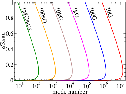
Figure 4: A plot of the resonant position, $z_{r}(n)$, vs mode number $n$ for different magnetic fields in the range $B_{0}=$ 10G–1MGauss.

Fig. 4 plots the position, $z_{r}(n)$, predicted by Eq. (42) for the case of longitudinal wave propagation ($k_{y}=0$) and for magnetic fields in the range $B_{0}=$10G–1MGauss. (The same result for an obliquely-propagating wave with $k_{y}\neq 0$ is produced by a larger value for $B_{0}$.) This plot is the analog of Figs. 5a,b in [14].

Spacing of resonances

Knowing the position of the resonances also permits us to determine the distance between them. This quantity is relevant to the propagation of particles like neutrinos through the resonant waves. The spacing is:

$$z_{r}(n+1)-z_{r}(n)=\left(\frac{K_{x}}{K_{\perp}}\right)\frac{\pi H\,v_{Ac}\gamma}{c_{s}\sqrt{\gamma-1}}\;e^{z_{r}(n)/2H}~{}.$$ (44)

This dependence of this quantity on mode number, $n$, is shown in Fig. 5 for longitudinal wave propagation, $k_{y}=0$, and for different magnetic field values. From this figure we see, in the region $z_{r}\gtrsim 0.3R_{\odot}$, that the distance between layer positions grows with magnetic field and with distance from the solar center. Both of these features were already seen in preliminary WKB calculations of the resonances (see Figs. 7a, 7b of ref. [14]), and our present numerics also confirm that the spacing is approximately proportional to $B_{0}$ for $z\gtrsim 0.3R_{\odot}$, that was seen earlier.

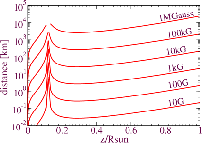
Figure 5: The distance between neighbouring Alfvén resonant layers vs the position of the layer within the solar interior.

Eq. (44) can be simplified using the expression, Eq. (42), for the resonance position:

$$z_{r}(n+1)-z_{r}(n)\approx\frac{2H}{\mid n\mid}~{},$$ (45)

where the inverse mode number $\mid n\mid^{-1}$ is proportional to the background magnetic field $\sim B_{0}$. This is in accordance with the spectrum Eq. (36), for which the phase velocity $v_{ph}=\omega_{1}/k_{x}$ equals the Alfvén speed at the resonance position, $\omega_{1}/k_{x}=v_{A}(z_{r},B_{0})\sim B_{0}$.

Numerically, it is noteworthy that the spacing between resonances can be in the ballpark of hundreds of kilometers. This is significant because this is close to the resonant oscillation length, $l_{osc}^{res}$, for $E\sim\rm{MeV}$ neutrinos, if – as now seems quite likely – resonant LMA oscillations are responsible for explaining the solar neutrino problem since

$$l_{osc}^{res}=\frac{250~{}\rm{km}~{}(E/\rm{MeV})}{\Delta m^{2}_{5}\sin 2\theta}\,,$$ (46)

where $\Delta m^{2}_{5}=\Delta m^{2}/10^{-5}~{}\hbox{eV}^{2}$. Repeatedly perturbing neutrinos over distance scales comparable to $l_{osc}^{res}$ has long been known to be a prerequisite for disturbing the standard MSW picture of oscillations in the solar medium. This raises the possibility – recently explored in more detail in ref. [8] – that $g$-mode/Alfvén resonances can alter neutrino propagation. If so, the observation of resonant oscillations of solar neutrinos may provide some direct information about the properties of the MG waves we discuss here.

Widths of the resonance layers

We next examine the energy flow in the vicinity of a resonance. This gives some information about the nature of the instability which is indicated by the complex mode frequencies. We find here that there is a large energy flow along the magnetic field lines, perpendicular to the $z$ direction. We use the dimension of the region in which this energy flows as a measure of the width of the resonant layer.

In the linearized regime the energy flux, ${\bf{S}}$, has both mechanical and electromagnetic (Poynting) components, ${\bf{S}}={\bf{S}}_{\rm mech}+{\bf{S}}_{\rm em}$, with

$${\bf{S}}_{\rm mech} = p^{\prime}\,{\bf{v}}~{},$$ (47)

$${\bf{S}}_{\rm em} = \frac{1}{4\pi}\,\left\{\Bigl{[}{\bf{B}}^{\prime}\times[{\bf{v}}\times{\bf{B}}_{0}]\Bigr{]}\right\}.$$

In order of magnitude, the relative size of these contributions is $B_{0}B^{\prime}/(4\pi p^{\prime})$ and this turns out to be small. This smallness is easy to see to the extent that $B^{\prime}/B_{0}\sim p^{\prime}/p_{0}$, since then $B_{0}B^{\prime}/(4\pi p^{\prime})\sim B_{0}^{2}/(4\pi p_{0})$, which is small by virtue of the background inequality $B^{2}_{0}/(4\pi)=\gamma\,(v_{A}^{2}/c_{s}^{2})\,p_{0}\ll p_{0}$.

Since the mechanical energy flux dominates, its direction is simply given by the direction of ${\bf{v}}$ near the resonance. This may be determined using the asymptotic form as $\xi\to 1$ in the expressions for $p^{\prime}$ and $v_{z}$ in eqs. (14). Notice that $v_{z}$ approaches a finite value in this limit, while $v_{x},v_{y}$ and $p^{\prime}$ all diverge as $\xi\to 1$. This shows that the energy flow, like the fluid flow, is mainly parallel to the resonant plane when evaluated near a resonance.

Using the asymptotic expressions, $db_{z}(z)/dz\sim{\cal B}\;|1-\xi|^{-\nu}$, and $b_{z}(z)\sim{\cal B}\;|1-\xi|^{1-\nu}+{\cal C}$, with constants ${\cal B}$, ${\cal C}$ and $\nu=(\gamma-1)/\gamma\approx 0.4$, we obtain $v_{z}\propto|b_{z}|\sim{\cal B}\,|1-\xi|^{1-\nu}$, and

$$p^{\prime},v_{x},v_{y}\propto\left|\frac{db_{z}}{dz}\right|\sim\frac{|{\cal B}|}{|1-\xi|^{\nu}}=$$ (48)

$$=\frac{|{\cal B}|}{|1-\xi_{r}+\xi_{r}2id|^{\nu}}~{}=\frac{|{\cal B}|}{[(1-\xi_{r})^{2}+4\,\xi_{r}^{2}d^{2}|^{\nu/2}}~{},$$

where we have used our definitions – $\omega=\omega_{1}(1+id)$, with $|d|\ll 1$, and so $\xi=\xi_{r}(1-2id)$, with $\xi_{r}=\Bigl{(}{k_{x}v_{Ac}/\omega_{1}}\Bigr{)}^{2}e^{z_{r}/H}$ – to write the real and imaginary parts explicitly. The energy flow near the resonant plane is similarly given by the time average ${\bf{S}}=\langle p^{\prime}{\bf{v}}\rangle=\frac{1}{2}{\rm Re}(p^{\prime}{\bf{v}}^{*})$, where the symbol $\langle\cdots\rangle$ means average over time. Combining the results for $p^{\prime}$ and ${\bf{v}}$ we see that near resonance

$$S_{z} \propto \frac{1}{[(1-\xi_{r})^{2}+4\,\xi_{r}^{2}d^{2}]^{\nu/2}}~{},$$

$$S_{x},S_{y} \propto \frac{1}{[(1-\xi_{r})^{2}+4\,\xi_{r}^{2}d^{2}]^{\nu}}~{}$$ (49)

and so, for instance, $S_{z}$ reaches half of its resonant value when $\xi=\xi_{\pm}=1\pm\delta\xi$ where $[(1-\xi_{\pm})^{2}+4\,\xi_{\pm}^{2}d^{2}]^{\nu/2}=2(2d)^{\nu}$.

On the other hand, for $z$ well beyond the resonant zone, where $\xi>1$, we know that $b_{z}(z)$ is given by Eq. (30), which states $b_{z}(z)\propto\xi^{-K_{\perp}}F(a,a^{*};1+2K_{\perp};\xi^{-1})$. By virtue of the condition $a^{*}=1-c+a$ we see that this is a real function (in the limit $d\to 0$). Consequently, the explicit factors of ‘$i$’ in eqs. (14) imply that quantities like the pressure perturbation, $p^{\prime}(z)$, and the transverse velocities $v_{x,y}(z)$ are pure imaginary. It therefore follows that the $z$-component of the energy flux vanishes in the region $z>z_{r}$, outside of the resonance, because $S_{z}=\frac{1}{2}{\rm Re}(p^{\prime}v_{z}^{*})=0$, while the transverse components are nonzero in this region, but are falling off exponentially.

This peaking, then vanishing, of $S_{z}$ motivates our choice of the width of the $S_{z}(z)$ resonant line-shape as a measure of the resonance layer width. From this condition we can easy find the results for the widths $z_{\pm}$ (or, equivalently, $\xi_{\pm}$):

$$\delta\xi^{2}=(2|d|)^{2}\,\left(2^{2/\nu}-1\right)~{},$$ (50)

giving our final expression for the width of the Alfvén singular layer:

$$\delta z=z_{+}-z_{-}=H\ln\left({\frac{\xi_{+}}{\xi_{-}}}\right)\approx 4H|d|2^{\gamma/(\gamma-1)}~{}.$$ (51)

Substituting the expression for $d$ in terms of mode number, using Eq. (3.4), this becomes

$$\Delta z_{r}(n)\approx\frac{2H}{\pi n}2^{\gamma/(\gamma-1)}\ln\left|\tan\frac{\pi}{\gamma}\right|~{}.$$ (52)

Figure 6: A plot of neighboring density profiles, showing their width in comparison with the spacing in between them. The plot is done for resonances in the region $z_{r}\sim 0.3R_{\odot}$.

Together with Eq. (45) we then get the ratio of the distance between resonances to the width of each resonance,

$$\frac{z_{r}(n+1)-z_{r}(n)}{\Delta z_{r}(n)}=\frac{\pi}{2^{\gamma/(\gamma-1)}\ln\mid\tan\frac{\pi}{\gamma}\mid}\approx 0.5~{}.$$ (53)

Figure 6 plots the density profiles of two neighboring resonances in the region $z_{r}\sim 0.3R_{\odot}$. In this region their width is approximately twice their separation as measured by the distance between peaks. That is not surprising since the shape of the density profile is the same as in Eq. (48) for other MHD perturbations (see below, Eq. (55)).

Density Profiles

We now give the explicit expression for the density profile predicted for our wave solutions. The basic expression is obtained through the direct substitution of our expression for $b_{z}(z)$ – keeping in mind eqs. (24), (28) and (3.3) – into the last of eqs. (14). We find in this way the following expression for $\rho^{\prime}/\rho_{0}$, divided by the arbitrary wave normalization, $D_{1}$:

$$\frac{1}{D_{1}}\left(\frac{\rho^{\prime}(z)}{\rho_{0}(z)}\right)=$$

$$=\frac{-i\xi_{c}^{\sigma_{1}}}{k_{x}H}\left\{\left(\frac{\gamma-1}{\gamma}+\frac{\sigma_{1}\omega^{2}}{k_{\perp}^{2}c_{s}^{2}}\right)\left(\frac{\xi}{\xi_{c}}\right)^{\sigma_{1}}F(a_{1},b_{1};c_{1};\xi)\right.$$

$$-\left(\frac{\gamma-1}{\gamma}+\frac{\sigma_{2}\omega^{2}}{k_{\perp}^{2}c_{s}^{2}}\right)\Bigl{(}\frac{\xi}{\xi_{c}}\Bigr{)}^{\sigma_{2}}F(a_{2},b_{2};c_{2};\xi)\frac{F(a_{1},b_{1};c_{1};\xi_{c})}{F(a_{2},b_{2};c_{2};\xi_{c})}$$

$$+\frac{\xi_{c}\omega^{2}}{k_{\perp}^{2}c_{s}^{2}}\left[\frac{(\sigma_{1}^{2}-K_{\perp}^{2})}{1+i\beta}\left(\frac{\xi}{\xi_{c}}\right)^{\sigma_{1}+1}F(a_{1}+1,b_{1}+1;c_{1}+1;\xi)\right.$$

$$-\frac{(\sigma_{2}^{2}-K_{\perp}^{2})}{1-i\beta}\;\left(\frac{\xi}{\xi_{c}}\right)^{\sigma_{2}+1}F(a_{2}+1,b_{2}+1;c_{2}+1;\xi)\times$$

$$\left.\left.\times\frac{F(a_{1},b_{1};c_{1};\xi_{c})}{F(a_{2},b_{2};c_{2};\xi_{c})}\right]\right\}\,,$$ (54)

where $\sigma_{1}$ is given by Eq. (22) for $q=-i\beta$, $\sigma_{2}=(\gamma-1)/2\gamma-i\beta/2$; $a_{1,2}=\sigma_{1,2}+K_{\perp}$, $b_{1,2}=\sigma_{1,2}-K_{\perp}$; $c_{1,2}=1\pm i\beta$ (see Eq. (3.3)).

The behaviour of the density perturbation near the resonant point, $z_{r}$, takes a simpler form for the Lagrange perturbation

$$\delta\rho(\vec{r})=\rho^{\prime}(\vec{r})+\delta\vec{r}\cdot\nabla\rho_{0}=$$

$$=[\rho^{\prime}(z)-(\delta z/H)\rho_{0}(z)]e^{-i(\omega t-k_{x}x-k_{y}y)},$$ (55)

where the Eulerian perturbation $\rho^{\prime}(z)$ is given by Eq. (4.2). In linear MHD the Lagrangian density perturbation is directly constrained by mass conservation, Eq. (1), $-i\omega\rho_{0}^{-1}\delta\rho(z)=-u$, where $u={\rm div}\,{\bf{v}}$ is the compressibility, given by Eq. (15). One obtains in this way the following Lagrange density perturbation near the resonance, $z\sim z_{r}(n)$:

$$\frac{1}{D_{1}}\frac{\delta\rho(z)}{\rho_{0}}\approx C-\left[e^{-(z-z_{r}(n))/H}(1+2id)-1\right]^{-{(\gamma-1)}/{\gamma}}\,,$$ (56)

where

$$C=\frac{\Gamma(\gamma^{-1})}{\Gamma(-\gamma^{-1})}\left(\frac{\gamma v_{ph}(n)}{i\sqrt{\gamma-1}\;c_{s}}\right)^{2/\gamma}\left(\frac{\gamma-1}{4\gamma}+\frac{\gamma^{2}K_{\perp}^{2}}{\gamma-1}\right)\,.$$

Here the phase velocity, $v_{ph}(n)=\omega_{1}(n)/k_{x}$, is given by the solution to the eigen-spectrum, $\omega=\omega_{1}(1+id)$, such as obtained in Eq. ((3.4)), and we include the unknown normalization factor $D_{1}$.

This quantity $\left|\delta\rho/\rho_{0}\right|$ is plotted in Fig. 6 for two neighbouring resonances near $z=0.3R_{\odot}$ for the two values of the magnetic field, $B_{0}=$10kG and $B_{0}=$100kG. We see that the presence of the resonances introduces a series of density excursions, located at the resonant positions. The disappearance of the resonant density spikes in the zero-field limit is most easily seen by noticing that in the limit $B_{0}\to 0$ the position $z_{r}$ becomes negative, $z_{r}=-H\ln 4<0$ (see Eq. (41)), or occurs outside the physical region $0\leq z\leq z_{*}$.

5 Possibilities for Observations

Given the strength of the resonant effects on the helioseismic wave profiles, we next explore some of their observable properties to determine how they might be detected, and to what extent their effects are consistent with current helioseismic observations.

5.1 Measurements of Mode Frequencies?

Many helioseismic waves have been detected, but to date all of these are pressure-driven $p$-modes rather than the usually-lower-frequency $g$-modes. The latter are more difficult to detect because they are so strongly attenuated within the convective zone.

Because the central Alfvén frequency is so small compared with the other helioseismic frequencies, we only expect resonances between Alfvén waves and those helioseismic waves which penetrate most deeply into the solar interior, and which have the lowest frequencies. This is why the resonance we have found involves mixing only with $g$-modes, and not $p$-modes. It follows that so long as observations are restricted to $p$-modes, the resonances we describe here will have negligible implications for the comparison between measured $p$-wave frequencies and solar models.

Things become more interesting should $g$-modes be observed, since then a comparison between observations and predicted frequencies could depend more strongly on the solar magnetic field. Figure (2) (or Eqs. (3.4) and (42)) show how the frequencies of the resonant modes depend on magnetic field. Unfortunately, frequencies this low are likely to be a challenge to detect for quite some time.

Of course, a proper comparison requires the inclusion of the full (spherical) geometry of the problem, as well as temperature and gravity gradients, solar rotation, and other factors which we ignore here. Our goal in this paper is merely to point out the potential for larger-than-expected effects, and to obtain a rough first determination of the sensitivity to magnetic fields.

5.2 Constraints on Mode Amplitudes

Mode amplitude remains undetermined within the linear approximations assumed here, and is ultimately controlled by the mechanisms which stimulate and damp the waves of interest in the solar environment. Amplitude can nevertheless be characterized in any of three equivalent ways: the size of the mode’s contribution to the mass-density profile, the size of the fluid velocity, $v_{z}$, at the solar surface, and the total mode energy. In principle, our solutions can be used to express any two of these in terms of the third, as functions of the background magnetic field.

A sufficiently detailed comparison of the resulting expressions – should this become possible – would then allow one to obtain the magnetic field strength. We illustrate this by calculating here the energy content of the resonant MG waves.

Mode Energy

The mode energy is a useful way to quantify the mode amplitude. Here we provide formulae which make this connection explicit. The mode energy is most simply computed by using the virial theorem, which relates the total energy to the kinetic energy averaged over a single period of oscillations: $E=2\langle E_{\rm kin}\rangle$:

$$\langle E_{\rm kin}\rangle=\frac{1}{2}\int d^{3}{\bf{x}}\;\rho_{0}\,\langle[\hbox{Re}~{}{\bf{v}}({\bf{x}},t)]^{2}\rangle~{}.$$ (57)

For modes having a small imaginary frequency, $|d|\ll 1$, one obtains the following simple approximate formula for the above average

$$\langle[\hbox{Re}~{}{\bf{v}}({\bf{x}},t)]^{2}\rangle = \frac{1}{2}\left|{\bf{v}}(z)\right|^{2}$$

$$+\frac{1}{4}[(\hbox{Im}~{}v_{i}(z))^{2}-(\hbox{Re}~{}v_{i}(z))^{2}]$$

$$\times\sin[2(k_{x}x+k_{y}y)]+\hbox{O}(d)~{},$$

The second term in this expression is typically negligible once it is integrated over $dx$ and $dy$.

Using our low frequency approximation, $\omega^{2}\ll k_{x}^{2}c_{s}^{2}$, we find the following result for the squared velocity, $|{\bf{v}}(z)|^{2}=|v_{z}|^{2}+|v_{x}|^{2}+|v_{y}|^{2}$:

$$|{\bf{v}}(\xi)|^{2}=v_{ph}^{2}\left\{|b_{z}(\xi)|^{2}+\frac{\alpha^{2}}{K_{x}^{2}}\left(\frac{|b_{z}(\xi)|^{2}}{\gamma^{2}}-\right.\right.$$ (59)

$$\left.\left.\frac{1}{\gamma}\left[b_{z}^{*}(\xi)\xi\frac{db_{z}(\xi)}{d\xi}+b_{z}(\xi)\left(\xi\frac{db_{z}(\xi)}{d\xi}\right)^{*}\right]+\left|\xi\frac{db_{z}(\xi)}{d\xi}\right|^{2}\right)\right\}$$

We next integrate this result over the solar volume. In our simplified geometry we do so by bounding the transverse directions with a circle of radius $R_{\odot}$, having cross-sectional area $\pi R_{\odot}^{2}$. This gives the basic expression for the energy per unit length as $dE/dz=(\pi/4)R_{\odot}^{2}\rho_{0}(z)|{\bf{v}}(z)|^{2}$.

A useful expression is obtained by eliminating the unknown normalization, $D_{1}$ between eqs. (59) and (4.2). This gives a direct, but complicated, relation between the mode energy and the size of the peak density excursion on resonance. To this end we denote the function in brackets in Eq. (59) by $A(\xi)$. With this choice we have $|{\bf{v}}|^{2}=v_{ph}^{2}(n)A(\xi,n)$, with $v_{ph}^{2}(n)=\omega^{2}/k_{x}^{2}=v_{A}^{2}(z_{r})=B_{0}^{2}e^{z_{r}(n)/H}/(4\pi\rho_{c})$. Note that this last expression uses the resonance condition, $\xi=(k_{x}v_{A}(z_{r}))^{2}/\omega^{2}=1$, for the mode eigenfrequencies. If we similarly denote the right-hand-side of Eq. (4.2) by $B(\xi)$, so $\rho^{\prime}/\rho_{0}=D_{1}\,B(\xi)$, then we find

$$E_{MHD}(n)=E_{0}\left(\frac{B_{0}}{1~{}\hbox{Gauss}}\right)^{2}\times\frac{1}{(\hbox{Re}~{}B(\xi=1,n))^{2}}\times$$

$$\times\left(\frac{\hbox{Re}~{}\rho^{\prime}(z_{r}(n))}{\rho_{0}(z_{r}(n))}\right)^{2}\times\int_{\xi_{c}}^{\xi_{*}}\frac{d\xi}{\xi^{2}}\frac{A(\xi,n)}{D_{1}^{2}(n)}~{},$$ (60)

where for convenience we assume $D_{1}$ to be real. In this expression we have used the explicit background density distribution, $\rho_{0}=\rho_{c}\,e^{-z/H}$, and changed variables from $z$ to $\xi$. The lower limit of integration is $\xi_{c}=e^{-z_{r}(n)/H}$ which takes values $1>\xi_{c}\gtrsim 10^{-3}$ for a resonance between the solar center and the bottom of the convective zone. We take as upper limit $\xi_{*}=e^{(0.7\,R_{\odot}-z_{r})/H}\gg 1$ for the same choice of the Alfvén resonance positions.

The energy scale, $E_{0}$, in Eq. (60) denotes the combination $E_{0}=(1/16)R_{\odot}^{2}H\times(1~{}\hbox{Gauss})^{2}$. Using $(1~{}\hbox{Gauss})^{2}=1$ erg/cm^-3 gives $E_{0}\sim 2.1\times 10^{30}$ erg. From this we can see that, for magnetic fields $B_{0}=10^{5}-10^{4}$ Gauss, density spikes as large as $\rho^{\prime}/\rho_{0}\sim 1-10$ per cent will involve energies $E\lesssim 10^{36}$ erg, provided $A/D_{1}^{2}$ and $B$ are order unity, which is reasonable for the maximum g-mode energy.

Density Perturbations and Neutrino Oscillations

The g-mode/Alfvén resonances could give rise density perturbations with a large amplitude. Are such density excursions constrained by observations? At first sight one might think so, because the success of the comparison of standard solar models with helioseismic observations constrains the solar density profile to be within 1 per cent of solar model predictions. Since these models ignore magnetic fields, one might expect magnetic-field-induced effects like those we consider here to be ruled out at this level.

Unfortunately, deconvoluting solar properties from observed wave profiles is at present only possible subject to smoothness assumptions. As a result current constraints on deviations of $\rho$ from solar model predictions only apply to profiles which do not vary on scales shorter than around 1000 km [9, 10, 11]. It is for this reason that present analyses do not yet exclude the existence of such resonances at an interesting level. Observable effects are only possible if the distance between spikes is comparable to the neutrino oscillation length at the position where neutrino conversions occur. Furthermore, their amplitude must be of order a few percent in order to produce observable effects.

If these density spikes are sufficiently large, they could have implications for neutrino oscillations, and we have argued [8] that this may be the first place where they are potentially detectable. Besides identifying whether the required density profiles can be obtained using reasonable magnetic fields, a proper analysis must also ask whether the resulting modification of the signal can be identified within the considerable uncertainties which are inherent in any neutrino measurement.

The sensitivity of solar neutrino oscillations to noise in the solar interior has been re-examined in ref. [8], using the best current estimates of neutrino properties. The outcome is that the measurement of neutrino properties at KamLAND now provides potentially important information on fluctuations in the solar environment on scales $l_{osc}^{res}$ (see Eq. (46)) to which standard helioseismic constraints are currently insensitive.

Performing a combined fit of KamLAND and solar data it has also been shown how the determination of neutrino oscillation parameters strongly depends on the magnitude of solar density fluctuations.

The Alfvén/$g$-mode resonances turn out to have the right spacing and position for magnetic fields in the range of $B_{0}=10-100$ kG. Depending on the size of the magnetic fields which are ultimately found in the radiative zone, this perhaps opens a completely new and interesting observational window on the solar interior.

6 Discussion

Here we have presented an analytic discussion of the influence of magnetic fields on helioseismic waves in a simplified geometry. We have argued that this geometry captures the physics not too close to the solar center ($r\gtrsim H\sim 0.1R_{\odot}$) within the radiative zone, provided that the background magnetic field is perpendicular to the background density gradient. In particular it would apply to a dipole magnetic field configuration near the dipole’s equatorial plane.

We find that within our approximations sufficiently large magnetic fields can cause significant changes to the profiles of helioseismic $g$-waves, while not appreciably perturbing helioseismic $p$-waves. The comparatively large $g$-wave effects arise because of a resonance which occurs between the $g$-modes and magnetic Alfvén waves in the solar radiative zone. Although the radiative-zone magnetic fields required to produce observable effects are larger than are often considered – more than a few kG – they are not directly ruled out by any observations. Noting and characterizing the basic features of such resonance constitutes our main result.

Although the density profiles at their maxima could have amplitudes as large as a few percent or more on resonance, we do not believe the corresponding radiative-zone magnetic fields can yet be ruled out by comparison with helioseismic data, since the density excursions are sufficiently narrow (hundreds of kilometers) as to evade the assumptions which underlie standard helioseismic analyses.

For magnetic fields in the 10 kG range, the best hopes for detection of the resonant waves may be through their influence on neutrino propagation. This influence essentially arises because the presence of strong density variations affects the solar neutrino survival probability, with a corresponding change in the resulting solar neutrino fluxes. As shown in ref. [8], the measurement of neutrino properties at KamLAND provides new information about fluctuations in the solar environment on correlation length scales close to 100 km, to which standard helioseismic constraints are largely insensitive. It has also been shown how the determination of neutrino oscillation parameters from a combined fit of KamLAND and solar data depends strongly on the magnitude of solar density fluctuations.

Since the resonances rely on the condition that ${\bf{B}}\perp\nabla\rho$, there are several magnetic-field geometries to which our analysis might apply, of which we consider here two illustrative extremes. Suppose first that, in spherical coordinates $(r,\theta,\phi)$, we imagine $B_{r}\approx 0$ but $B_{\theta}\neq 0$. Then the field is always perpendicular to a radial density gradient and the resonance we find might be expected to arise in all directions as one comes away from the solar center. In this case the solar $g$-modes would tend to be trapped behind the resonance, and so are kept away from the solar surface even more strongly than is normally expected. This would make the prospects for their eventual detection very poor.

Alternatively, if the magnetic field has more of a dipole form it might be imagined that the condition ${\bf{B}}\perp\nabla\rho$ only holds near the solar equatorial plane, and not near the solar poles. In this case a more detailed calculation is needed in order to determine the resulting wave form. This kind of geometry could have interesting consequences for the solar neutrino signal, because in this case the deviation from standard MSW analyses only arises for neutrinos which travel sufficiently close to the solar equatorial plane. Given the roughly 7-degree inclination of the Earth’s orbit relative to the plane of the solar equator, there is a possibility of observing a seasonal dependence in the observed solar neutrino flux. Since the presence of the MG resonance tends to decrease the MSW effect, the prediction would be that the observed rate of solar electron-neutrino events is maximized when the Earth is closest to the solar equatorial plane (December and June) and is minimized when furthest from this plane (March and September).

Appendix A. Some Hypergeometric Facts

We here record some properties of Hypergeometric functions which are useful in obtaining our results. The series solution to the Hypergeometric equation, Eq. (20), which is analytic throughout the unit disk $|\xi|<1$ is:

$$F(a,b;c;\xi)=1+\frac{ab}{c}\;\left(\frac{\xi}{1!}\right)+\frac{a(a+1)b(b+1)}{c(c+1)}\;\left(\frac{\xi^{2}}{2!}\right)+\cdots,$$ (61)

for $c\neq 0,-1,-2,\dots$. The function is defined elsewhere in the complex $\xi$ plane by analytic continuation from this series expression.

A convenient way to describe the properties of $F$ for $|\xi|>1$ is to interchange the interior and exterior of the unit circle using the mapping $\xi\to 1/\xi$. Because this is a particular element of the Hypergeometric group, which maps the three singular points of Eq. (20) ($\xi=0,1,\infty$) among themselves, it has a simple representation on the functions $F(a,b;c;\xi)$, given explicitly by the following identity [5]:

$$\frac{F(a,b;c;\xi)}{\Gamma(c)}=$$ (62)

$$=\frac{\Gamma(b-a)}{\Gamma(b)\Gamma(c-a)}\;(-\xi)^{-a}\,F\left(a,1-c+a;1-b+a;\xi^{-1}\right)+$$

$$+\frac{\Gamma(a-b)}{\Gamma(a)\Gamma(c-b)}\;(-\xi)^{-b}\,F\left(b,1-c+b;1-a+b;\xi^{-1}\right).$$

This identity often can be usefully combined with the series expression, Eq. (61) to obtain asymptotic forms as $|\xi|\to\infty$.

The series solutions given by eqs. (61), (62) are calculated numerically very slowly from both sides in the vicinity of the Alfvén resonance, $\xi\lesssim 1$ and $\xi\gtrsim 1$ respectively. For these regions we have used other representations of the Hypergeometric functions [5]. For $\xi\lesssim 1$:

$$\frac{F(a,b;c;\xi)}{\Gamma(c)}=\frac{\Gamma(c-a-b)}{\Gamma(c-a)\Gamma(c-b)}\times$$

$$F\left(a,b;a+b-c+1;1-\xi\right)$$

$$+\frac{\Gamma(a+b-c)}{\Gamma(a)\Gamma(b)}\;(1-\xi)^{c-a-b}\times$$

$$\times F\left(c-a,c-b;c-a-b+1;1-\xi\right)~{},$$ (63)

and for $\xi\gtrsim 1$:

$$\frac{F(a,b;c;\xi)}{\Gamma(c)}=\frac{\Gamma(c-a-b)}{\Gamma(c-a)\Gamma(c-b)}\,\times$$

$$F\left(a,a-c+1;a+b-c+1;1-\xi^{-1}\right)$$

$$+\frac{\Gamma(a+b-c)}{\Gamma(a)\Gamma(b)}\;(1-\xi)^{c-a-b}\,\xi^{a-c}\times$$

$$F\left(c-a,1-a;c-a-b+1;1-\xi^{-1}\right)~{}.$$ (64)

Another asymptotic form of the Hypergeometric function which proves useful for our purposes is the second Watson’s form for large values of the parameters $a,b$ and finite $c$. We use this in its following variant [5]:

$$F(a+\lambda,b-\lambda;c;\frac{1}{2}-\frac{z}{2})=$$

$$=\frac{\Gamma(1-b+\lambda)\Gamma(c)}{\Gamma(1/2)\Gamma(c-b+\lambda)}2^{a+b-1}(1-u)^{-c+\frac{1}{2}}\times$$

$$\times(1+u)^{c-a-b-\frac{1}{2}}\times\lambda^{-1/2}\left[u^{-(\lambda-b)}+e^{\pm i\pi(c-1/2)}u^{(\lambda+a)}\right]$$

$$\times\left(1+O(\mid\lambda\mid^{-1})\right)~{}.$$ (65)

Here the argument $\xi$ is connected with the auxiliary variable $z=1-2\xi$ and corresponds to $u=[z+\sqrt{z^{2}-1}]^{-1}$ (if $\mathop{\rm Im}\nolimits\,z<0$) and to $u=[z+\sqrt{z^{2}-1}]$ (if $\mathop{\rm Im}\nolimits\,z>0$) with the same rule for the choice of upper (lower) sign in the exponential factor within brackets.

The correction $O(\lambda^{-1})\ll 1$ turns out to be important for the case $\lambda=K_{\perp}\gg 1$ which can be used for high frequency spectrum $\omega_{1}\lesssim N$ (although we do not present this result here). We find the following correction in [31]:

$$O=\frac{1}{2\lambda}\times\frac{R+Te^{\pm i\pi(c-\frac{1}{2})}u^{a-b+2\lambda}}{1+e^{\pm i\pi(c-\frac{1}{2})}u^{a-b+2\lambda}}~{},$$

$$R=\frac{1}{2}\frac{L+Mu^{-1}+Nu^{-2}}{1-u^{-2}}~{},$$

$$T=\frac{1}{2}\frac{L+Mu+Nu^{2}}{1-u^{2}}~{},$$

$$L=(a+b-2c+1)^{2}-a+b-\frac{1}{2}~{},$$

$$M=-2(a+b-1)(a+b-2c+1)~{},$$

$$N=(a+b-1)^{2}+a-b+\frac{1}{2}~{}.$$ (66)

We use this expression obtaining the low frequency spectrum (34), $\omega_{1}(n)\ll N$, and elsewhere in the derivation of approximate forms.

Appendix B. Asymptotic Forms

The identities of the preceding Appendix A can be used to derive the asymptotic forms in the limit of large $\xi$ for the solutions $Y_{1}$ and $Y_{2}$ discussed in the main text. For these purposes we use the following more convenient basis of solutions to Eq. (20):

$$Y_{3}=\xi^{-b}F\left(b+1-c,b;a+b-c+1;1-\frac{1}{\xi}\right)~{},$$

$$Y_{4}=\xi^{-b}\left(\frac{1}{\xi}-1\right)^{c-a-b}\times$$

$$\times F\left(c-a,1-a;c-a-b+1;1-\frac{1}{\xi}\right)~{}.$$ (67)

The expansion of our original solutions, $Y_{1}$ and $Y_{2}$, in terms of these new ones has the form $Y_{1}=N_{1}\,Y_{3}+N_{2}\,Y_{4}$ and $Y_{2}=N_{1}^{\prime}\,Y_{3}+N_{2}^{\prime}\,Y_{4}$, with coefficients $N_{1,2}$ and $N_{1,2}^{\prime}$ given by

$$N_{1}=\frac{\Gamma(c)\Gamma(c-a-b)}{\Gamma(c-a)\Gamma(c-b)}\,,$$

$$N_{2}=\frac{\Gamma(c)\Gamma(a+b-c)}{\Gamma(a)\Gamma(b)}\,,$$

$$N_{1}^{\prime}=\frac{\Gamma(2-c)\Gamma(c-a-b)}{\Gamma(1-a)\Gamma(1-b)}\,,$$

$$N_{2}^{\prime}=\frac{\Gamma(2-c)\Gamma(a+b-c)}{\Gamma(a+1-c)\Gamma(b+1-c)}\,.$$ (68)

The large-$\xi$ limit is now easily obtained using the result

$$F(a,b;c;1)=\frac{\Gamma(c)\Gamma(c-a-b)}{\Gamma(c-a)\Gamma(c-b)}~{},$$

which is finite provided $\mathop{\rm Re}\nolimits~{}(c-a-b)>0$ and $c\neq 0,-1,-2,...$ [5]. Notice that these conditions are satisfied for the choices of $a,b$ and $c$ obtained in the main text. Applying these expressions to $Y_{3}$ and $Y_{4}$ then gives, in the limit $\xi\to\infty$:

$$Y_{3} \to \xi^{-b}\frac{\Gamma(1+a+b-c)\Gamma(a-b)}{\Gamma(a)\Gamma(a+1-c)}~{},$$

$$Y_{4} \to \xi^{-b}(-1)^{c-a-b}\frac{\Gamma(1-a-b+c)\Gamma(a-b)}{\Gamma(1-b)\Gamma(c-b)}~{}.$$ (69)

Using the previously-given expression, Eq. (68), for the coefficients $a,b$ and $c$, the limiting form for original solutions $Y_{1,2}(\xi)$ finally become:

$$Y_{1}\to\xi^{-b}\frac{\Gamma(c)\Gamma(a-b)}{\Gamma(a)\Gamma(c-b)}l_{1}\,,$$

$$Y_{2}\to\xi^{-b}\frac{\Gamma(2-c)\Gamma(a-b)}{\Gamma(1-b)\Gamma(1+a-c)}l_{2}~{},$$ (70)

with coefficients $l_{1,2}$ given by the elementary functions

$$l_{1}=\frac{\sin\pi(c-a)-(-)^{c-a-b}\sin\pi b}{\sin\pi(c-a-b)}\,,$$

$$l_{2}=\frac{\sin\pi a-(-)^{c-a-b}\sin\pi(c-b)}{\sin\pi(c-a-b)}~{}.$$ (71)

Notice that these quantities satisfy the relation $l_{2}/l_{1}=-e^{i\pi c}$.

References

- [1] Bahcall J. N., Ulrich R., 1971, ApJ, 170, 593
- [2] Bahcall J. N. 1988, Neutrino Astrophysics (Cambridge University Press)
- [3] Bahcall J. N., Pinsonneault M. H., 1995, Rev. Mod. Phys., 67, 781
- [4] Bamert P., Burgess C. P., Michaud D., 1998, Nucl. Phys. B, 513, 319
- [5] Bateman H., Erdelyi A., 1953, Higher Transcendental Functions, Vol. 1, subsection 2.3.2, eq. (16) (New York, Toronto, Londoń: McGraw Hill Book Company)
- [6] Boruta N., 1996, ApJ, 458, 832
- [7] Burgess C. P., Michaud D., 1997, Ann. Phys. (NY), 256, 1
- [8] Burgess C. P., Dzhalilov N. S., Maltoni M., Rashba T. I., Semikoz V. B., Tortola M., Valle J. W. F., 2002, preprint (hep-ph/0209094); 2003, ApJ, 588, L65
- [9] Castellani V. et al., 1999, Nucl. Phys. Proc. Suppl. 70, 301
- [10] Christensen-Dalsgaard J., 1998, Lecture Notes on Stellar Oscillations (4th ed., http://astro.phys.au.dk/~jcd/oscilnotes/)
- [11] Christensen-Dalsgaard J., 2002, Rev. Mod. Phys., 74, 1073
- [12] Couvidat S., Turck-Chieze S., Kosovichev A. G., 2002, preprint (astro-ph/0203107)
- [13] Cowling T.G., 1945, MNRAS, 105, 166
- [14] Dzhalilov N. S., Semikoz V. B., 1998, preprint (astro-ph/9812149)
- [15] Friedland A., Gruzinov A., preprint (astro-ph/0211377)
- [16] Hollweg J. V., 1987a, ApJ, 312, 880
- [17] Hollweg J. V., 1987b, ApJ, 320, 875
- [18] Ionson J., 1978, ApJ, 226, 650
- [19] Ionson J., 1982, ApJ, 254, 318
- [20] Ionson J., 1984, ApJ, 276, 357
- [21] Kitchatinov L. L., Jardin M., Collier Cameron A., 2001, A&A, 374, 250
- [22] Krastev P. I., Smirnov A. Yu., 1989, Phys. Lett. B, 338, 341
- [23] Krastev P. I., Smirnov A. Yu., 1991, Mod. Phys. Lett. A, 6, 1001
- [24] Loreti F. N., Balantekin A. B., 1994, Phys. Rev. D, 50, 4762
- [25] Mestel L., Weiss N. O., 1987, MNRAS, 226, 123
- [26] Nunokawa H., Rossi A., Semikoz V. B., Valle J. W. F., 1996, Nucl. Phys. B, 472, 495
- [27] Parker E. N., 1979, Cosmical magnetic fields (Oxford: Clarendon Press)
- [28] Sawyer R. F., 1990, Phys. Rev. D, 42, 3908
- [29] Schafer A., Koonin S. E., 1987, Phys. Lett. B, 185, 417
- [30] Stix M., 1989, The Sun, (Berlin, New York, London, Paris, Tokio: Springer-Verlag)
- [31] Watson G. N., 1918, Trans. Cambridge Philos. Society, 22, 277