From linear to non-linear scales: analytical and numerical predictions for the weak lensing convergence

Abstract

Weak lensing convergence can be used directly to map and probe the dark mass distribution in the universe. Building on earlier studies, we recall how the statistics of the convergence field are related to the statistics of the underlying mass distribution, in particular to the many-body density correlations. We describe two model-independent approximations which provide two simple methods to compute the probability distribution function, pdf, of the convergence. We apply one of these to the case where the density field can be described by a log-normal pdf. Next, we discuss two hierarchical models for the high-order correlations which allow one to perform exact calculations and evaluate the previous approximations in such specific cases. Finally, we apply these methods to a very simple model for the evolution of the density field from linear to highly non-linear scales. Comparisons with the results obtained from numerical simulations, obtained from a number of different realizations, show excellent agreement with our theoretical predictions. We have probed various angular scales in the numerical work and considered sources at 14 different redshifts in each of two different cosmological scenarios, an open cosmology and a flat cosmology with non-zero cosmological constant. Our simulation technique employs computations of the full 3-d shear matrices along the line of sight from the source redshift to the observer and is complementary to more popular ray-tracing algorithms. Our results therefore provide a valuable cross-check for such complementary simulation techniques, as well as for our simple analytical model, from the linear to the highly non-linear regime.

1 Introduction

Weak gravitational lensing is responsible for the shearing and magnification in the images of high-redshift sources due to the presence of intervening mass. Since the lensing effects arise from deflections of the light rays due to fluctuations of the gravitational potential, they can be directly related to the underlying density field of the large-scale structure and not necessarily to the presence of luminous structure in the form of galaxies and clusters. Consequently, statistical analysis of observed weak lensing data has proved to be a powerful tool to probe the underlying density, which is assumed to be dominated by the dark matter content. Since the underlying density field and its evolution is strongly dependent on the cosmological parameters, observational surveys have been particularly fruitful in providing estimates of the parameters, which can be pre-set in analytical calculations or in numerical simulations.

Analytical computations for weak lensing statistics can be readily obtained for large smoothing angles, $>10^{\prime}$, where perturbative calculations are applicable (e.g., Villumsen, 1996, Stebbins, 1996, Bernardeau et al., 1997, Jain & Seljak, 1997, Kaiser, 1998, Van Waerbeke, Bernardeau & Mellier, 1999, and Schneider et al., 1998). However, on small angular scales, $<5^{\prime}$, especially relevant to observational surveys with small sky coverage, perturbative calculations are no longer valid and models to represent the gravitational clustering in the non-linear regime have had to be devised.

Thus, a number of useful techniques have been developed to transform from the linear matter power spectrum to a fully non-linear spectrum. Originally, Hamilton et al. (1991) considered the evolution of the matter correlation function and this work was extended by Peacock & Dodds (1996) to describe the non-linear evolution of the matter power spectrum. Their methods were based on the conservation of mass and a rescaling of physical lengths in the different regimes, following the “stable-clustering” Ansatz which assumes that small scales decouple and are statistically frozen in proper coordinates (Peebles, 1980).

In a different approach, Peacock & Smith (2000) and Seljak (2000) developed a model based on the random distribution of dark matter haloes, modulated by the large-scale matter distribution. This “Halo Model” for non-linear evolution is able to reproduce the matter power spectrum of $N$-body simulations over a wide range of scales and has the advantage of relating the linear and non-linear power at the same scale through fitting formulæ. Smith et al. (2002) have presented a new set of fitting functions based on the Halo Model and calibrated to a set of $N$-body simulations. Barber & Taylor (2002) have shown excellent agreement between the power spectrum in the lensing convergence obtained from numerical simulations and the predictions from the Halo model fitting functions of Smith et al. (2002).

An advantage of the halo model is that in principle it can predict the higher-order correlation functions in the highly non-linear regime. Indeed, on small scales the latter are set by the density profile of the halos as the $p-$point correlation is dominated by the contribution associated with all $p$ points being within the same halo. However, the neglect of substructures may lead to larger inaccuracies for higher-order statistics. Moreover, at intermediate scales one also probes the correlations among different halos which introduces new unknowns and makes explicit calculations cumbersome. Finally, such a model for the density field is not well-suited to describe low-density and underdense regions (e.g., voids, filaments) which are outside virialized objects.

These problems have motivated the recourse to an alternative approach which is directly based on the many-body correlations. The most common model of this kind is to express the $p-$point correlations as a sum of $p-1$ products over the two-point correlations linking all $p$ points. This yields the class of “Hierarchical models,” which are specified by the weights given to any such topology associated with the $p-1$ products (e.g., Fry 1984, Schaeffer 1984, Bernardeau & Schaeffer 1992, and Szapudi & Szalay 1993, 1997). Once these weights have been assigned it is possible to resum all many-body correlations and to compute the probability distribution function (pdf) of the density field, or of any quantity which is linearly dependent on the matter density. This is most easily done for “minimal tree-models”, where the weight associated to a given tree-topology is set by its vertices (e.g., Bernardeau & Schaeffer 1992), or for “stellar models”, which only contain stellar diagrams (Valageas, Barber & Munshi, 2003). Such an approach is very well-suited to the study of weak-lensing which only involves the matter density field and does not make the distinction between astrophysical objects like clusters, Lyman-$\alpha$ clouds or voids. Hence the many-body correlations of the density field are precisely the quantities of interest which directly appear through the statistics of weak-lensing effects, rather than the possible decomposition of the density field over different classes of objects.

Using such an approach, coupled to the Hamilton et al. (1991) prescription for the two-point correlation, Valageas (2000a, b) and Munshi & Jain (2000 and 2001) were able to compute the pdf of the weak-lensing convergence whilst the associated bias was considered by Munshi (2000) and the cumulant correlators associated with such distributions were evaluated by Munshi & Jain (2000). Munshi & Wang (2003) further extended these studies to cosmological scenarios including dark energy. These methods can also handle more intricate quantities like the aperture-mass or the shear which involve compensated filters and require a detailed model for the many-body correlations. Thus, using a minimal tree-model for the non-linear regime, Bernardeau and Valageas (2000) were able to predict the pdf of the aperture-mass and to obtain a good agreement with numerical simulations (they also showed that similar techniques could be applied to the quasi-linear regime where the calculations can actually be made rigorous). On the other hand, adopting a stellar model for the many-body correlations, Valageas, Barber & Munshi (2003) obtained excellent agreement for the shear pdf when compared with the results of $N$-body simulations.

A clear alternative to the analytical approaches for the understanding of weak lensing has been provided by the development of numerical techniques to simulate different cosmological scenarios. A recent initiative, designed specifically for weak lensing studies in numerical simulations, was developed by Couchman, Barber & Thomas (1999) whose technique allows the computation of the full 3-dimensional shear matrices at locations along the lines of sight entirely within each simulation volume. These intermediate matrices are then combined using the full implementation of the multiple lens-plane theory (described fully by Schneider, Ehlers & Falco, 1992) to obtain the final Jacobian matrix for each line of sight, appropriate for sources at the selected redshift. Excellent agreement between the results obtained using Couchman et al.’s (1999) method and analytical predictions have been reported. Barber (2002) has compared the redshift and scale dependence of the shear variance with the analytical program of Van Waerbeke et al. (2001), based on fitting formulæ. Barber & Taylor (2002) computed the angular power spectra for the convergence and magnification and obtained higher-order moments for the convergence; their results were in close agreement with the predictions from a halo model, using the functional fitting devised by Smith et al. (2002). Most recently, Valageas, Barber & Munshi (2003) were able to confirm the predictions of their hierarchical Ansatz, using a stellar model, for the full pdf of the shear for sources at redshift 1 and on angular scales representative of the non-linear regime.

The main goals of the current paper are to test against numerical simulations a very simple model for the evolution of the density field which allows one to compute the statistics of the weak-lensing convergence from linear to highly non-linear scales and to compare the various approximations one can use within this framework. To achieve this we present results for a selection of source redshifts and for angular scales from $1^{\prime}.0$ to $8^{\prime}.0$, taking us from the quasi-linear regime into the highly non-linear regime. We concentrate here on the full pdf and low-order moments for the lensing convergence. We present the following analytical approximations.

1. We approximate the mean of the many-body correlations over the cone, represented by the angular window, by the mean evaluated over spherical shells. This approximation is as described by Valageas (2000b) and it is completely model-independent. Indeed, it can be applied to any description used for the density field.

2. Adding a further approximation to the previous method, we can approximate the generating function, $\varphi_{\hat{\kappa}_{s}}(y)$, for the smoothed normalised convergence, $\hat{\kappa}_{s}$, (from which the pdf is obtained after performing a Laplace transform) by the generating function, $\varphi(y)$, associated with the density contrast, $\delta_{R}$, at the typical scale and redshift probed by observations. As shown in Valageas (2000b), this procedure is sufficient to recover the properties of the convergence with a reasonable accuracy and it is again model-independent.

3. We apply the previous approximation to the specific case where the pdf of the density contrast can be described by a log-normal law.

4. We briefly recall how to compute exactly the pdf of the convergence in the case where the connected correlations of the density field are given by a minimal-tree model, following Valageas (2000b) or Bernardeau & Valageas (2000).

5. We show how to compute the statistics of the convergence from the stellar model for the connected correlations of the density field introduced in Valageas, Barber & Munshi (2003) to derive the pdf of the weak-lensing shear.

   Eventually we apply these methods to a very simple model for the evolution of the density field from the linear to the highly non-linear regime.

Finally, the analytical predictions are compared with the results of numerical simulations, in which Couchman et al.’s (1999) fully 3-dimensional shear method is used. The numerical data have been obtained in two different cosmologies which we will describe as LCDM (a flat cosmology with a cosmological constant) and OCDM (an open cosmology with zero cosmological constant). The data have been computed for sources at 14 different redshifts and on a wide range of angular scales.

This paper is organized as follows. Section 2 defines our notations and outlines the basic equations which express the weak-lensing convergence in terms of the density field along the line of sight. Section 3 provides a short description of our analytical model for the evolution of the density field from linear to highly non-linear scales. We also recall the general relationship between the pdf of the density contrast and its cumulant generating function and we briefly discuss two hierarchical models which can be used to describe the many-body density correlations. Section 4 provides the main analytical results and highlights various approximations which can be used to derive the statistics of convergence maps. Section 5 describes our simulations and section 6 contains a detailed comparison of simulation results with analytical predictions. Finally section 7 is reserved for discussion of our results within the context of observational programme and future plans.

2 The convergence field

As is well-known, the image of a distant source at a redshift $z_{s}$ received by an observer at redshift $z=0$ is distorted by the deflection of light due to density fluctuations along the line of sight. This shearing and magnification are described in terms of angular position vector, ${\vec{\vartheta}}$, by the shear tensor $\partial\delta{\vec{\vartheta}}/\partial{\vec{\vartheta}}$, whose trace, $\kappa$, (also called the convergence) yields the magnification of the source (in the weak-lensing regime). The convergence is given by (Bernardeau et al., 1997, and Kaiser, 1998):

$$\kappa\simeq\frac{3\Omega_{\rm m}}{2}\int_{0}^{\chi_{s}}{\rm d}\chi\;w(\chi,\chi_{s})\;\delta(\chi).$$ (1)

In this equation, $\Omega_{\rm m}$ is the matter density parameter, $\chi$ and $\chi_{s}$ are the radial distance along the line of sight and radial distance to the source, respectively, $\delta({\bf x})=(\rho({\bf x})-\overline{\rho})/\overline{\rho}$ is the density contrast at position ${\bf x}$ and

$$w(\chi,\chi_{s})=\frac{H_{0}^{2}}{c^{2}}\;\frac{{\cal D}(\chi){\cal D}(\chi_{s}-\chi)}{{\cal D}(\chi_{s})}\;(1+z)$$ (2)

ensures the integration takes account of the relevant angular diameter distances ${\cal D}(\chi)$ to radial distance $\chi$, ${\cal D}(\chi_{s})$ to the radial position of the source and ${\cal D}(\chi_{s}-\chi)$ from $\chi$ to $\chi_{s}$;

$${\rm d}\chi=\frac{\frac{c}{H_{0}}\;{\rm d}z}{\sqrt{\Omega_{\Lambda}+(1-\Omega_{\rm m}-\Omega_{\Lambda})(1+z)^{2}+\Omega_{\rm m}(1+z)^{3}}},$$ (3)

where $c$ is the velocity of light, $H_{0}$ is the present-day value of the Hubble parameter and $\Omega_{\Lambda}$ is the vacuum energy density parameter; finally,

$${\cal D}(\chi)=\frac{\frac{c}{H_{0}}\sin_{K}\left(\mid 1-\Omega_{\rm m}-\Omega_{\Lambda}\mid^{1/2}H_{0}\;\chi/c\right)}{\mid 1-\Omega_{\rm m}-\Omega_{\Lambda}\mid^{1/2}},$$ (4)

in which $\sin_{K}$ means the hyperbolic sine, sinh, if $(1-\Omega_{\rm m}-\Omega_{\Lambda})>0$, or sine if $(1-\Omega_{\rm m}-\Omega_{\Lambda})<0$; if $(1-\Omega_{\rm m}-\Omega_{\Lambda})=0$, then ${\cal D}(\chi)=\chi$. Eq.(1) assumes that the components of the shear tensor are small so that we can use the Born approximation (i.e. the integral over redshift is taken along the unperturbed line of sight) but the density fluctuations $\delta$ can be large (Kaiser, 1992). Next, we can see from eq.(1) that there is a minimum value, $\kappa_{\rm min}(z_{s})$, for the convergence of a source located at redshift $z_{s}$, which corresponds to an “empty” beam between the source and the observer ($\delta=-1$ everywhere along the line of sight):

$$\kappa_{\rm min}=-\frac{3\Omega_{\rm m}}{2}\int_{0}^{\chi_{s}}{\rm d}\chi\;w(\chi,\chi_{s}).$$ (5)

Following Valageas (2000a, b) and Munshi & Jain (2000) it is convenient to define the “normalised” convergence, $\hat{\kappa}$, by:

$$\hat{\kappa}=\frac{\kappa}{|\kappa_{\rm min}|}=\int_{0}^{\chi_{s}}{\rm d}\chi\;\hat{w}\;\delta,\hskip 5.69046pt\mbox{with}\hskip 5.69046pt\hat{w}=\frac{w(\chi,\chi_{s})}{\int_{0}^{\chi_{s}}{\rm d}\chi\;w(\chi,\chi_{s})},$$ (6)

which obeys $\hat{\kappa}\geq-1$. Here we introduced the “normalised selection function,” $\hat{w}(\chi,\chi_{s})$. As shown in Valageas (2000a, b), one interest of working with normalised quantities like $\hat{\kappa}$ is that most of the cosmological dependence (on $\Omega_{\rm m},\Omega_{\Lambda}$ and $z_{s}$) and the projection effects are encapsulated within $\kappa_{\rm min}$, while the statistics of $\hat{\kappa}$ (e.g., its pdf) mainly probe the deviations from Gaussianity of the density field which arise from the non-linear dynamics of gravitational clustering as well as the amplitude of the density fluctuations ($\sigma_{8}$). If one smoothes the observations with a top-hat window in real space of small angular radius, $\theta_{s}$, one rather considers the filtered normalised convergence $\hat{\kappa}_{s}$ (where the subscript “s” refers to “smoothed”):

$$\hat{\kappa}_{s}=\int_{0}^{\theta_{s}}\frac{{\rm d}{\vec{\vartheta}}}{\pi\theta_{s}^{2}}\int_{0}^{\chi_{s}}{\rm d}\chi\;\hat{w}(\chi,\chi_{s})\;\delta\left(\chi,{\cal D}{\vec{\vartheta}}\right).$$ (7)

Here ${\vec{\vartheta}}$ is a vector in the plane perpendicular to the line of sight (we restrict ourselves to small angular windows) over which we integrate within the disk $|{\vec{\vartheta}}|\leq\theta_{s}$; we note this by the short notation $\int_{0}^{\theta_{s}}$. Thus $\chi$ is the radial coordinate, while ${\cal D}{\vec{\vartheta}}$ is the two-dimensional vector of transverse coordinates. Eq.(7) clearly shows that the smoothed convergence $\hat{\kappa}_{s}$ is actually an average of the density contrast over the cone of angular radius $\theta_{s}$.

For some purposes it is convenient to work in Fourier space. Thus, we define the Fourier transform of the density contrast by:

$$\delta({{\bf x}})=\int{\rm d}{\bf k}\;e^{i{\bf k}.{\bf x}}\;\delta({\bf k})$$ (8)

where ${\bf x}$ and ${\bf k}$ are comoving coordinates. Then, eq.(7) also reads:

$$\hat{\kappa}_{s}=\int_{0}^{\chi_{s}}{\rm d}\chi\;\hat{w}(\chi,\chi_{s})\int{\rm d}{\bf k}\;e^{ik_{\parallel}\chi}\;W(k_{\perp}{\cal D}\theta_{s})\;\delta({\bf k}),$$ (9)

where $k_{\parallel}$ is the component of ${\bf k}$ parallel to the line of sight and ${\bf k}_{\perp}$ is the two-dimensional vector formed by the components of ${\bf k}$ perpendicular to the line of sight. Here we introduced the Fourier form $W(k_{\perp}{\cal D}\theta_{s})$ of the real-space top-hat filter of angular radius $\theta_{s}$:

$$W(k_{\perp}{\cal D}\theta_{s})=\int_{0}^{\theta_{s}}\frac{{\rm d}{\vec{\vartheta}}}{\pi\theta_{s}^{2}}\;e^{i{\bf k}_{\perp}.{\cal D}{\vec{\vartheta}}}=\frac{2J_{1}(k_{\perp}{\cal D}\theta_{s})}{k_{\perp}{\cal D}\theta_{s}},$$ (10)

where $J_{1}$ is the Bessel function of the first kind of order 1. If we choose another filter (e.g., a Gaussian window rather than a top-hat) the expression (9) remains valid and we simply need to use the relevant Fourier window $W(k_{\perp}{\cal D}\theta_{s})$. In Fourier space, we also define the power-spectrum, $P(k)$, of the density contrast by:

$$\langle\delta({\bf k}_{1})\delta({\bf k}_{2})\rangle=\delta_{D}({\bf k}_{1}+{\bf k}_{2})\;P(k_{1}),$$ (11)

where $\delta_{D}$ is Dirac’s distribution. Then, we obtain:

$$\xi_{2}(x)=\langle\delta({\bf x}_{1})\delta({\bf x}_{1}+{\bf x})\rangle=\int{\rm d}{\bf k}\;e^{i{\bf k}.{\bf x}}\;P(k),$$ (12)

for the two-point correlation $\xi_{2}(x)$ of the density contrast.

3 Analytical description of the density field

In order to derive the pdf of the convergence, ${\cal P}(\kappa)$, we clearly need to specify the properties of the underlying density field. As seen from eq.(1), the convergence, $\kappa$, is given by a linear integral along the line of sight over the density field. Then, the direct computation of the pdf of such a sum over the redshift of the lenses would yield an infinite number of convolution products which makes it intractable. However, this problem can be greatly simplified by working with the logarithm of the Laplace transform of the pdf, $\varphi(y)$. Indeed, since the Laplace transform changes convolutions into ordinary products and the logarithm changes products into sums, the generating functions $\varphi(y)$ simply add when different layers along the line of sight are superposed. This is the basis of the method introduced in Valageas (2000a, b). This approach has already been presented in detail in various works, for the convergence (e.g., Valageas, 2000a, b; Munshi & Jain, 2000 and 2001), the aperture mass (Bernardeau & Valageas, 2000) and the shear (Valageas, Barber & Munshi, 2003), using various models for the density field which are well-suited to such a technique.

Therefore, we briefly review in the following sub-sections the various phenomenological models which have been put forward to describe the density field, which we aim to compare in this article through their implications for the pdf of the convergence, ${\cal P}(\kappa)$.

3.1 Cumulant generating function for the density contrast

As recalled above, in order to handle the projection effects associated with the integration of the density fluctuations along the line of sight, it is convenient to work with the logarithm $\varphi(y)$ of the Laplace transform of the pdf. Therefore, it is useful to define also the pdf ${\cal P}(\delta_{R})$ of the density contrast at scale $R$ through its generating function $\varphi(y)$:

$$e^{-\varphi(y)/\overline{\xi}_{2}}=\int_{-1}^{\infty}{\rm d}\delta_{R}\;e^{-\delta_{R}y/\overline{\xi}_{2}}\;{\cal P}(\delta_{R}),$$ (13)

where $\delta_{R}$ is the density contrast within spherical cells of radius $R$ and volume $V$ while $\overline{\xi}_{2}$ is its variance:

$$\delta_{R}=\int_{V}\frac{{\rm d}{\bf x}}{V}\;\delta({\bf x})\hskip 8.5359pt\mbox{and}\hskip 8.5359pt\overline{\xi}_{2}=\langle\delta_{R}^{2}\rangle.$$ (14)

The pdf ${\cal P}(\delta_{R})$ can be recovered from $\varphi(y)$ through the inverse Laplace transform:

$${\cal P}(\delta_{R})=\int_{-i\infty}^{+i\infty}\frac{{\rm d}y}{2\pi i\overline{\xi}_{2}}\;e^{[\delta_{R}y-\varphi(y)]/\overline{\xi}_{2}}.$$ (15)

As is well-known, the function $\varphi(y)$ defined from eq.(13) is also the generating function of the cumulants of the density contrast (see any textbook on probability theory). Thus, the expansion of $\varphi(y)$ at $y=0$ reads:

$$\varphi(y)=\sum_{p=2}^{\infty}\frac{(-1)^{p-1}}{p!}\;S_{p}\;y^{p}\hskip 8.5359pt\mbox{with}\hskip 8.5359ptS_{p}=\frac{\langle\delta_{R}^{p}\rangle_{c}}{\overline{\xi}_{2}^{\;p-1}}.$$ (16)

The reason it is useful to introduce the variance $\overline{\xi}_{2}$ in the definition (13) of the cumulant generating function $\varphi(y)$ is that it removes most of the dependence on scale and time of the properties of the density field. More precisely, it can be shown that $\varphi(y)$ as defined above has a finite limit in the limit $\overline{\xi}_{2}\rightarrow 0$, which corresponds to the quasi-linear regime. This exact result can be obtained from the expansion (16) through a perturbative method (Bernardeau, 1994) or more rigorously from eq.(13) through a steepest-descent method (Valageas, 2002). In particular, the derivation of the generating function $\varphi(y)$ in this quasi-linear limit yields the implicit system:

$$\varphi(y) = y\left[\zeta(\tau)-\frac{\tau\;\zeta^{\prime}(\tau)}{2}\right]$$ (17)

$$\tau = -y\;\zeta^{\prime}(\tau)$$ (18)

where the function $\zeta(\tau)$ is closely related to the spherical dynamics for the non-linear density contrast (Bernardeau, 1994; Valageas, 2002). This function $\zeta(\tau)$ only depends on the local slope $n$ of the power-spectrum of the density fluctuations and on the cosmological parameters $\Omega_{\rm m}(z),\Omega_{\Lambda}(z)$. However, the dependence on $\Omega_{\rm m},\Omega_{\Lambda}$, is rather small (Bernardeau, 1992) so that over the whole quasi-linear regime ($\overline{\xi}_{2}\la 1$) the pdf ${\cal P}(\delta_{R})$ can be fully described through two quantities only: the variance $\overline{\xi}_{2}$ and the local slope $n$ (which yields $\zeta(\tau)$, whence $\varphi(y)$ and finally ${\cal P}(\delta_{R})$ using $\overline{\xi}_{2}$).

In the non-linear regime there are no more rigorous results for the behaviour of the pdf ${\cal P}(\delta_{R})$. However, a reasonable approximation is provided by the “stable-clustering Ansatz” (e.g., Peebles 1980; Balian & Schaeffer 1989) where the cumulants obey the scaling law $\langle\delta_{R}^{p}\rangle_{c}\propto\overline{\xi}_{2}^{\;p-1}$. Therefore, the coefficients $S_{p}$ introduced in eq.(16) are again constant with time so that the generating function $\varphi(y)$ is again independent of $\overline{\xi}_{2}$ (i.e. it is unique for the whole highly non-linear regime $\overline{\xi}_{2}\gg 1$). However, it should still depend on the local slope $n$ of the power-spectrum. Note that deviations from the stable-clustering Ansatz simply mean that $\varphi(y)$ should still exhibit a weak dependence on time within the highly non-linear regime.

3.2 A simple parameterization for the generating function $\varphi(y)$

From the properties of the generating function $\varphi(y)$ recalled above in Sect. 3.1, we choose the following simple parameterization for $\varphi(y)$. For all regimes, from quasi-linear scales down to highly non-linear scales, we parameterize $\varphi(y)$ through the associated function $\zeta(\tau)$ which obeys the implicit system (17)-(18). Next, we choose a simple phenomenological prescription for $\zeta(\tau)$. Following previous works (e.g., Bernardeau & Schaeffer 1992, Bernardeau & Valageas 2000, Valageas, Barber & Munshi, 2003) we use:

$$\zeta(\tau)=\left(1+\frac{\tau}{\kappa}\right)^{-\kappa}-1,$$ (19)

where we have kept the usual notation, $\kappa$ (not to be confused with the convergence), for the free parameter which enters the definition of $\zeta(\tau)$. In order to handle the variation of $\varphi(y)$ (hence of $\zeta(\tau)$) from linear to highly non-linear scales, we let this parameter $\kappa$ vary so as to recover the correct skewness $S_{3}$ of the density contrast. From eqs.(17)-(18) this yields:

$$\kappa=\frac{3}{S_{3}-3}.$$ (20)

For $S_{3}>3$ we have $\kappa>0$ while for $0<S_{3}<3$ we have $\kappa<-1$. In the limit $S_{3}\rightarrow 3$ the function $\zeta(\tau)$ defined in eq.(19) goes to $\zeta(\tau)\rightarrow e^{-\tau}-1$ (and $|\kappa|\rightarrow\infty$). Then, we take for the skewness in the highly non-linear regime, $S_{3}^{\rm NL}$, the prediction of HEPT (Scoccimarro & Frieman, 1999) and for the quasi-linear regime, $S_{3}^{\rm QL}$, the exact result obtained from perturbative theory:

$$S_{3}^{\rm NL}=3\frac{4-2^{n}}{1+2^{n+1}},\hskip 8.5359ptS_{3}^{\rm QL}=\frac{34}{7}-(n+3).$$ (21)

Here $n$ is the local slope of the linear power-spectrum at the typical wavenumber $k_{s}$ probed by the observations at redshift $z$. From eq.(9), we define this typical wavenumber as:

$$k_{s}(z)=\frac{1}{{\cal D}(z)\theta_{s}}.$$ (22)

Finally, we introduce the power, $\Delta^{2}(k)$, per logarithmic interval defined as:

$$\Delta^{2}(k,z)=4\pi k^{3}P(k,z).$$ (23)

Then, for intermediate regimes defined by $1<\Delta^{2}(k_{s},z)<\Delta_{\rm vir}(z)$, we use the simple linear interpolation:

$$S_{3}(z)=S_{3}^{\rm QL}+\frac{\Delta^{2}(k_{s},z)-1}{\Delta_{\rm vir}(z)-1}\left(S_{3}^{\rm NL}-S_{3}^{\rm QL}\right).$$ (24)

For $\Delta^{2}(k_{s},z)<1$ (i.e. the quasi-linear regime), we take $S_{3}=S_{3}^{\rm QL}$, while for $\Delta^{2}(k_{s},z)>\Delta_{\rm vir}(z)$ (i.e., the highly non-linear regime), we take $S_{3}=S_{3}^{\rm NL}$. Here $\Delta_{\rm vir}$ is the density contrast at virialization given by the usual spherical collapse (thus $\Delta_{\rm vir}\sim 178$ for a critical-density universe). Indeed, the threshold $\Delta^{2}>\Delta_{\rm vir}$ describes the highly non-linear regime where most of the matter at scale $1/k$ has collapsed into non-linear structures.

Note that the function $\zeta(\tau)$ which we use as a mere intermediate tool to parameterize the generating $\varphi(y)$ also has a more physical meaning. As recalled in Sect. 3.1, in the quasi-linear regime it can actually be derived from the equations of motion and it is closely related to the spherical dynamics. On the other hand, in the highly non-linear regime it can also be interpreted as an approximation to the vertex generating function $\zeta_{\nu}(\tau)$ which appears within the framework of “minimal tree-models”, as we shall discuss below in Sect. 3.3. Since we use a constant skewness $S_{3}^{\rm NL}$in the highly non-linear regime this parameterization for $\varphi(y)$ is consistent with the stable-clustering Ansatz. However, if needed it is straightforward to include deviations from this Ansatz by incorporating some additional dependence on time into the skewness $S_{3}$.

Finally, we obtain the non-linear evolution of the power-spectrum from the prescription given by Peacock & Dodds (1996). This completes the description of the pdf ${\cal P}(\delta_{R})$ and of the cumulants $\langle\delta_{R}^{p}\rangle_{c}$ for all scales and times and for any cosmological parameters.

3.3 Minimal tree model

Figure 1: The various topologies one can build for the 5-point connected correlation function within the framework of a tree-model as in (27). Graph (a) is a “stellar diagram” (i.e., $(p-1)$ points are linked to a central point), while graph (b) is a “snake diagram” (i.e., one successively visits all points along one curve with only two end-points) and graph (c) is a “hybrid diagram”.

The generating function $\varphi(y)$ introduced in Sect. 3.1 defines the properties of the density contrast $\delta_{R}$ smoothed over spherical cells of radius $R$. In order to fully describe the density field we actually need to specify the detailed behaviour of the many-body connected correlation functions, $\xi_{p}({\bf x}_{1},..,{\bf x}_{p})$, defined by (Peebles, 1980):

$$\xi_{p}({\bf x}_{1},..,{\bf x}_{p})=\langle\delta({\bf x}_{1})..\delta({\bf x}_{p})\rangle_{c}.$$ (25)

Indeed, the cumulants $\langle\delta_{R}^{p}\rangle_{c}$ introduced in the previous section only measure the mean of these correlations over spherical cells:

$$p\geq 2\;:\;\;\langle\delta_{R}^{p}\rangle_{c}=\overline{\xi}_{p}=\int_{V}\frac{{\rm d}{\bf x}_{1}..{\rm d}{\bf x}_{p}}{V^{p}}\;\xi_{p}({\bf x}_{1},..,{\bf x}_{p}).$$ (26)

Therefore, the cumulants $\langle\delta_{R}^{p}\rangle_{c}$ are insufficient if we are interested in real-space filters which are significantly different from a spherical top-hat. As shown in Valageas (2000a, b), this is not very important for the convergence, $\kappa$, but it is a key point for the aperture-mass, $M_{\rm ap}$, see Bernardeau & Valageas (2000), or the shear, $\gamma$, see Valageas, Barber & Munshi (2003), which involve compensated filters. This leads one to introduce more precise models for the density field which fully describe the correlations $\xi_{p}({\bf x}_{1},..,{\bf x}_{p})$.

One such model is the “minimal tree-model” which is actually a specific case of the more general “tree-models”. The latter are defined by the hierarchical property (Schaeffer, 1984, and Groth & Peebles, 1977):

$$\xi_{p}({\bf x}_{1},..,{\bf x}_{p})=\sum_{(\alpha)}Q_{p}^{(\alpha)}\sum_{t_{\alpha}}\prod_{p-1}\xi_{2}({\bf x}_{i},{\bf x}_{j})$$ (27)

where $(\alpha)$ is a particular tree-topology connecting the $p$ points without making any loop, $Q_{p}^{(\alpha)}$ is a parameter associated with the order of the correlations and the topology involved, $t_{\alpha}$ is a particular labeling of the topology, $(\alpha)$, and the product is made over the $(p-1)$ links between the $p$ points with two-body correlation functions. We show in Fig.1, taken from Valageas, Barber & Munshi (2003), the three topologies which appear within this framework for the 5-point connected correlation function.

Then, the minimal tree-model corresponds to the specific case where the weights $Q_{p}^{(\alpha)}$ are given by (Bernardeau & Schaeffer, 1992):

$$Q_{p}^{(\alpha)}=\prod_{\mbox{vertices of }(\alpha)}\nu_{q}$$ (28)

where $\nu_{q}$ is a constant weight associated to a vertex of the tree topology with $q$ outgoing lines. The advantage of this minimal tree-model is that it is well-suited to the computation of the cumulant generating functions as defined in eq.(16) for the density contrast $\delta_{R}$. Indeed, for an arbitrary real-space filter, $F({\bf x})$, which defines the random variable $s$ as:

$$s=\int{\rm d}{\bf x}\;F({\bf x})\;\delta({\bf x})\hskip 11.38092pt\mbox{and}\hskip 11.38092pt\xi_{s}=\langle s^{2}\rangle,$$ (29)

it is possible to obtain a simple implicit expression for the generating function, $\varphi_{s}(y)$ (see Bernardeau & Schaeffer, 1992, and Jannink & Des Cloiseaux, 1987):

$${\displaystyle\varphi_{s}(y)} = {\displaystyle y\int{\rm d}{\bf x}\;F({\bf x})\;\left[\zeta_{\nu}[\tau({\bf x})]-\frac{\tau({\bf x})\zeta^{\prime}_{\nu}[\tau({\bf x})]}{2}\right]}$$ (30)

$${\displaystyle\tau({\bf x})} = {\displaystyle-y\int{\rm d}{\bf x}^{\prime}\;F({\bf x}^{\prime})\;\frac{\xi_{2}({\bf x},{\bf x}^{\prime})}{\xi_{s}}\;\zeta^{\prime}_{\nu}[\tau({\bf x}^{\prime})]}$$ (31)

where the function $\zeta_{\nu}(\tau)$ is defined as the generating function for the coefficients $\nu_{p}$:

$$\zeta_{\nu}(\tau)=\sum_{p=1}^{\infty}\frac{(-1)^{p}}{p!}\;\nu_{p}\;\tau^{p}\hskip 11.38092pt\mbox{with}\hskip 11.38092pt\nu_{1}=1.$$ (32)

Of course, the generating function, $\varphi_{s}(y)$, depends on the filter, $F$, which defines the variable, $s$. If the real-space filter, $F({\bf x})$, is close to a top-hat (this is actually the case for the smoothed density contrast, $\delta_{R}$, defined in eq.(14), where $F({\bf x})$ is the top-hat of radius $R$ normalised to unity), a simple “mean field” approximation which provides very good results (Bernardeau & Schaeffer, 1992) is to integrate $\tau({\bf x})$ over the relevant volume $V$ in eq.(31) with a weight $F({\bf x})$ and then to approximate $\tau({\bf x})$ by a constant $\tau$. This leads to the simple system (17)-(18) we have already encountered in Section 3.1. Therefore, in case the density field is described by such a minimal tree-model, the function $\zeta(\tau)$ introduced in Section 3.1 to parameterize the cumulant generating function $\varphi(y)$ can also be interpreted as a good approximation to the generating function $\zeta_{\nu}(\tau)$ of the vertices $\nu_{p}$.

3.4 Stellar model

In a previous work (Valageas, Barber & Munshi, 2003) where we studied the properties of the shear, $\gamma$, we introduced another simple model for the many-body correlations of the density field which is well-suited to the computation of weak-lensing effects. This “stellar-model” is another case of the tree-models defined in (27), where we only keep the stellar diagrams (e.g., the graph (a) in Fig.1 for the 5-point connected correlation). Thus, the $p-$point connected correlation $\xi_{p}$ of the density field can now be written as:

$$\xi_{p}({\bf x}_{1},..,{\bf x}_{p})=\frac{\tilde{S}_{p}}{p}\;\sum_{i=1}^{p}\prod_{j\neq i}\xi_{2}({\bf x}_{i},{\bf x}_{j}).$$ (33)

The advantage of the stellar-model (33) is that it leads to very simple calculations in Fourier space. Indeed, eq.(33) reads in Fourier space:

$$\langle\delta({\bf k}_{1})..\delta({\bf k}_{p})\rangle_{c}=\frac{\tilde{S}_{p}}{p}\;\delta_{D}({\bf k}_{1}+..+{\bf k}_{p})\sum_{i=1}^{p}\prod_{j\neq i}P(k_{j}).$$ (34)

Of course, the Dirac factor, $\delta_{D}({\bf k}_{1}+..+{\bf k}_{p})$, simply translates the fact that the many-body correlations are invariant through translations. The coefficients $S_{p}$ and $\tilde{S}_{p}$ are related by:

$$S_{p}=\tilde{S}_{p}\int_{0}^{1}dt\;3t^{2}\;\left[\frac{\int\frac{dk}{k}\;\Delta^{2}(k)F(kR)\frac{\sin(kRt)}{kRt}}{\int\frac{dk}{k}\;\Delta^{2}(k)F^{2}(kR)}\right]^{p-1}$$ (35)

where we introduced the Fourier transform, $F(kR)$, of a 3-d top-hat of radius $R$:

$$F(kR)=\int\frac{{\rm d}{\bf x}}{V}\;e^{i{\bf k}.{\bf x}}=3\;\frac{\sin(kR)-(kR)\cos(kR)}{(kR)^{3}}.$$ (36)

However, in the following we shall use the simple approximation:

$$\tilde{S}_{p}\simeq S_{p}.$$ (37)

Alternatively, we may define the function $\varphi(y)$ obtained from (17)-(18) and our choice of $\zeta(\tau)$ as the generating function of the coefficients $\tilde{S}_{p}$, rather than $S_{p}$, through its Taylor expansion at $y=0$.

3.5 Comments regarding our prescription versus the stable-clustering Ansatz and the halo model

Here we must point out that our prescription where the $p-$point correlations are expressed from a tree-model but the coefficients $S_{p}$ (whence $Q_{p}^{(\alpha)}$ in eq.(27)) are allowed to depend on scale and time is not a standard hierarchical model. This is only a simple model which yields the angular dependence of the many-body correlations, over a given scale, keeping the freedom to vary their amplitude with scale and time. Therefore, it is mainly a phenomenological tool which is not exactly self-consistent. Indeed, if we are given the two-point correlation and the coefficients $S_{p}$ at a given scale, applying the stellar model to all scales would only be fully self-consistent with constant $S_{p}$. Otherwise, there is some ambiguity: given a configuration for the $p-$point correlation, which scale should be attached to this configuration so as to define the relevant parameters $S_{p}$? For our purposes, our prescription is sufficient and well-defined because smoothed weak-lensing observables like the smoothed convergence $\kappa_{s}$ precisely select a “typical” length scale at each redshift along the line of sight: the radius of the smoothing cone ${\cal D}(z)\theta_{s}$. In Fourier space, this is given by the typical wavenumber which we defined in eq.(22). Of course there remains a small ambiguity since we could as well have chosen $1.5/({\cal D}\theta_{s})$ but the associated uncertainty is smaller than the accuracy of our analytical model.

The reason why we use such a two-step procedure is simply that we know the coefficients $S_{p}$ (such as the skewness $S_{3}$) do depend on time and scale in CDM cosmologies. Therefore, it is necessary to keep such a freedom for the generating function $\varphi(y)$, as described in Sect. 3.2. Then, as discussed below eq.(26), it happens that for some purposes the coefficients $S_{p}$ are not sufficient as one needs the angular dependence of the many-body correlations over some typical scale. This is why we introduced the two tree models presented in Sect. 3.3 and Sect. 3.4, which are understood to apply around some typical length scale as we explained above.

As recalled in Sect. 3.2, our prescription in the highly non-linear regime for $\varphi(y)$ is consistent with the stable-clustering Ansatz (Peebles 1980). However, some results from numerical simulations (e.g., Smith et al., 2002) suggest that the stable-clustering Ansatz is only approximate as continuing mergers yield deviations from this simple model. Such departures could be included within our approach through the non-linear power-spectrum, $P(k)$, and through an additional dependence on redshift and scale for the skewness, $S_{3}$, in the non-linear regime. If required, one could simply choose another parameterization for the cumulant generating function $\varphi(y)$ which would involve a specific dependence on redshift and scale obtained from a fit to numerical simulations or from some other model for the density field. Indeed, our calculations do not depend on the parameterization (17)-(24) and we simply express the generating function $\varphi_{\hat{\kappa}_{s}}(y)$ of the convergence $\hat{\kappa}_{s}$ in terms of the generating function $\varphi(y)$ of the density contrast. Therefore, one simply needs to replace this function $\varphi(y;k_{s},z)$ by one’s specific choice for the dependence on $k_{s}$ and $z$.

In particular, an alternative to the stable-clustering Ansatz is provided by the “halo model” where the density field is described through a random distribution of dark matter halos, modulated by the large-scale matter distribution (e.g., Seljak 2000, Peacock & Smith 2000). This allows one to include deviations from the stable-clustering Ansatz brought by the mergings and disruptions of these halos. However, as shown in Valageas (1999), note that the simplest halo model where all halos would have the same density profile (rescaled to their virial radius) is strongly inconsistent with numerical simulations as it yields $\overline{\xi}_{p}(R)\sim R^{-(p\beta-3)}$ where $\beta$ is the slope of the inner density profile of these halos (i.e. $\rho_{\rm halo}(r)\propto r^{-\beta}$). Thus, the usual halo models involve a density profile which depends on the mass of the halo, through a concentration parameter. As noticed by Navarro et al. (1996) a good estimate is obtained by requiring the density within the core radius to scale as the density of the universe at the redshift when this mass scale turned non-linear. This can actually be seen as a way to include some features of the stable-clustering Ansatz within the halo model. Then, using such a dependence on $M$ and $n$ for the halo profiles (or a fit from simulations) one can match the observed non-linear power-spectrum (e.g., Smith et al. 2002) and possibly reproduce higher order correlations. Indeed, as noticed in Valageas (1999), if the low-mass tail of the halo mass function shows a power-law behaviour of the form $\eta(M){\rm d}M/M\propto M^{\theta-1}{\rm d}M/M$ one recovers the stable-clustering Ansatz for $\theta\rightarrow 0$ (in which case $\eta(M)$ also counts substructures within halos) so that one can probably obtain good results for higher order correlations by choosing a slope $\theta\ga 0$. Then, one could compute from such a model the cumulants $\langle\delta_{R}^{p}\rangle_{c}$ whence the generating function $\varphi(y)$. Next, one can use all methods presented in this paper with this new function $\varphi(y)$.

However, it is not clear whether such a halo model can be made fully self-consistent since higher order correlations may be increasingly influenced by the substructures present within halos (see also Valageas 1999). Moreover, this model cannot reproduce the behaviour of the density field over low-density regions like voids and filaments (i.e. outside virialized halos). This prevents the computation of the full pdfs ${\cal P}(\delta_{R})$ and ${\cal P}(\kappa)$ for $\delta_{R}\la 0$ and $\kappa\la 0$.

Therefore, in this work we shall only consider the simple parameterization (19)-(24) described in Sect. 3.2. Indeed, detailed comparisons with numerical simulations, presented below in Sect. 6, show that it already provides good predictions for the pdf ${\cal P}(\kappa)$ of the convergence. Moreover, this model has the advantage of a great simplicity and it automatically shows the right behaviour on quasi-linear scales.

4 Computation of the pdfs

We now compute the pdf ${\cal P}(\kappa)$ of the convergence following the method developed in Valageas (2000a, b). From eq.(7) or eq.(9) we express the cumulants of the smoothed normalised convergence $\langle\hat{\kappa}_{s}^{p}\rangle_{c}$ in terms of the many-body correlations of the density contrast. Next, after resummation of this series of cumulants we obtain the generating function $\varphi_{\hat{\kappa}_{s}}$ of the convergence as in eq.(16) which yields the pdf ${\cal P}(\hat{\kappa}_{s})$. Since this method has already been used in previous works for the convergence (Valageas 2000a, b), the aperture-mass (Bernardeau & Valageas 2000) and the shear (Valageas, Barber & Munshi 2003) we only briefly recall the main steps of this derivation, in order to show where the various approximations one can introduce within this framework come into play.

We first present in Sect. 4.1 and Sect. 4.2 two simple approximations which allow us to compute ${\cal P}(\kappa)$ without any assumption about the properties of the density field. They provide two simple expressions for $\varphi_{\hat{\kappa}_{s}}(y)$ in terms of $\varphi(y)$ which can be used with our parameterization described in Sect. 3.2 or with any alternative prescription for $\varphi(y)$ or ${\cal P}(\delta_{R})$. This allows us to consider in Sect. 4.3 a log-normal model for ${\cal P}(\delta_{R})$. Finally, in Sect. 4.4 and Sect. 4.5 we present exact calculations within the framework of both the minimal tree-model and the stellar-model introduced in Sect. 3.3 and Sect. 3.4, in order to check in two explicit cases the model-independent approximations described in Sect. 4.1 and Sect. 4.2.

4.1 Spherical-cell approximation

Following Valageas (2000a, b), see also Bernardeau & Valageas (2000), we obtain from eq.(7) for the cumulant of order $p$ of the smoothed normalised convergence $\hat{\kappa}_{s}$:

$$\langle\hat{\kappa}_{s}^{p}\rangle_{c} = \int_{0}^{\chi_{s}}{\rm d}\chi\;\hat{w}^{p}\int_{-\infty}^{\infty}\prod_{i=2}^{p}{\rm d}\chi_{i}\int_{0}^{\theta_{s}}\prod_{i=1}^{p}\frac{{\rm d}{\vec{\vartheta}}_{i}}{\pi\theta_{s}^{2}}$$ (44)

$$\times\;\xi_{p}\left(\begin{array}[]{l}0\\ {\cal D}{\vec{\vartheta}}_{1}\end{array},\begin{array}[]{l}\chi_{2}\\ {\cal D}{\vec{\vartheta}}_{2}\end{array},..,\begin{array}[]{l}\chi_{p}\\ {\cal D}{\vec{\vartheta}}_{p}\end{array};z\right).$$

Here we used the fact that the correlation length (beyond which the many-body correlations are negligible) is much smaller than the Hubble scale, $c/H(z)$ (where $H(z)$ is the Hubble constant at redshift $z$). Although the points $(\chi_{i},{\cal D}{\vec{\vartheta}}_{i})$ cover a cylinder of radius ${\cal D}\theta_{s}$ and length $L$ (with $L\rightarrow\infty$ in eq.(44)) rather than a sphere, we may approximate the integral over the $p-$point correlation $\xi_{p}$ as:

$$\int_{-\infty}^{\infty}\prod_{i=2}^{p}{\rm d}\chi_{i}\int_{0}^{\theta_{s}}\prod_{i=1}^{p}\frac{{\rm d}{\vec{\vartheta}}_{i}}{\pi\theta_{s}^{2}}\;\xi_{p}\simeq S_{p}\;I_{\kappa}^{p-1},$$ (45)

in a fashion similar to $\overline{\xi}_{p}=S_{p}\overline{\xi}_{2}^{\;p-1}$, see eqs.(16), (26). Here the coefficients $S_{p}(z)$ are evaluated at the wavenumber $k_{s}$ defined in eq.(22), associated with the radius ${\cal D}(z)\theta_{s}$ of the cylinder at redshift $z$, and we defined:

$$I_{\kappa}(z)=\int_{-\infty}^{\infty}{\rm d}\chi^{\prime}\int_{0}^{\theta_{s}}\frac{{\rm d}{\vec{\vartheta}}_{1}}{\pi\theta_{s}^{2}}\frac{{\rm d}{\vec{\vartheta}}_{2}}{\pi\theta_{s}^{2}}\;\xi_{2}\left(\begin{array}[]{l}0\\ {\cal D}{\vec{\vartheta}}_{1}\end{array},\begin{array}[]{l}\chi^{\prime}\\ {\cal D}{\vec{\vartheta}}_{2}\end{array};z\right).$$ (46)

This quantity can also be written as (Valageas 2000b):

$$I_{\kappa}(z)=\pi\int_{0}^{\infty}\frac{{\rm d}k}{k}\;\frac{\Delta^{2}(k,z)}{k}\;W(k{\cal D}\theta_{s})^{2},$$ (47)

where the filter $W$ was defined in eq.(10). Thus, using eq.(45) we can write the cumulants (44) as:

$$\langle\hat{\kappa}_{s}^{p}\rangle_{c}=\int_{0}^{\chi_{s}}{\rm d}\chi\;\hat{w}^{p}\;S_{p}\;I_{\kappa}^{p-1}.$$ (48)

Then, using the expression (16) for the cumulant generating function $\varphi_{\hat{\kappa}_{s}}(y)$ associated with the smoothed normalised convergence $\hat{\kappa}_{s}$ we obtain:

$$\varphi_{\hat{\kappa}_{s}}(y)=\int_{0}^{\chi_{s}}{\rm d}\chi\;\frac{\xi_{\hat{\kappa}_{s}}}{I_{\kappa}}\;\varphi\left(y\hat{w}\frac{I_{\kappa}}{\xi_{\hat{\kappa}_{s}}};z\right),$$ (49)

where we used the resummation (16) for the coefficients $S_{p}$ and we introduced the variance:

$$\xi_{\hat{\kappa}_{s}}=\langle\hat{\kappa}_{s}^{2}\rangle=\int_{0}^{\chi_{s}}{\rm d}\chi\;\hat{w}^{2}\;I_{\kappa}.$$ (50)

Of course, eq.(50) is exact, within the small-angle approximation, and the pdf ${\cal P}(\hat{\kappa}_{s})$ is finally obtained from the inverse Laplace transform (15):

$${\cal P}(\hat{\kappa}_{s})=\int_{-i\infty}^{+i\infty}\frac{{\rm d}y}{2\pi i\xi_{\hat{\kappa}_{s}}}\;e^{[\hat{\kappa}_{s}y-\varphi_{\hat{\kappa}_{s}}(y)]/\xi_{\hat{\kappa}_{s}}}.$$ (51)

We shall refer to the approximation (45)-(49) as the “spherical-cell approximation” because it is based on the use for the average of the many-body correlations over a cylinder (45) of their average over a spherical cell:

$$\frac{\langle\xi_{p}\rangle_{\rm cyl.}}{\langle\xi_{2}\rangle_{\rm cyl.}^{\;p-1}}\simeq\frac{\langle\xi_{p}\rangle_{\rm spher.}}{\langle\xi_{2}\rangle_{\rm spher.}^{\;p-1}}=S_{p}.$$ (52)

In this equation only the notation $\langle..\rangle$ is a spatial average, over spherical cells or cylinders. This approximation should not be confused with an approximation based on some “spherical dynamics”. It merely assumes that the dependence on geometry of the ratios $\overline{\xi}_{p}/\overline{\xi}_{2}^{\;p-1}$ can be neglected. The advantage of this approximation is that it can be applied to any model for the density field. Indeed, it does not involve the detailed behaviour of the many-body correlations $\xi_{p}({\bf x}_{1},..,{\bf x}_{p})$: we only need the pdf ${\cal P}(\delta_{R})$ (or the associated generating function $\varphi(y)$) of the density contrast within spherical cells. In particular, we shall see in the following sections that eq.(49) can be recovered from more specific models. As recalled in Sect. 3.3, the drawback of this approximation is that it cannot be extended to compensated filters like those used for the aperture-mass or the shear.

4.2 Mean-redshift approximation

We see in eq.(49) that the projection of the 3-d density field onto the 2-d convergence is described by a simple integration along the line of sight of the generating function $\varphi(y)$ (within the framework of the spherical-cell approximation). We wrote explicitly in eq.(49) the dependence on redshift of $\varphi(y)$ along the line of sight, which follows the evolution of the wavenumber probed at redshift $z$, see eq.(22), as well as the growth of density fluctuations from the linear to non-linear regime, see eq.(24). As noticed in Valageas (2000a, b), we may approximate this integral along the line of sight by a mean value. Since both $\chi_{s}\xi_{\hat{\kappa}_{s}}/I_{\kappa}$ and $\hat{w}I_{\kappa}/\xi_{\hat{\kappa}_{s}}$ are typically close to unity one may simply use:

$$\varphi_{\hat{\kappa}_{s}}(y)\simeq\varphi(y;z_{*}),$$ (53)

which still obeys the constraint $\varphi_{\hat{\kappa}_{s}}(y)=-y^{2}/2+...$ at $y=0$, see eq.(16). In eq.(53), we take for the generating function $\varphi(y)$ its value at the typical redshift $z_{*}$ (and wavenumber $k_{s}(z_{*})$) which we define as the location of the maximum of the selection function $\hat{w}(z,z_{s})$. This yields $z_{*}\sim z_{s}/2$. We shall refer to this approximation (53) as the “mean-redshift approximation” because it replaces the projection onto two dimensions by a typical value along the line of sight. Eq.(53) actually means that the pdf ${\cal P}(\hat{\kappa}_{s})$ of the smoothed normalised convergence is directly given by the pdf ${\cal P}(\delta_{R})$ of the density contrast at the typical scale $1/k_{s}(z_{*})$ and redshift $z_{*}$ probed by the observation:

$${\cal P}(\hat{\kappa}_{s})\simeq{\cal P}(\delta_{R}\rightarrow\hat{\kappa}_{s},\overline{\xi}_{2}\rightarrow\xi_{\hat{\kappa}_{s}};k_{s}(z_{*}),z_{*}).$$ (54)

Eq.(54) clearly shows that the statistical properties of the convergence provide an efficient probe of the density field. In particular, we can hope to measure the departures from Gaussianity brought by the non-linear gravitational dynamics from ${\cal P}(\hat{\kappa}_{s})$.

4.3 Log-normal approximation

It is clear that both the spherical-cell approximation and the mean-redshift approximation presented in Sect. 4.1 and Sect. 4.2 are model-independent. Indeed, they do not assume any specific behaviour for the generating function $\varphi(y)$ or the many-body correlations $\xi_{p}$. However, the accuracy of these simple approximations may depend on the properties of the density field. For instance, if $\varphi(y)$ or the selection function $\hat{w}$ strongly evolve with redshift the average used for $\varphi(y)$ within the mean-redshift approximation (53) may be too inaccurate. Nevertheless, within the framework of the mean-redshift approximation (53)-(54) one may directly use any model for the pdf of the density contrast to estimate ${\cal P}(\hat{\kappa}_{s})$, with no need to compute the generating function $\varphi(y)$ itself. Thus, Taruya et al. (2002) used this mean-redshift approximation to compute the pdf ${\cal P}(\hat{\kappa}_{s})$ from a log-normal distribution for the density contrast. That is, they used for ${\cal P}(\delta_{R})$ in eq.(54) the expression:

$${\cal P}_{\rm ln}(\delta_{R}) = \frac{1}{(1+\delta_{R})\sqrt{2\pi\ln(1+\overline{\xi}_{2})}}$$ (55)

$$\times\;\exp\left(-\frac{\ln^{2}[(1+\delta_{R})\sqrt{1+\overline{\xi}_{2}}]}{2\ln(1+\overline{\xi}_{2})}\right).$$

As noticed by Taruya et al. (2002) the log-normal pdf is a simple example which violates the stable-clustering Ansatz. However, as we explained in Sect. 3.5 our method does not need the stable-clustering Ansatz to be valid so that the log-normal pdf is fully consistent with the approach recalled in Sect. 4.1 and with eqs.(53)-(54). One advantage of this model over the use of the generating function $\varphi(y)$ obtained from eqs.(17)-(18) is that one does not need to compute the inverse Laplace transform (15) and there is one fewer parameter, indeed the log-normal pdf (55) only involves the variance $\overline{\xi}_{2}$. On the other hand, we can expect the additional parameter $\kappa$ (or $S_{3}$) which enters our parameterization (19) and allows us to take into account the dependence of the skewness on the slope of the power-spectrum to improve the accuracy of this prescription over the log-normal approximation.

For instance, as noticed in Bernardeau (1994), in the quasi-linear regime the log-normal approximation is quite good for $n=-1$ but worsens for different power-spectra. We may note here that in the quasi-linear limit our prescription (17)-(19) actually yields back the log-normal pdf for $S_{3}\rightarrow 3$, where $\zeta(\tau)\rightarrow e^{-\tau}-1$ (e.g., App.A of Valageas, 2002). From eq.(21) this corresponds to $n=-1.14$ which explains why the log-normal pdf agrees with numerical simulations for $n\simeq-1$ in the quasi-linear regime. However, we can expect significant discrepancies in other cases where $S_{3}$ is much larger than $3$ (e.g., for $n\la-2$ or in the highly non-linear regime).

4.4 Minimal tree-model approximation

In the spherical-cell approximation presented in Sect. 4.1 we estimated the average over cylinders of the correlations $\xi_{p}$ by the simple approximation (45). As discussed above, the advantage of this approach is that it does not require much information about the behaviour of the density field. However, one may wonder what is the actual accuracy of this simple estimate. To tackle this point we need to evaluate exactly the l.h.s. in eq.(45) for some specific models and compare the result with the r.h.s. approximation. We could also compute both quantities directly in N-body simulations. Note that the pdf ${\cal P}(\hat{\kappa}_{s})$ measured in numerical simulations does not allow us to test the approximation (45) itself since it also involves the parameterization used for the generating function $\varphi(y)$. Therefore, it is interesting to compute the pdf ${\cal P}(\hat{\kappa}_{s})$ in a more rigorous way, without using eq.(45), for some specific cases.

Obviously, to do so, we need the detailed behaviour of the $p-$point correlation $\xi_{p}({\bf x}_{1},..,{\bf x}_{p})$. One simple example where we can sum up the cumulants $\langle\hat{\kappa}_{s}^{p}\rangle_{c}$ so as to derive the generating function $\varphi_{\hat{\kappa}_{s}}(y)$ is the minimal tree-model recalled in Sect. 3.3. This case has already been studied in Valageas (2000b) and Bernardeau & Valageas (2000). Here we shall simply recall how we can recover the spherical-cell approximation (45) within this framework. As seen from eq.(44), in order to make some progress we need to evaluate the quantities:

$$\omega_{p}({\vec{\vartheta}}_{1},..,{\vec{\vartheta}}_{p};z) = \int_{-\infty}^{\infty}\prod_{i=2}^{p}{\rm d}\chi_{i}\;\xi_{p}\left(\begin{array}[]{l}0\\ {\cal D}{\vec{\vartheta}}_{1}\end{array},..,\begin{array}[]{l}\chi_{p}\\ {\cal D}{\vec{\vartheta}}_{p}\end{array};z\right)$$ (60)

Then, as noticed in Valageas (2000b), if the 3-d correlations $\xi_{p}$ obey a tree-model as in eq.(27) the 2-d correlations $\omega_{p}$ exhibit the same tree-structure:

$$\omega_{p}({\vec{\vartheta}}_{1},..,{\vec{\vartheta}}_{p};z)=\sum_{(\alpha)}Q_{p}^{(\alpha)}\sum_{t_{\alpha}}\prod_{p-1}\omega_{2}({\vec{\vartheta}}_{i},{\vec{\vartheta}}_{j};z)$$ (62)

with:

$$\omega_{2}({\vec{\vartheta}}_{1},{\vec{\vartheta}}_{2};z)=\pi\int_{0}^{\infty}\frac{{\rm d}k}{k}\;\frac{\Delta^{2}(k,z)}{k}\;J_{0}(k{\cal D}|{\vec{\vartheta}}_{1}-{\vec{\vartheta}}_{2}|),$$ (63)

where $J_{0}$ is the Bessel function of order 0. Next, in the case of a minimal tree-model (28) we can perform the resummation (30)-(31) for the 2-d correlations $\omega_{p}$, since the latter obey the same minimal tree-model from eq.(62). This yields (see Bernardeau & Valageas 2000 for details):

$$\varphi_{\hat{\kappa}_{s}}(y)=\int_{0}^{\chi_{s}}{\rm d}\chi\;\frac{\xi_{\hat{\kappa}_{s}}}{I_{\kappa}}\;\varphi_{\rm cyl.}\left(y\hat{w}\frac{I_{\kappa}}{\xi_{\hat{\kappa}_{s}}};z\right),$$ (64)

where we introduced the 2-d generating function $\varphi_{\rm cyl.}$ associated with the 2-d correlations $\omega_{p}$, given by the resummation:

$${\displaystyle\varphi_{\rm cyl.}(y)} = {\displaystyle y\int_{0}^{\theta_{s}}\frac{{\rm d}{\vec{\vartheta}}}{\pi\theta_{s}^{2}}\;\left[\zeta_{\nu}[\tau({\vec{\vartheta}})]-\frac{\tau({\vec{\vartheta}})\zeta^{\prime}_{\nu}[\tau({\vec{\vartheta}})]}{2}\right]}$$ (65)

$${\displaystyle\tau({\vec{\vartheta}})} = {\displaystyle-y\int_{0}^{\theta_{s}}\frac{{\rm d}{\vec{\vartheta}}^{\prime}}{\pi\theta_{s}^{2}}\;\frac{\omega_{2}({\vec{\vartheta}},{\vec{\vartheta}}^{\prime};z)}{\overline{\omega}_{2}(z)}\;\zeta^{\prime}_{\nu}[\tau({\vec{\vartheta}}^{\prime})]}$$ (66)

Here we introduced the angular average $\overline{\omega}_{2}$ of the 2-d correlation $\omega_{2}$, which is actually equal to the quantity $I_{\kappa}$ defined in eqs.(46)-(47):

$$\overline{\omega}_{2}(z)=\int_{0}^{\theta_{s}}\frac{{\rm d}{\vec{\vartheta}}_{1}}{\pi\theta_{s}^{2}}\frac{{\rm d}{\vec{\vartheta}}_{2}}{\pi\theta_{s}^{2}}\;\omega_{2}({\vec{\vartheta}}_{1},{\vec{\vartheta}}_{2};z)=I_{\kappa}(z),$$ (67)

and we substituted the notation $I_{\kappa}$ to $\overline{\omega}_{2}$ into eq.(64). Note the similarity of eq.(64) with eq.(49) obtained from the spherical approximation. Moreover, we see that for a minimal tree-model the projection from three dimensions onto two dimensions does not only yield the integration along the line of sight apparent in both eq.(64) and eq.(49). It also entails the change from $\varphi(y)$, associated with 3-d spherical cells, to $\varphi_{\rm cyl.}$, associated with a 2-d top-hat (after we integrated along the longitudinal direction, see eq.(LABEL:om1)). Thus, this projection effect was actually neglected by the spherical-cell approximation (45). However, if we use the mean-field approximation discussed below eq.(32) (i.e. $\tau({\bf x})$ is approximated by a constant over the relevant volume of integration), both for 3-d spherical cells (which amounts to the approximation $\zeta(\tau)\simeq\zeta_{\nu}(\tau)$) and for the 2-d top-hat of angular radius $\theta_{s}$ which appears in eqs.(65)-(66), we obtain $\varphi_{\rm cyl.}(y)=\varphi(y)$ and we recover eq.(49). Therefore, within the framework of a minimal tree-model for the many-body correlations the spherical approximation presented in Sect. 4.1 can be interpreted as the usual mean-field approximation. This is not surprising since the latter approximation actually neglects the geometry of the filter $F({\bf x})$ associated with any random variable $s$, see eqs.(29)-(31), so that the coefficients $S_{p}$ must be the same for spherical cells and cylinders.

The mean-field approximation has already been shown to provide very good results in the case of the 3-d top-hat (Bernardeau & Schaeffer 1992) hence we can expect a similar accuracy for the 2-d top-hat. This suggests that the spherical-cell approximation (45) should be quite accurate for most models of the density field, even beyond the class of minimal tree-models.

4.5 Stellar-model approximation

Finally, we consider the second explicit model presented in Sect. 3: the stellar model introduced in Sect. 3.4. The calculation of the generating function $\varphi_{\hat{\kappa}_{s}}(y)$ can again be performed explicitly and we can also recover the result (49) obtained from the spherical-cell approximation through another mean field approximation. Moreover, we shall compare the exact results obtained from this approach with those of the spherical-cell approximation and we shall check in the Figures that both predictions are indeed very close, in agreement with the discussions above. The stellar model (33)-(34) was already introduced in Valageas, Barber & Munshi (2003) to compute the pdf of the smoothed shear components, $\gamma_{1s}$ and $\gamma_{2s}$, as well as the pdf of the smoothed modulus, $\gamma_{s}=|\gamma_{1s}+i\gamma_{2s}|$, hence we shall only recall here the main steps of the calculation since it proceeds in the same fashion for the smoothed convergence, $\kappa_{s}$, which we study in this paper. Within this framework it is convenient to work in Fourier space, hence we write the cumulant $\langle\hat{\kappa}_{s}^{p}\rangle_{c}$ as:

$$\langle\hat{\kappa}_{s}^{p}\rangle_{c}=\int_{0}^{\chi_{s}}{\rm d}\chi_{1}\hat{w}_{1}^{p}\int_{-\infty}^{\infty}\prod_{i=2}^{p}{\rm d}\chi_{i}\int\prod_{j=1}^{p}{\rm d}{\bf k}_{j}\;W(k_{\perp j}{\cal D}\theta_{s})$$ (68)

$$\times\left(\prod_{l=1}^{p}e^{ik_{\parallel l}\chi_{l}}\right)\;\tilde{S}_{p}\;\delta_{D}({\bf k}_{1}+..+{\bf k}_{p})P(k_{2})..P(k_{p}),$$

where we used eq.(9) and eq.(34), and the fact that the correlation length is much smaller than the Hubble scale. Thus, eq.(68) is equivalent to eq.(44) which was written in real space, where we used the stellar model (34) for the correlation $\langle\delta({\bf k}_{1})..\delta({\bf k}_{p})\rangle_{c}$. Next, using the usual small-angle approximation (i.e. $P(k_{j})\simeq P(k_{\perp j})$), we can perform the integration over $\chi_{2},..,\chi_{p}$ and $k_{\parallel 1},..,k_{\parallel p}$, which yields:

$$\langle\hat{\kappa}_{s}^{p}\rangle_{c} = \int\frac{{\rm d}\chi}{2\pi}(2\pi\hat{w})^{p}\int\prod_{j=1}^{p}{\rm d}{\bf k}_{\perp j}\;W(k_{\perp j}{\cal D}\theta_{s})$$ (69)

$$\times\;\tilde{S}_{p}\;\delta_{D}({\bf k}_{\perp 1}+..+{\bf k}_{\perp p})P(k_{\perp 2})..P(k_{\perp p}).$$

Then, using the standard exponential representation of the Dirac distribution (see Valageas, Barber & Munshi 2003), integrating over the angles of the transverse wavenumbers ${\bf k}_{\perp 1},..,{\bf k}_{\perp p}$ and over $|{\bf k}_{\perp 1}|$, we obtain:

$$\langle\hat{\kappa}_{s}^{p}\rangle_{c}=\int_{0}^{\chi_{s}}{\rm d}\chi\;\hat{w}^{p}\int_{0}^{1}{\rm d}t\;2t\;\tilde{S}_{p}\;I_{\kappa*}^{p-1},$$ (70)

where we introduced the quantity:

$$I_{\kappa*}(t,z)=\pi\int_{0}^{\infty}\frac{{\rm d}k}{k}\;\frac{\Delta^{2}(k,z)}{k}\;W(k{\cal D}\theta_{s})\;J_{0}(tk{\cal D}\theta_{s}).$$ (71)

We used an asterix “*” in the notation $I_{\kappa*}(t,z)$ in order to distinguish this quantity from $I_{\kappa}(z)$ introduced in eqs.(46)-(47) and to recall that $I_{\kappa*}$ appears within the stellar model. Finally, we can resum the cumulants $\langle\hat{\kappa}_{s}^{p}\rangle_{c}$, using the resummation (16) where we replace $S_{p}$ by $\tilde{S}_{p}$ (as discussed in Sect. 3.4 this may also be taken as the definition of $\varphi(y)$), and we get:

$$\varphi_{\hat{\kappa}_{s}}(y)=\int_{0}^{\chi_{s}}{\rm d}\chi\int_{0}^{1}{\rm d}t\;2t\;\frac{\xi_{\hat{\kappa}_{s}}}{I_{\kappa*}}\;\varphi\left(y\hat{w}\frac{I_{\kappa*}}{\xi_{\hat{\kappa}_{s}}};z\right).$$ (72)

Thus, we again obtain a result very similar to the spherical-cell approximation (49). As for the minimal tree-model, we see through this second exact calculation that the projection effects also lead to a modification of the 2-d generating function associated with a given redshift $z$ as compared with $\varphi(y)$. For the minimal tree-model, this led to the 2-d generating function $\varphi_{\rm cyl.}(y)$ obtained in eqs.(65)-(66). For the stellar model, this projection effect is described by the integration over $t$ of the generating function $\varphi$ which appears in the r.h.s. in eq.(72). Next, we can again recover the spherical-cell approximation by using a suitable average for the integration over $t$. Indeed, noticing that $\int_{0}^{1}{\rm d}t\;2t=1$ and $\int_{0}^{1}{\rm d}t\;2tI_{\kappa*}=I_{\kappa}$, we may use the approximation:

$$\int_{0}^{1}{\rm d}t\;2t\;\frac{\xi_{\hat{\kappa}_{s}}}{I_{\kappa*}}\;\varphi\left(y\hat{w}\frac{I_{\kappa*}}{\xi_{\hat{\kappa}_{s}}};z\right)\simeq\frac{\xi_{\hat{\kappa}_{s}}}{I_{\kappa}}\;\varphi\left(y\hat{w}\frac{I_{\kappa}}{\xi_{\hat{\kappa}_{s}}};z\right),$$ (73)

which yields back the spherical-cell result (49). We shall check through numerical computations that the approximation (73) is indeed very good, which gives a further justification for the simple spherical-cell approximation (49).

5 Convergence statistics from numerical simulations

Our results for the pdfs of the convergence and the higher-order moments established from the above analytical models are compared in this paper with our results obtained from numerical simulations. The numerical method we have used was originally devised by Couchman et al. (1999) who developed a code for computing the 3-dimensional shear matrices at locations within the simulation volumes. We have applied this code to the simulations of the Hydra Consortium produced using the ‘Hydra’ $N$-body hydrodynamics code (Couchman, Thomas & Pearce, 1995).

In this pilot study, in which analytical predictions are made and compared with the results from numerical simulations for arbitrary cosmological scenarios, we have chosen readily available simulation data. Details of the two cosmological simulations used, LCDM and OCDM, are summarised in Table 1, in which the angular size of the survey, $\theta_{\rm survey}^{2}$, refers to the total angular size of the field of view and corresponds to completely filling the front face of the redshift 1 simulation volume. For source redshifts greater than 1, the periodicity of the particle distributions was used to allow lines of sight beyond the confines of the simulation volumes to be included. This is unlikely to adversely affect the statistics for the angular scales of interest, i.e., $1^{\prime}.0$ to $8^{\prime}.0$. In addition, there is, of course, no affect for the source redshifts less than or equal to 1.

Both cosmologies contained $86^{3}$ dark matter particles of mass $1.29\times 10^{11}h^{-1}$ solar masses each, where $h$ expresses the value of the Hubble parameter in units of 100 km s^-1 Mpc^-1. A variable particle softening, whose value reflected the density environment of each particle, was used. The minimum value (in box units) of the softening (for particles in the densest environments) was $0.0007(1+z)$, where $z$ is the redshift of the particular simulation volume. Each simulation volume had comoving side-dimensions of 100$h^{-1}$Mpc and to avoid obvious structure correlations, each was arbitrarily translated, rotated and reflected about each coordinate axis.

The full procedure for specifying the coordinates for the lines-of-sight, the locations within the simulations for the computations of the shear and the procedure for the combination of the 3-d matrices to obtain the final Jacobian matrices is described in detail by Barber (2002). In the present work, a total of $455\times 455$ lines of sight were used and 300 regularly-spaced evaluation locations were specified along each line of sight in each simulation volume. In the LCDM cosmology, the full field of view was $2^{\circ}.6\times 2^{\circ}.6$ and in the OCDM cosmology, $2^{\circ}.8\times 2^{\circ}.8$. The angular resolution in the LCDM cosmology was $0^{\prime}.34$, which equates to the minimum value of the particle softening at the optimum redshift, $z=0.36$, for lensing of sources at a redshift of 1. In the case of the OCDM cosmology, the angular resolution was $0^{\prime}.37$.

Table 1: The parameters used in the two cosmological simulations. $\Gamma$ is the power spectrum shape parameter, $\Omega_{\rm m}$ is the matter density parameter, $\Omega_{\Lambda}$ is the vacuum energy density parameter, $\sigma_{8}$ is the normalisation on scales of $8h^{-1}$ Mpc, $\theta_{\rm res}$ is the angular resolution and $\theta_{\rm survey}^{2}$ is the angular size of the complete field throughout the simulations.

	$\Gamma$	$\Omega_{\rm m}$	$\Omega_{\Lambda}$	$\sigma_{8}$	$\theta_{\rm res}$	$\theta_{\rm survey}^{2}$
LCDM	0.25	0.3	0.7	1.22	$0^{\prime}.34$	$2.6^{\circ}\times 2.6^{\circ}$
OCDM	0.25	0.3	0.0	1.06	$0^{\prime}.37$	$2.8^{\circ}\times 2.8^{\circ}$

Table 2: The redshifts of the sources in each cosmology were selected to give good statistical coverage throughout the overall range. In each cosmology, they corresponded to the simulation box redshifts and were chosen to be close to redshifts of 0.1, 0.2, 0.3, 0.4, 0.5, 0.6, 0.7, 0.8, 0.9, 1.0, 1.5, 2.0, 3.0 and 3.5. In this paper we refer to the source redshifts as these approximate values, although in the determination of our results, the actual redshift values, listed below, were used.

	$z_{1}$	$z_{2}$	$z_{3}$	$z_{4}$	$z_{5}$	$z_{6}$	$z_{7}$	$z_{8}$	$z_{9}$	$z_{10}$	$z_{11}$	$z_{12}$	$z_{13}$	$z_{14}$
LCDM	0.10	0.21	0.29	0.41	$0.49$	$0.58$	0.72	0.82	0.88	.99	1.53	1.97	3.07	3.57
OCDM	0.11	0.18	0.31	0.41	$0.51$	$0.63$	0.69	-	0.88	1.03	1.47	2.03	3.13	3.53

A total of 14 source redshifts were selected in each cosmology to give good statistical coverage of the redshifts of interest (see Table 2). Each complete pass through all the simulation volumes and for each source redshift was performed a total of $N=10$ times and the values for the convergence were smoothed on the different angular scales using a top-hat filter. The computed values for the pdfs and the higher-order moments from each of the runs in each cosmology were averaged so that the errors on the means of $1\sigma/\sqrt{N}$ for each statistic were determined.

6 Results

Comparison of our analytical results against numerical simulations can be divided in two different categories. In addition to comparing the analytical results for lower order moments we also compute the whole pdf ${\cal P}(\kappa_{s})$ of the smoothed convergence $\kappa_{s}$ for a wide range of smoothing angles and source redshifts. This allows us to assess the accuracy of the simple parameterization described in Sect. 3.2 and of the various methods presented in Sect. 4.

6.1 Amplitude of the convergence

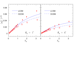
Figure 2: Variance of the smoothed convergence field $\kappa_{s}$, $\langle\kappa_{s}^{2}\rangle^{1/2}$, as a function of the source redshift $z_{s}$. The smoothing angle $\theta_{s}$ is fixed at $1$ arcminute in left panel and at $4$ arcminute in the right panel. Lines correspond to the analytical prediction (50) and data points represent results from numerical simulations (filled circles for LCDM and open circles for OCDM). Error bars are computed from scatter among various realizations.

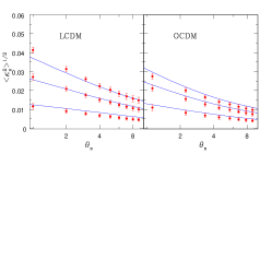
Figure 3: Variance of the smoothed convergence field $\kappa_{s}$, $\langle\kappa_{s}^{2}\rangle^{1/2}$, as a function of smoothing angle $\theta_{s}$ for three source redshifts $z_{s}$. These are $z_{s}=0.5$ (lower curve), $z_{s}=1$ (middle curve) and $z_{s}=1.5$ (upper curve). Errorbars are computed from scatter among various realizations. Different panels correspond to different cosmologies as indicated.

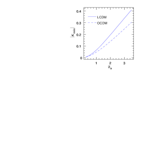
Figure 4: Minimum value $|\kappa_{\rm min}|$ of convergence $\kappa$ as a function of source redshift $z_{s}$. Note that $\kappa_{\rm min}$ is independent of smoothing angle $\theta_{s}$.

We first study here the amplitude of the smoothed convergence as a function of angle and source redshift, for both LCDM and OCDM cosmologies. Thus, we show in Fig. 2 the dependence on the source redshift $z_{s}$ of the rms convergence $\langle\kappa_{s}^{2}\rangle^{1/2}$ for two smoothing angles, $\theta_{s}=1^{\prime}$ and $\theta_{s}=4^{\prime}$. The lines show the analytical prediction (50) while the data points are the results from numerical simulations. The rms convergence increases with the source redshift, $z_{s}$, according to the (cosmology-dependent) rate of formation of structure and the location of massive structures for their gravitational lensing effects, as described by Barber et al., 2000. This makes the pdf broader. The variance is smaller for the OCDM case mainly because the normalization, $\sigma_{8}$, of the power-spectrum, $P(k)$, is smaller (see Table 1). In a similar fashion, $\langle\kappa_{s}^{2}\rangle^{1/2}$ decreases for larger smoothing angles which probe larger scales, see eq.(22), where the amplitude of the density fluctuations is smaller. We obtain a reasonable agreement with the results from numerical simulations which shows that the prescription from Peacock & Dodds (1996) is sufficient to reproduce the non-linear power-spectrum over the regime probed by these angles and source redshifts. Note indeed that eq.(50) for the variance $\xi_{\hat{\kappa}_{s}}$ only involves the Born and small-angle approximations, as well as our prescription for $P(k)$ (here taken from Peacock & Dodds, 1996).

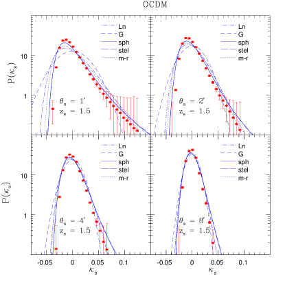
Figure 15: As for the previous Figure, but for source redshift $z_{s}=1.5$.

Next, we plot in Fig. 3 the dependence on the smoothing angle, $\theta_{s}$, of the rms convergence, $\langle\kappa_{s}^{2}\rangle^{1/2}$, for the three source redshifts, $z_{s}=0.5,1$ and $1.5$. The redshift, $z_{s}$, corresponding to the curves increases from bottom to top, in agreement with Fig. 2. Of course, as in Fig. 2 we can check that the variance grows at smaller angular scales which probe deeper within the non-linear regime of gravitational clustering. Consistently with Fig. 2 we again obtain a reasonable agreement with the results from numerical simulations, although we seem to overestimate somewhat the variance for the OCDM cosmology. However, this overestimate is within the errors associated with $N-$body simulations and the Peacock & Dodds (1996) fit to the non-linear power-spectrum. We note that the Peacock & Dodds (1996) fit underestimates the more recent simulation results of Smith et al. (2002) in the range $1<\Delta^{2}(k)<50$ for the LCDM and OCDM cosmologies, whilst it overestimates their numerical data for higher wavenumbers. Our overestimate might be due to the fact that the slope of the power, $\Delta^{2}(k)$, is somewhat steeper for OCDM (see Smith et al., 2002, Figure 15), which means that the relative contribution from high wavenumbers should be larger; whence the Peacock & Dodds (1996) fit would be expected to overestimate the simulation results by a larger amount for the OCDM cosmology than the LCDM.

Finally, we show in Fig. 4 the lower-bound $\kappa_{\rm min}$ of the convergence $\kappa$ as a function of the source redshift $z_{s}$, see eq.(5). Of course, $|\kappa_{\rm min}|$ increases at higher $z_{s}$ with the length of the line of sight. It is interesting to compare $|\kappa_{\rm min}|$ shown in Fig. 4 with the rms convergence $\langle\kappa_{s}^{2}\rangle^{1/2}$ shown in Fig. 2. Indeed, it partly describes the deviation of the pdf ${\cal P}(\kappa_{s})$ from the Gaussian. For $|\kappa_{\rm min}|\la\langle\kappa_{s}^{2}\rangle^{1/2}$ the lower-bound $\kappa_{\rm min}$ has a strong influence on the shape of the pdf which has to be significantly different from the Gaussian. On the contrary, for $|\kappa_{\rm min}|\gg\langle\kappa_{s}^{2}\rangle^{1/2}$ this lower-bound is located very far in the low convergence tail of the pdf which can therefore look roughly similar to a Gaussian (the asymmetry is weaker). Comparing Fig. 4 with Fig. 2 we see that the pdf will be more asymmetric for low source redshifts $z_{s}$. This trend also follows from the fact that low redshifts also probe the late stages of gravitational clustering where the density field has evolved farther from the Gaussian initial conditions.

6.2 The regime of gravitational clustering probed by weak-lensing

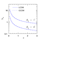
Figure 5: The typical comoving wavenumber $k_{s}$ (in units of $h$Mpc^-1) probed by the smoothed convergence $\kappa_{s}$ as a function of the redshift $z$ along the line of sight, from eq.(22). The upper pair of curves corresponds to the smoothing angle $\theta_{s}=1^{\prime}$ whereas the lower set of curves corresponds to the smoothing angle $\theta_{s}=4^{\prime}$. Note that the redshift $z$ is not the source redshift $z_{s}$ but the redshift along the line of sight ($0<z<z_{s}$) of the intermediate lensing structures.

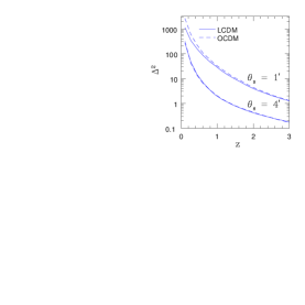
Figure 6: The power per logarithmic wavenumber interval $\Delta^{2}(k_{s}(z),z)$ as a function of redshift $z$ along the line of sight. The upper pair of curves corresponds to the smoothing angle $\theta_{s}=1^{\prime}$ while the lower set of curves corresponds to the smoothing angle $\theta_{s}=4^{\prime}$.

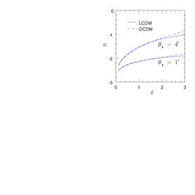
Figure 7: Spectral index $n(k_{s}(z))$ as a function of redshift $z$ along the line of sight. The upper pair of curves corresponds to the smoothing angle $\theta_{s}=1^{\prime}$ while the lower set of curves corresponds to the smoothing angle $\theta_{s}=4^{\prime}$.

As the smoothing angle $\theta_{s}$ and the source redshift $z_{s}$ vary the convergence $\kappa_{s}$ probes different scales and different regimes of gravitational clustering. This could allow one to derive some information about the physics of the gravitational dynamics in the expanding universe from future weak-lensing surveys, in addition to the measure of the main cosmological parameters.

First, because of the dependence on redshift of the angular distance ${\cal D}(z)$, eq.(4), the typical comoving wavenumber $k_{s}(z)$ probed by the smoothed convergence $\kappa_{s}$ varies with the redshift $z$ along the line of sight, see eq.(22). Thus, we display in Fig. 5 this typical comoving wavenumber $k_{s}$ as a function of $z$, for both LCDM and OCDM cosmologies and both smoothing angles $\theta_{s}=1^{\prime}$ and $\theta_{s}=4^{\prime}$. Note that the redshift $z$ is not the source redshift $z_{s}$ but the redshift along the line of sight ($0<z<z_{s}$) of the intermediate lensing structures which give rise to the deflection of the light rays. As seen from eq.(22), the wavenumber $k_{s}$ is actually proportional to $1/\theta_{s}$ as larger smoothing angles probe larger scales and smaller wavenumbers. We see that for $\theta_{s}=1^{\prime}$ the typical comoving wavenumbers probed by the convergence are of order $1$ to $10h$Mpc^-1 which corresponds to scales $0.1$ to $1h^{-1}$Mpc. These are the scales of present galaxies and clusters. In particular, this means that for such angular scales weak lensing mainly probe the intermediate regime of gravitational clustering.

This is clearly apparent in Fig. 6 which shows that the power per logarithmic wavenumber interval $\Delta^{2}(k_{s}(z),z)$ at the scales probed by weak-lensing typically runs from $\Delta^{2}(k_{s}(z),z)\sim 1$ up to $\Delta^{2}(k_{s}(z),z)\sim 400$. Note that the properties of the density field show a fast evolution in this transition regime. This entails a critical test of our simple parameterization described in Sect. 3.2, which must be able to follow the evolution of gravitational clustering from linear to highly non-linear scales. Moreover, we can suspect the mean-redshift approximation (53) to fail to reproduce the results from numerical simulations with a high accuracy in this transition range. Indeed, the value $\varphi(y;z_{*})$ of the generating function at the typical redshift $z_{*}$ may be a low-accuracy approximation to the mean (49) of the generating functions $\varphi(y;z)$ which characterize the density fluctuations encountered along the line of sight, as the latter show a significant evolution from $z=0$ up to $z=z_{s}$. This point will appear clearly in Sect. 6.3 where we discuss the skewness of the convergence shown in Fig. 9.

Finally, we show in Fig. 7 the slope $n$ of the linear power-spectrum at the scales probed by the smoothed convergence along the line of sight. We see that it runs from $n\simeq-2.5$ (for small angles and redshifts) up to $n\simeq-1$ (for large angles and redshifts). Together with Fig. 6, this shows that gravitational weak-lensing actually probes a wide range of physical conditions for the underlying density field. This requires the use of flexible models which can cover any hierarchical power-spectrum and follow the gravitational dynamics from the quasi-linear regime up to the highly non-linear regime, for arbitrary cosmological parameters. Fortunately, we shall see in the following sections that the simple model presented in Sect. 3.2, which we use in this article (except for the log-normal approximation introduced in Sect. 4.3), is able to recover the results obtained from numerical simulations with a good accuracy over all ranges of interest. On the other hand, from an observational point of view, we note that this feature makes it somewhat more difficult to derive precise constraints on the non-linear gravitational dynamics from weak-lensing surveys. Indeed, it is difficult to extract one precise scale and gravitational regime from the observed smoothed convergence $\kappa_{s}$.

6.3 The skewness $S_{3}^{\kappa_{s}}$ of the smoothed convergence

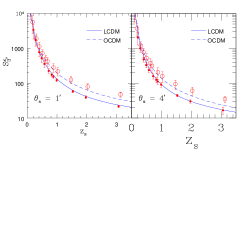
Figure 8: Skewness $S_{3}^{\kappa_{s}}$ of the smoothed convergence field $\kappa_{s}$ as a function of the source redshift $z_{s}$. The left panel corresponds to the smoothing angle $\theta_{s}=1^{\prime}$ whereas the right panel is for $\theta_{s}=4^{\prime}$. The lines show our analytical prediction (74) from the spherical-cell approximation while data points represent results from numerical simulations. Error bars are computed from the scatter among various realizations.

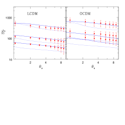
Figure 9: Skewness $S_{3}^{\kappa_{s}}$ of the smoothed convergence field $\kappa_{s}$ as a function of smoothing angle $\theta_{s}$ (in arcminute) for three source redshifts $z_{s}$. These are $z_{s}=0.5$ (upper curve), $z_{s}=1$ (middle curve) and $z_{s}=1.5$ (lower curve). Different panels correspond to different cosmologies as indicated. The solid lines show the spherical-cell approximation (74) whereas the dotted lines correspond to the mean-redshift approximation (76). The predictions from the stellar model are almost identical to spherical-cell approximation and are not reproduced here for clarity.

The simplest measure of the progress of gravitational clustering from small Gaussian initial conditions is provided by the third-order moment of the density field $\langle\delta_{R}^{3}\rangle$. As discussed in Sect. 3.1, it is actually more convenient to study the skewness $S_{3}$ defined by the ratio $S_{3}=\langle\delta_{R}^{3}\rangle/\langle\delta_{R}^{2}\rangle^{2}$, see eq.(16). Since the convergence is linear over the density field, see eq.(1), it is natural to consider also the skewness $S_{3}^{\kappa_{s}}$ of the smoothed convergence $\kappa_{s}$, defined in the same fashion. Thus, we show in Fig. 8 the dependence of $S_{3}^{\kappa_{s}}$ on the source redshift $z_{s}$. For clarity, we only plot the result from the spherical-cell approximation, which yields from eq.(48):

$$\mbox{spherical-cell}:\hskip 8.5359ptS_{3}^{\hat{\kappa}_{s}}=\frac{\langle\hat{\kappa}_{s}^{3}\rangle}{\langle\hat{\kappa}_{s}^{2}\rangle^{2}}=\frac{\int{\rm d}\chi\;\hat{w}^{3}\;S_{3}(z)\;I_{\kappa}^{2}}{\left[\int{\rm d}\chi\;\hat{w}^{2}\;I_{\kappa}\right]^{2}}$$ (74)

and:

$$S_{3}^{\kappa_{s}}=\frac{\langle\kappa_{s}^{3}\rangle}{\langle\kappa_{s}^{2}\rangle^{2}}=\frac{S_{3}^{\hat{\kappa}_{s}}}{|\kappa_{\rm min}|}.$$ (75)

We consider both LCDM and OCDM cosmologies, and the two smoothing angles $\theta_{s}=1^{\prime}$ and $\theta_{s}=4^{\prime}$. We can check in the figure that the skewness $S_{3}^{\kappa_{s}}$ decreases for larger source redshift $z_{s}$. This is partly due to the fact that higher redshifts probe earlier stages of gravitational clustering where the density field is closer to Gaussian and its skewness $S_{3}$ is also smaller. However, most of this decrease is due to the sum along the line of sight over successive mass sheets. Indeed, the total convergence $\kappa$ is the integral over the whole line of sight of the random contributions associated to the successive lens planes at redshifts $0<z<z_{s}$, see eq.(1). Then, this sum of random variables tends to make the total signal closer to Gaussian through the central limit theorem. This can also be seen as follows. Within the mean-redshift approximation (53) we have for the skewness $S_{3}^{\hat{\kappa}_{s}}$ of the normalized smoothed convergence $\hat{\kappa}_{s}$ and for $S_{3}^{\kappa_{s}}$:

$$\mbox{mean-redshift}:\hskip 5.69046ptS_{3}^{\hat{\kappa}_{s}}=S_{3}(z_{*}),\hskip 5.69046pt\mbox{and}\hskip 5.69046ptS_{3}^{\kappa_{s}}=\frac{S_{3}(z_{*})}{|\kappa_{\rm min}|}.$$ (76)

Thus, we see from eq.(76) and from the increase of $|\kappa_{\rm min}|$ with the source redshift $z_{s}$ shown in Fig. 4, that even for a constant skewness $S_{3}(z)$ for the density field we would obtain a decrease with the source redshift for the skewness $S_{3}^{\kappa_{s}}$ of the smoothed convergence (while the skewness $S_{3}^{\hat{\kappa}_{s}}$ of the normalized smoothed convergence $\hat{\kappa}_{s}$ would remain constant within the mean-redshift approximation). Of course, as noticed above, this trend is actually reinforced by the fact that higher redshifts also probe density fields which are closer to Gaussian (i.e. $S_{3}(z)$ declines at larger $z$). From the behaviour of the skewness $S_{3}^{\kappa_{s}}$ we can already infer that the pdf ${\cal P}(\kappa_{s})$ of the convergence will look closer to Gaussian for higher source redshifts.

We can see in Fig. 8 that our analytical prediction (74) shows a good agreement with the results from numerical simulations. This means that our simple parameterization (21)-(24) for the skewness of the density field provides a reasonable estimate over the range probed by weak-lensing. Indeed, the prediction obtained from the stellar model approximation is almost identical to the result computed from eq.(74) which means that the spherical-cell approximation is very good (at least for low-order moments like the skewness) and that the comparison with numerical simulations in Fig. 8 mainly tests our simple parameterization (21)-(24) for the skewness of the density field. Note the rather small dependence on $\Omega_{\Lambda}$ of the skewness $S_{3}^{\kappa_{s}}$. On the other hand, the skewness is well-known to show a strong dependence on the cosmological parameter $\Omega_{\rm m}$, which explicitly appears in $\kappa_{\rm min}$, see eq.(5). This provides a good tool to measure $\Omega_{\rm m}$ from weak-lensing surveys, see Bernardeau et al. (1997).

Next, we plot in Fig. 9 the dependence on the smoothing angle $\theta_{s}$ of the skewness $S_{3}^{\kappa_{s}}$ for the three source redshifts $z_{s}=0.5,1$ and $1.5$. In agreement with Fig. 8 the redshift $z_{s}$ corresponding to the curves increases from top down to bottom. The solid lines are the spherical-cell approximation (74) while the dotted lines are the mean-redshift approximation (76). We can see in Fig. 9 that the skewness $S_{3}^{\kappa_{s}}$ decreases for large smoothing angles $\theta_{s}$. This is due to the fact that large angles probe large scales which are closer to the linear regime, whence their skewness $S_{3}$ is smaller. This trend is also reinforced by the fact that for smaller wavenumbers $k$ the local slope $n$ of the linear power-spectrum increases (for CDM-like power-spectra like those we study here) which leads to a smaller skewness $S_{3}$ in both the linear and highly non-linear regimes, see eq.(21). We can check that our prediction (74) agrees reasonably well with the numerical simulations which shows that our simple parameterization (21)-(24) works fairly well. The results obtained from the stellar model approximation are almost identical to the solid lines which means that the spherical-cell approximation is quite good. In fact, the inaccuracy is dominated by far by the parameterization (21)-(24) rather than by the spherical-cell approximation.

On the other hand, we note that the mean-redshift approximation (76) shows some discrepancies with the simulation results. In particular, it yields a characteristic step-like profile with a sharp decrease for larger angles. This step corresponds to the transition to the highly non-linear regime where the skewness suddenly shows a sharp variation, as it evolves from $S_{3}^{\rm QL}$ up to $S_{3}^{\rm NL}$. The plateau at small angles corresponds to the highly non-linear regime where the skewness saturates, within our approximation (21), and the slope $n$ of the linear power-spectrum shows a very weak dependence on scale. Therefore, we clearly see in Fig. 9 that for smoothing angles $\theta_{s}\sim 4^{\prime}$ and source redshifts $z_{s}\sim 1$ the convergence $\kappa_{s}$ actually probes the intermediate regime of gravitational clustering, see also Fig. 6. This sharp feature does not show up in the prediction (74) given by the spherical-cell approximation because the latter involves an integration over redshift along the line of sight. This makes the prediction for $S_{3}^{\kappa_{s}}$ smoother and the decline at larger angles is shallower since it takes into account the highly non-linear scales which are still probed at low redshifts $z<z_{*}$, see also the rise at low $z$ of the typical wavenumber $k_{s}$ shown in Fig. 5. This shows that the mean-redshift approximation presented in Sect. 4.2 is not sufficiently accurate to obtain a good estimate of the skewness $S_{3}^{\kappa_{s}}$. Of course, at very small angles, where the skewness $S_{3}$ of the density field at the typical wavenumber $k_{s}(z)$ only shows a weak variation along the line of sight, as discussed above, the mean-redshift approximation becomes quite good and it recovers the result of eq.(74).

We may note that at small angles the results of numerical simulations seem to keep rising rather than to show a plateau as for the analytical predictions. This suggests that our prescription (21) is only approximate and that the skewness keeps slowly increasing within the highly non-linear regime. This corresponds to a small deviation from the stable-clustering Ansatz. Note that the latter is actually a lower bound in the sense that the skewness $S_{3}$ must either remain constant or increase in the highly non-linear regime as shown in Valageas (1999) (this only follows from the fact that the matter density is positive). An alternative to our simple parameterization (21) would be to use a halo model to evaluate $S_{3}$ within the non-linear regime. However, we shall not investigate such a model in this article since the simple parameterization (21) already provides a reasonable match to the simulation results over the range of interest, as seen in Fig. 9, and, in addition, our prescription seems to yield a better match to numerical simulations than the halo-model used in Takada & Jain (2002).

Finally, let us note that higher order moments such as the skewness take contributions from the high-$\kappa_{s}$ tail of the pdf. Hence they are more affected by the finite size of the cutoff than the variance. However we believe that for the angular scales considered in our calculations we are not limited by the size of the catalogue. We have used several realizations to probe the underlying mass distribution which provides a good handle on the errors introduced sample variance.

6.4 The pdf ${\cal P}(\kappa_{s})$ of the smoothed convergence

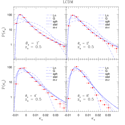
Figure 10: Probability distribution function (pdf) of the smoothed convergence $\kappa_{s}$, ${\cal P}(\kappa_{s})$, for an LCDM cosmology. Various panels correspond to various smoothing angles. The sources are fixed at a redshift $z_{s}=0.5$. Lines correspond to the analytical predictions as labeled in the Figure: spherical-cell approximation (49) (solid line), the mean-redshift approximation (53) (dotted line), the log-normal approximation (55) (dot-dash line), the stellar-model approximation (72) (dot-long dash line) and the Gaussian (dashed line). The predictions obtained from the spherical-cell approximation and the stellar-model are almost indistinguishable. Data points show the results from numerical simulations.

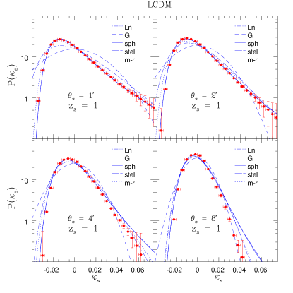
Figure 11: As for the previous Figure, but for source redshift $z_{s}=1$.

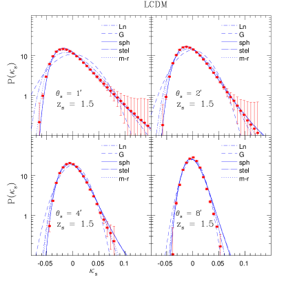
Figure 12: As for the previous Figure, but for source redshift $z_{s}=1.5$. Notice that although the variance of $\kappa_{s}$ increases with source redshift the distribution tends to become more Gaussian (see text for discussion).

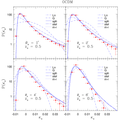
Figure 13: Probability distribution function (pdf) of the smoothed convergence $\kappa_{s}$, ${\cal P}(\kappa_{s})$, for an OCDM cosmology. Various panels correspond to various smoothing angles. The sources are fixed at a redshift $z_{s}=0.5$. Lines correspond to the analytical predictions as labeled in the Figure: spherical-cell approximation (49) (solid line), the mean-redshift approximation (53) (dotted line), the log-normal approximation (55) (dot-dash line), the stellar-model approximation (72) (dot-long dash line) and the Gaussian (dashed line). The predictions obtained from the spherical-cell approximation and the stellar-model are almost undistinguishable. Data points show the results from numerical simulations.

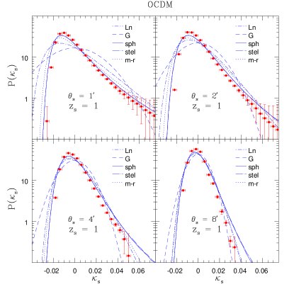
Figure 14: As for the previous Figure, but for source redshift $z_{s}=1$.

Finally, we investigate here the full probability distribution function of the smoothed convergence $\kappa_{s}$. Our analytical predictions mainly depend on our prescription for the non-linear power-spectrum, taken here from Peacock & Dodds (1996), which was specifically tested in Sect. 6.1, on our model (21)-(24) for the skewness, which was specifically tested in Sect. 6.3, and on our simple parameterization (17)-(19) for higher-order cumulants. Therefore, the shape of the pdf ${\cal P}(\kappa_{s})$ does not involve new parameters in addition to those already tested in the previous sections against numerical simulations through the variance and the skewness of the convergence. Hence the comparison with simulations of the shape of the pdf itself mainly tests the simple form (19) we used for the function $\zeta(\tau)$ (the parameter $\kappa$ being already tested through the skewness).

We compare in Figs. 10- 15 our analytical predictions against results from numerical simulations for both LCDM and OCDM cosmologies. We consider four smoothing angles, $\theta_{s}=1^{\prime},2^{\prime},4^{\prime},8^{\prime}$ and three source redshifts $z_{s}=0.5,1,1.5$. First, in agreement with Sect. 6.1 we can check that the pdf gets broader at higher $z_{s}$ as the variance increases. Second, the pdf becomes closer to a Gaussian at higher $z_{s}$, in agreement with the discussion in Sect. 6.1 and with the decrease at larger $z_{s}$ of the skewness seen in Sect. 6.3.

The various line styles correspond to the different analytical methods. Thus, we plot the spherical-cell approximation (49) (solid line), the mean-redshift approximation (53) (dotted line), the log-normal approximation (55) (dot-dash line), the stellar-model approximation (72) (dot-long dash line) and the Gaussian (dashed line). We can see that the Gaussian cannot reproduce the pdf since over these angular scales and source redshifts weak-lensing mainly probes the non-linear regime so that the pdf is already strongly asymmetric. In particular, it shows a sharp cutoff at low convergences $\kappa_{s}\ga\kappa_{\rm min}$ and an extended tail at large positive convergences, which follows the shape of the pdf ${\cal P}(\delta_{R})$ of the density contrast itself. Next, we note that although the log-normal pdf is able to exhibit a large asymmetry and provides a significant improvement over the Gaussian, it usually fails to reproduce with a reasonable accuracy the results from numerical simulations. This discrepancy is especially clear at low angles, where the variance and the skewness of the density field at scales probed by weak-lensing are large. The log-normal approximation fares better at large angles. This is due to two effects. First, the variance decreases and the pdf gets closer to the Gaussian so that any sensible approximation (like the log-normal) which goes to the Gaussian for small variance would improve in this limit. Second, larger angles probe larger scales where the slope $n$ of the linear power-spectrum increases and the skewness decreases and becomes closer to $3$. Then, as noticed in Sect. 4.3 the log-normal approximation is actually very good in the quasi-linear regime for $n\simeq-1$ and $S_{3}\simeq 3$ (it also coincides with our parameterization (17)-(19) in this limit). This explains why the log-normal pdf works better at large angles $\theta_{s}\sim 8^{\prime}$.

On the other hand, we can see that our analytical predictions based on the simple parameterization described in Sect. 3.2 show a reasonably good agreement with numerical simulations over all angular scales and source redshifts. The improvement over the log-normal pdf is not surprising since the model (19)-(24) allows us to follow the dependence on time and scale of the skewness $S_{3}$ of the density field for any slope $n$ of the linear power-spectrum. This was already specifically tested in Sect. 6.3. Then, Figs. 10- 15 show that the simple form (19) for the function $\zeta(\tau)$ which implicitly determines the higher-order moments of the density field provides a reasonable prescription. In fact, the agreement with numerical simulations is surprisingly good in view of the simplicity of the model (19)-(24). At large angles our prescription seems to overestimate the large-$\kappa_{s}$ tail of the pdf. This might be cured by using for the function $\zeta(\tau)$ the exact result derived for the quasi-linear regime (Bernardeau, 1994, Valageas, 2002), or our simple interpolation (24) may overestimate the skewness in the transition regime, although this does not seem to be the case for the OCDM cosmology, see Fig. 9. However, since the high-$\kappa_{s}$ tail of the pdf for large angles $\theta\ga 8^{\prime}$ may not be of great practical interest we shall not try in this article to improve over the model (19)-(24) which shows the advantage of a great simplicity.

From Figs. 10- 15, we note that all approximations based on the simple parameterization (19)-(24) yield very close predictions. They only show some small differences in the far tail of the pdf, at large positive $\kappa_{s}$, which is very sensitive to the details of the model. In particular, the agreement between the spherical-cell prediction (49) (solid line) and the stellar-model prediction (72) (dot-long dash line) shows that the spherical-cell approximation (45) is very accurate and it is sufficient to derive the pdf of the smoothed convergence ${\cal P}(\kappa_{s})$. Therefore, it is not necessary to know the detailed behaviour of the many-body correlations $\xi_{p}$: the knowledge of the cumulants $\langle\delta_{R}^{p}\rangle_{c}$ over spherical cells is largely sufficient to predict with a very high accuracy the pdf ${\cal P}(\kappa_{s})$ of the smoothed convergence $\kappa_{s}$. This is an important point since it shows that the measure of the pdf ${\cal P}(\kappa_{s})$ would provide a very robust estimate of the pdf ${\cal P}(\delta_{R})$, with no degeneracy with the detailed angular dependence of the many-body correlations (e.g., whether they are described by a minimal tree-model or a stellar-model).

Eventually, let us note that the numerical computation of the pdf from simulation maps suffers from various systematics. For a finite size catalogue, clearly the high-$\kappa_{s}$ tail cannot continue to infinity. In general the high-$\kappa_{s}$ tail shows large fluctuations due to the presence (or the absence) of rare overdense (underdense) objects before showing an abrupt cutoff. Such effects have been studied in great detail for galaxy catalogues (see e.g. Bernardeau et al. 2002) as well as for weak lensing surveys (Munshi & Coles 2003). A comparison of our numerical results with larger simulation volumes will help us to quantify such systematic deviations.

7 Discussion

Ongoing weak lensing surveys with wide field CCD imaging are being used to produce shear maps for areas of order 10 square degrees. Soon, larger patches, $10^{\circ}\times 10^{\circ}$, will also be feasible, e.g., from various surveys including the MEGACAM camera on the Canada-France-Hawaii Telescope and the VLT-Survey Telescope. Such surveys will provide a very interesting insight into the dynamics of the universe and the clustering in the mass distribution on small angular scales, where the density distribution is highly non-linear. They will provide opportunities to test our knowledge of gravitational clustering at small length scales where no rigorous analytical results are presently available. Indeed, unlike galaxy surveys, weak lensing surveys provide an unbiased picture of matter clustering, as they directly probe the gravitational potential. Results from such future surveys will be especially useful where they provide additional data in the form of photometric redshift information based on the multi-colour data. In these cases the additional radial information may assist in building up a three-dimensional picture of the dark matter structure.

Statistics of the convergence, $\kappa_{s}$, can not only be studied from the by-product of shear maps generated from weak lensing surveys, but can also be studied from the magnification effects of clustered matter which produce variations in the image sizes and number density of galaxies across the sky (see, e.g., Jain, 2002). Although there are considerable difficulties in practice in using these effects, as described at length by Bartelmann & Schneider (2001), use of such results from wide field surveys can map the large-scale structure and help us to quantify its statistics. Recent order-of-magnitude analysis of the signal-to-noise ratio as a function of angular scale and source redshift have suggested that well-designed forthcoming surveys will have high signal-to-noise ratios on scales of about 0.1 arcminute to several degrees. This will help us to probe the clustering of matter on spatial scales of about 50 kpc to 100 Mpc.

Recent studies of weak lensing have focussed mainly on recovering the mass power-spectrum, either from weak lensing data alone or from joint analyses of CMB and weak lensing surveys (see e.g., Contaldi et al., 2003, for recent estimates). Although such joint analyses can pinpoint the cosmological parameters very effectively, the non-Gaussianities we study here form a complementary approach and are able to break the degeneracies in estimating the cosmological parameters from weak lensing surveys alone.

Most previous analytical studies of weak lensing statistics can be divided in two categories. A majority of previous works has used a perturbative analysis (Bernardeau et al. 1997) which is only applicable in the quasi-linear regime and hence will require a large smoothing angle. Although interesting however, such studies will have limited use for currently ongoing surveys as survey areas of order 10 square degrees are necessary to validate such smoothing angles while still keeping effects of finite size of the survey area low on various statistical quantities. However, given that existing CCD cameras typically have diameters of $0.25^{\circ}-0.5^{\circ}$, the current weak lensing surveys are providing us statistical information on small smoothing angles, of order $10^{\prime}$ and less.

Therefore, some earlier studies have also investigated the non-linear regime using a hierarchical Ansatz to compute weak lensing statistics on smaller angular scales (e.g. Valageas 2000a,b, Munshi & Jain 2000, Munshi 2000). It was shown that the hierarchical ansatz when combined with extensions of perturbative calculations such as Hyper-extended perturbation theory can provide an accurate picture of weak lensing statistics on highly nonlinear scales. In this paper we extend these predictions to check their validity by comparing analytical predictions with results from numerical simulations over a large range of angular scales and redshifts. Thus, we have presented two model-independent approximations which allow one to obtain the pdf of the convergence (and all its moments). The first method, the “spherical-cell approximation”, simply assumes that the relative amplitude of the many-body density correlations smoothed at a given scale shows a weak dependence on the shape of the real-space filter, while the second one, the “mean-redshift approximation”, makes the further approximation that the properties of the density field along the line-of-sight can be estimated by considering a typical intermediate redshift. Next, we have evaluated the accuracy of these approximations by considering a specific “stellar model” for the many-body density correlations where exact calculations can be performed. We find that in this case the spherical-cell approximation is actually very good and can barely be distinguished from the exact result. This shows that the smoothed convergence $\kappa_{s}$ is a very robust tool to measure the statistics of the density fluctuations at a given scale and it does not depend on the detailed angular behaviour of the many-body density correlations (it only involves their overall amplitude at this scale). On the other hand, we find that the “mean-redshift approximation” provides a reasonable prediction, in agreement with previous works (Valageas 2000b), but it does not give a very accurate prediction for the low-order cumulants like the skewness at intermediate angular scales, as the properties of the density field show significant variations along the line-of-sight as it evolves from the linear to the highly non-linear regime. A simple model which has been proposed to describe the density field from linear to non-linear scales is the log-normal approximation. We have applied this model to the derivation of the pdf of the convergence based on the mean-redshift approximation. Then, we find that while the log-normal approximation may be a good description for smoothing angles $\theta_{s}>4^{\prime}$ it is not sufficiently accurate for smaller scales. This is related to the facts that such scales are deeper in the non-linear regime and the local slope $n$ of the linear power-spectrum $P(k)$ is significantly different from $-1$, so that the log-normal approximation underestimates the skewness. Finally, we have applied the three general methods described above (i.e., the spherical-cell, mean-redshift and stellar-model approximations) to a very simple model for the evolution of the density fluctuations from the linear to the highly non-linear regime. We find a good agreement with the results from numerical simulations for a wide range of source redshifts as well as smoothing angles, for both LCDM and OCDM cosmologies.

An alternative approach to model non-linearities in gravitational clustering which has emerged in recent years is the “Halo model” (see e.g. Cooray A. & Sheth R for a recent review). In this approach the dark matter is modeled as belonging to halos with a mass function given by the Press-Schechter formalism and a spatial distribution modeled as in Mo & White (1996) or its variants. When supplemented by a radial profile for the dark halos such a prescription can be used to compute many statistical quantities associated with the density field. These models have also been applied to model statistics of the convergence field. Our approach is complimentary to such methods. It is better-suited to the study of weak-gravitational lensing effects which directly probe the density field (and its many-body correlations) and do not involve the decomposition of the universe over various classes of objects and virialized halos. In this sense, our approach is more natural and the measures obtained from weak-lensing surveys (e.g., the low-order moments of the convergence or the shear) are directly related to the density correlations which are the basic ingredients of our methods. On the other hand, halo models can provide an interesting connection between weak-lensing effects and the properties of virialized halos (so that one might hope to derive for instance some constraints on the profiles of these halos). However, in our opinion, it is not clear, until fully tested, that they can provide a full description of weak-lensing effects which also probe low-density regions located outside of virialized objects.

In our studies, both analytical and numerical, we find that lower order moments are rather sensitive to the source redshift. In this article we only considered the case where all sources are located at the same redshift $z_{s}$ but it is straightforward to apply our analytical methods to more realistic broad distributions of source redshifts. We plan to investigate this point in future studies when relevant numerical simulations are available. In agreement with previous results we found that while the variance of convergence field (independently of smoothing angle) increases with the depth of the survey, the distribution of $\kappa_{s}$ tends to become more Gaussian, thereby reducing the values of the $S_{p}^{\kappa_{s}}$ parameters. Nevertheless, the ordering of the $S_{p}^{\kappa_{s}}$ parameters in two different cosmologies does not change with source redshifts. For any given source redshift the $S_{3}^{\kappa_{s}}$ parameter is higher in the OCDM scenario as compared to the LCDM cosmology. The $S_{p}^{\kappa_{s}}$ parameters show a rapid increase at small redshifts whereas at large redshifts they vary at a much slower rate. Of course, perturbative analysis of the dependence of the $S_{p}^{\kappa_{s}}$ parameters on source redshift gives a qualitatively similar dependence.

Although we have not taken into account the effect of the finite size of the catalogue, it is unlikely to have any effect on the length scales we have probed in our studies. However, the finite size is likely to play an important role in the determination of the cosmological parameters. It is therefore of interest to incorporate such effects in future simulations. The effects on lower order moments have been studied analytically by Munshi & Coles (2003) and we note that the higher-order, $S_{p}$, parameters enter in the expressions for the computation of errors for the lower-order moments associated with the convergence.

Noise due to the intrinsic ellipticities of lensed galaxies will also need to be modeled. Our analytical results provide a strong foundation for such studies and we plan to include such features in our future work. The intrinsic ellipticity distribution of galaxies can be modeled by assuming a Gaussian distribution, which depends only on a knowledge of the variance in the distribution. To compute the noisy pdf it is therefore necessary to convolve the theoretical convergence pdf with the noise pdf to produce a resultant containing information on both the underlying mass distribution and the noise. Initial studies in this direction have been attempted by Van Waerbeke (2000) and Jain & Van Waerbeke (1999).

All analytical calculations regarding weak lensing statistics rely on the so called Born approximation (Schneider et al. 1998). However, its validity at non-linear scales is difficult to establish by analytical calculations alone. While a weakly clustered dark matter distribution is expected to produce small deflections of photon trajectories, it is not clear whether the small-angle approximation can be safely used at small angular scales which probe large density fluctuations. However, the agreement of our analytical predictions with numerical simulations strongly suggests that the Born approximation can be used down to $\theta_{s}=0.4^{\prime}$ at least and that cases of large deflections of photon trajectories definitely have a small statistical significance even on these small angular scales. In fact, the theoretical uncertainty is dominated by the inaccuracy of the simple models used for the non-linear evolution of the density field.

Finally, let us note that our simulations are different from more popular ones based on ray-tracing techniques and are based on computations of the 3-dimensional shear along the lines of sight. The comparison of analytical and numerical results for convergence maps are complementary to similar analysis of shear maps presented in Valageas, Barber & Munshi (2003). The excellent match between analytical and simulation results in both cases increases our faith in both the analytical and numerical methods.

References

- [1] Babul A., Lee M.H., 1991, MNRAS, 250, 407
- [2] Barber A. J., MNRAS, 2002, 335, 909
- [3] Barber A. J., Taylor A. N., 2002, submitted to MNRAS, (astro-ph/0212378)
- [4] Barber A. J., Thomas P. A., Couchman H. M. P. & Fluke C. J., 2000, MNRAS, 319, 267
- [5] Balian R., Schaeffer R., 1989, A&A, 220, 1
- [6] Bartelmann M., Schneider P., 2001, Physics Reports, 340, 291B
- [7] Bernardeau F., 1992, ApJ, 392, 1
- [8] Bernardeau F., 1994, A&A, 291, 697
- [9] Bernardeau F., Schaeffer R., 1992, A&A, 255, 1
- [10] Bernardeau F., Valageas P., 2000, A&A, 364, 1
- [11] Bernardeau F., Van Waerbeke L., Mellier Y., 1997, A&A, 322, 1
- [12] Bernardeau F., Mellier Y., Van Waerbeke L., 2002, A&A, 389, L28
- [13] Bernardeau F., Colombi S., Gaztanaga E., Scoccimarro R., Phys.Rept., (2002), 367, 1
- [14] Blandford R.D., Saust A.B., Brainerd T.G., Villumsen J.V., 1991, MNRAS, 251, 600
- [15] Boschan P., Szapudi I., Szalay A.S., 1994, ApJS, 93, 65
- [16] Colombi S., Bouchet F.R., Schaeffer R., 1995 ApJS, 96, 401
- [17] Colombi S., Bouchet F. R., Hernquist L., 1996, ApJ, 465, 14
- [18] Couchman H. M. P., Barber A. J., Thomas P. A., 1999, MNRAS, 308, 180
- [19] Couchman H. M. P., Thomas P. A., Pearce F. R., 1995, Ap. J., 452,
- [20] Cooray A., Sheth R., Phys.Rept. 372 (2002) 1, 797
- [21] Davis M., Peebles P.J.E., 1977, ApJS, 34, 425
- [22] Fry J.N., 1984, ApJ, 279, 499
- [23] Fry J.N., Peebles P.J.E., 1978, ApJ, 221, 19
- [24] Groth E., Peebles P.J.E., 1977, ApJ, 217, 385
- [25] Gunn J.E., 1967, ApJ, 147, 61
- [26] Hamilton A.J.S., Kumar P., Lu E., Matthews A., 1991, ApJ, 374, L1
- [27] Hoekstra H., Yee H. K. C., Gladders M. D., 2002, ApJ, 577, 595
- [28] Hui L., 1999, ApJ, 519, 622
- [29] Jain B, 2002, ApJ., 580, L3
- [30] Jain B., Mo H.J., White S.D.M., 1995, MNRAS, 276, L25
- [31] Jain B., Seljak U., 1997, ApJ, 484, 560
- [32] Jain B., Van Waerbeke L., 1999, astro-ph/9910459
- [33] Jannink G., Des Cloiseaux J., 1987, Les polymères en solution, Les editions de physique, Les Ulis, France 1990, ApJ, 365, 22
- [34] Jaroszyn’ski M., 1991, MNRAS, 249, 430
- [35] Kaiser N., 1992, ApJ, 388, 272
- [36] Kaiser N., 1998, ApJ, 498, 26
- [37] Limber D.N., 1954, ApJ, 119, 665
- [38] Lee M.H., Paczyn’ski B., 1990, ApJ, 357, 32
- [39] Masahiro T., Jain B., 2003, ApJ, 583, L49
- [40] Miralda-Escudé J., 1991, ApJ, 380, 1
- [41] Munshi D., Bernardeau F., Melott A.L., Schaeffer R., 1999, MNRAS, 303, 433
- [42] Munshi D., Coles P., Melott A.L., 1999a, MNRAS, 307, 387
- [43] Munshi D., Coles P., Melott A.L., 1999b, MNRAS, 310, 892
- [44] Munshi D., Melott A.L., Coles P., 1999, MNRAS, 311, 149
- [45] Munshi D., Coles P., 2000, MNRAS, 313, 148
- [46] Munshi D., Coles P., 2002, MNRAS.329, 797
- [47] Munshi D., Coles P., 2003, MNRAS, 338, 846
- [48] Munshi D., Jain B., 2000, MNRAS, 318, 109
- [49] Munshi D., Jain B., 2001, MNRAS, 322, 107
- [50] Munshi D., 2000, MNRAS, 318, 145
- [51] Munshi D., Wang Y., 2003, ApJ, 583, 566
- [52] Navarro J.F., Frenk C.S., White S.D.M., 1996, ApJ, 462, 563
- [53] Peebles P.J.E., 1980, The large scale structure of the universe, Princeton University Press
- [54] Peacock J.A., Dodds S.J., 1996, MNRAS, 280, L19
- [55] Peacock J. A., Smith R. E., 2000, MNRAS, 318, 1144
- [56] Pen U.-L., et al., 2003, accepted by ApJ, (astro-ph/0302031)
- [57] Premadi P., Martel H., Matzner R., 1998, ApJ, 493, 10
- [58] Schaeffer R., 1984, A&A, 134, L15
- [59] Schneider P., Ehlers J., Falco E. E., 1992, ‘Gravitational Lenses,’ Springer-Verlag, ISBN 0-387-97070-3
- [60] Schneider P., Lombardi M., 2003, A&A, 397, 809
- [61] Schneider P., Van Waerbeke L., Jain B., Kruse G., 1998, MNRAS, 296, 873, 873
- [62] Scoccimarro R., Colombi S., Fry J.N., Frieman J.A., Hivon E., Melott A.L., 1998, ApJ, 496, 586
- [63] Scoccimarro R., Frieman J.A., 1999, ApJ, 520, 35
- [64] Scoccimarro R., Zaldarriaga M., 2003, ApJ, 584, 559
- [65] Seljak U., 2000, MNRAS, 318, 203
- [66] Smith R. E., Peacock J. A., Jenkins A., White S. D. M., Frenk C. S., Pearce F. R., Thomas P. A., Efstathiou G., Couchman H. M. P, 2002, astro-ph/0207664
- [67] Stebbins A., 1996, astro-ph/9609149
- [68] Szapudi I., Szalay A.S., 1993, ApJ, 408, 43
- [69] Szapudi I., Szalay A.S., 1997, ApJ, 481, L1
- [70] Takada M., Jain B. 2002, MNRAS 337, 875
- [71] Taruya A., Takada M., Hamana T., Kayo I., Futamase T., 2002, ApJ, 571, 638
- [72] Valageas P., 1999, A&A, 347, 757
- [73] Valageas P., 2000a, A&A, 354, 767
- [74] Valageas P., 2000b, A&A, 356, 771
- [75] Valageas P., 2002, A&A, 382, 412
- [76] Valageas P., Schaeffer R., 1997, A&A, 328, 435
- [77] Valageas P., Barber A. J., Munshi D., 2003, submitted to MNRAS, (astro-ph/0303472)
- [78] Van Waerbeke L., 2000, MNRAS, 313, 524
- [79] Van Waerbeke L., Bernardeau F., Mellier Y., 1999, A& A, 342, 15
- [80] Van Waerbeke L., Hamana T., Scoccimarro R., Colombi S., Bernardeau F., 2001, MNRAS, 322, 918 H. J., Jain B., 2002, A&A, 393, 369
- [81] Villumsen J.V., 1996, MNRAS, 281, 369 298
- [82] Wambsganss J., Cen R., Xu G., Ostriker J.P., 1997, ApJ, 494, 29
- [83] Wambsganss J., Cen R., Ostriker J.P., Turner E.L., 1995, Science, 268, 274
- [84] Wang Y., Holz D. E., Munshi D., 2002, ApJ, 572L, 15
- [85] White M., Hu W., 2000, ApJ, 537, 1
- [86] Zaldarriaga M., Scoccimarro R., 2003 ApJ, 584, 559