Disentangling microlensing and differential extinction in the
double QSO HE~0512–3329

We present the first separate spectra of both components of the small-separation double QSO HE~0512–3329 obtained with HST/STIS in the optical and near UV. The similarities especially of the emission line profiles and redshifts strongly suggest that this system really consists of two lensed images of one and the same source.

The emission line flux ratios are assumed to be unaffected by microlensing and are used to study the differential extinction effects caused by the lensing galaxy. Fits of empirical laws show that the extinction properties seem to be different on both lines of sight. With our new results, HE~0512–3329 becomes one of the few extragalactic systems which show the 2175 Å absorption feature, although the detection is only marginal.

We then correct the continuum flux ratio for extinction to obtain the differential microlensing signal. Since this may still be significantly affected by variability and time-delay effects, no detailled analysis of the microlensing is possible at the moment.

This is the first time that differential extinction and microlensing could be separated unambiguously. We show that, at least in HE~0512–3329, both effects contribute significantly to the spectral differences and one cannot be analysed without taking into account the other. For lens modelling purposes, the flux ratios can only be used after correcting for both effects.

1 Introduction

HE~0512–3329 was discovered as a probable lensed quasar in the course of a snapshot survey with the Space Telescope Imaging Spectrograph (STIS). It is a doubly imaged QSO with a source redshift of $z=1.58$ and an image separation of $0\aas@@fstack{\prime\prime}644$. The lensing galaxy has not been detected yet, but strong metal absorption lines with a redshift of $z=0.93$ identified in the integrated spectrum provide good evidence that a damped Ly$\alpha$ (DLA) system intervenes at this redshift. This system is very probably associated with the lensing galaxy (Gregg et al. 2000).

The absorption lines provide the possibility to study the interstellar matter (ISM) of the lensing galaxy along the two lines of sight, separated by 5.1 kpc at the proposed lens redshift, which allows us to learn more about the nature of the DLA absorber by comparing column densities of hydrogen and metals as well as kinematic profiles along both lines of sight. HE~0512–3329 is especially well suited for such investigations because of the wealth of absorption features and the close image separation.

The propagation effects of microlensing and extinction in the lensing galaxy can be studied by using the fact that we see two images of the same source. In singly imaged sources, it is not possible to uniquely identify microlensing or extinction effects because the true source fluxes and spectra are not a priori known. In the case of multiply imaged sources, this problem can be circumvented by using only differences of the individual images as diagnostic. These differences are independent of the true source spectrum and flux and therefore allow the examination of differential propagation effects.

An additional complication arises from possible variability of the source. Because of the time-delay, observations of both components taken at the same time are really snapshots of the source at different epochs. To correct for this effect (which is thought to be negligible for the emission lines because of the longer variability time scale), (spectro)photometric monitoring is necessary to determine the time-delay and obtain measurements at the same source epoch.

It has been known from earlier photometric observations that the flux ratio A$/$B in HE~0512–3329 shows a strong dependence on wavelength. In the $R$ and $I$ bands, A is brighter than B by about 0.45 mag while the two are almost equal in $B$ (Gregg et al. 2000). A natural explanation for this effect is differential reddening caused by different extinction effects in the two lines of sight. This scenario is supported by the strong metal lines already visible in the integrated spectrum of HE~0512–3329 (Gregg et al. 2000) which make the existence of significant amounts of dust very likely. Under this assumption, Gregg et al. (2000) estimated a relative visual extinction of $A_{V}=0.34\,\mathrm{mag}$ by fitting galactic extinction curves with $R_{V}=E(B-V)/A_{V}=3.1$ on both lines of sight to the photometric data. We will see later that this approach is not appropriate in the case of HE~0512–3329.

The other possible explanation is microlensing by stars and other compact objects in the lensing galaxy. Since the lines of sight cross different star fields in the lens, the microlensing effect is independent for A and B and can be observed in the difference. The lensing effect itself is an achromatic process, but chromatic effects are nevertheless expected if different parts of the source, which are influenced by different microlensing amplifications, have different colours. Since the microlensing amplification pattern has a high contrast on very small scales, the effectively observed total amplification of the integrated source depends significantly on the size of the source. The effect is maximal for point sources but is smoothed out and thus reduced for larger sources.

Standard models of QSOs consist of different emitting regions of very different sizes (see e.g. Krolik 1999). Smallest is the continuum region, which itself scales with wavelength. Broad line regions are expected to be much larger than the continuum region but smaller than the narrow line regions. The whole range of scale lengths covers several orders of magnitude. This means that the microlensing signal should be strongest for the continuum, only very weak at most for the broad emission lines and absent for narrow lines.

This size-dependent behaviour of microlensing gives a possible clue to separate the effect from differential extinction and study the two processes separately. Microlensing is smeared out in the emission lines whose fluxes are thus only influenced by the differential extinction. The continuum, on the other hand, is also affected by microlensing. The extinction itself is a smooth function of wavelength but does not depend on the source size. We can therefore use the emission lines to study the extinction directly without worrying about microlensing and correct the continuum for extinction to study the pure differential microlensing in the remaining differences.

The spectra we use to follow this approach were obtained with STIS on board the HST in the optical and near UV covering the QSO emission lines of Ly $\beta$, Ly $\alpha$, Si iv, C iv and C iii] with the goal to study the differential extinction by comparing the continua of the A and B images.

The results of these observations are presented in this paper. We show the first separate spectra of the A and B images and use the similarity of these to confirm the nature of the object as a gravitational lens system. We use the combination of continuum and emission lines to disentangle the effects of extinction and microlensing as described above. We see that microlensing actually does influence the flux ratio significantly and that the continuum cannot be used to study the extinction directly.

To analyse the differential extinction we will fit empirical extinction laws to our emission line data and discuss the results. The microlensing data will be used to estimate an upper limit of the source size using the assumption that variability and time-delay effects can be neglected.

This is the first time that such a detailed attempt to separate the effects of differential extinction and microlensing has been successfully performed for any lens system.

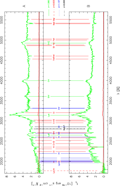
Figure 1: The combined spectra of HE~0512–3329, smoothed with a Gaussian filter of FWHM=$3.5$ Å. Component A is at top, B at bottom. The curve near $f_{\lambda}=0$ shows the statistical errors. The middle panel marks emission and absorption features at $z=1.58$ (QSO emission), $z=0.933$ (DLA system), $z=1.137$ (Lyman limit system) and $z=0$ (galactic absorption).

2 Observations and initial data reduction

To cover a sufficiently large spectral range, we used the CCD for the optical and the near UV MAMA detector for the UV part. The slit was positioned along the line connecting the two QSO components.

The CCD spectra were taken on 13 August 2001 with the G430L grating and 52x0.5 aperture, covering a spectral range from 2900 to $5700\,\mbox{\AA}$ (Leitherer et al. 2001). With a spectral element size of $2.73\,\mbox{\AA}$, the resolution is about $3.8\,\mbox{\AA}$. Three exposures with total integration time of 2266 sec and a standard dithering pattern were used.

Data reduction started with a standard 2-dimensional reduction including flat-fielding, flux and wavelength calibration with the CALSTIS software Version 2.10 (Brown et al. 2002) in IRAF V2.12 with STSDAS Version 2.3. Cosmic ray rejection could not be performed in a standard way because the individual exposures were not done in CR-SPLIT mode. We therefore used our own software, developed specifically for this task, to apply the shifts, reject cosmic ray events and combine the images.

We then used the CALSTIS task X1D to extract the spectra of both QSO components separately. A smaller than standard extraction width was used to minimize the fraction of measurements being rejected due to flagged bad pixels or cosmic rays.

The three resulting extracted spectra were finally combined and cleaned of still remaining cosmic rays and otherwise deviant pixels with our own software.

The MAMA spectra were taken with the G230L grating and 52x0.2 aperture, covering a range from 1570 to $3180\,\mbox{\AA}$ with an element size of $1.58\,\mbox{\AA}$ and a resolution of $3.3\,\mbox{\AA}$. The six exposures of a total of 16588 sec were taken on 15 August 2001, only two days after the CCD spectra. Since the MAMA detector is not sensitive to cosmics, a standard CALSTIS reduction could be used to calibrate the 2-dimensional images. To extract the two QSO components separately, X1D was used with a slightly smaller than standard extraction width and with background regions adapted to the situation of two closely separated but well resolved spectra. The six MAMA spectra were then combined with the same algorithm as the CCD spectra.

For the analysis, we did not use the short wavelength end of the combined CCD spectrum ($<3020\,\mbox{\AA}$) and the long wavelength end of the MAMA spectrum ($>3120\,\mbox{\AA}$). In these regions, the $S/N$ is not optimal and calibration uncertainties are expected to be worst. In the remaining overlapping region, the two spectra agree very well and a simple averaging combination was used for the final spectrum.

The typical error per spectral element of the final combined spectrum is 1–$2\cdot 10^{-17}\,\mathrm{erg\,s^{-1}\,cm^{-2}\,\mbox{\AA}{}^{-1}}$, except near $\lambda\approx 3100\,\mbox{\AA}$ and for $\lambda<1700\,\mbox{\AA}$. This is equivalent to a $S/N$ of 30 per element in the optical and about 15 in the UV region.

3 The spectra

3.1 First view

Figure 1 shows the combined spectra from all CCD and MAMA exposures. These comprise the first separate spectra of the two QSO components in HE~0512–3329. The general features of A and B look very similar. The relative strength of the emission lines, their profiles (see also Fig. 4 and discussion below) and redshifts agree very well which strongly confirms the interpretation as two lensed images of one source. The continua, on the other hand, show similarities as well as significant differences which will be discussed in detail in the later parts of this paper.

The wealth of absorption features seen in both images can provide important information about column densities of both hydrogen and metals and will be discussed in detail in another publication. The spectra confirm the existence of a DLA system at a redshift of $z=0.933$ which was already proposed by Gregg et al. (2000) to explain the strong low-ionization metal lines in the (then still combined A+B) spectrum. Our estimate of the redshift differs only slightly from the former measurement by Gregg et al. (2000) of $z=0.9313\pm 0.0005$. Figure 1 identifies the anticipated DLA line as well as a high number of metal absorption features at the same redshift in both components. The break at about $2000\,\mbox{\AA}$, which is especially prominent in B due to the higher continuum there, does not correspond to this already known system at $z=0.93$ but is caused by a second intervening Lyman limit system at a redshift of about $z=1.137$. This system is much weaker than the lower redshift one but nevertheless shows some metal lines which are also identified in Fig. 1. Weak Mg ii absorption at a very similar redshift ($z=1.1346$) was already noticed by Gregg et al. (2000). Finally we detect galactic Mg i+ii absorption at a redshift consistent with zero.

A quantitative analysis of the absorption features, combined with high resolution UVES spectra, will be published in an upcoming paper (Lopez et al., in prep.). Especially important is the analysis of the DLA lines in our spectra which provide the H i column density needed to determine metalicities in both lines of sight.

3.2 Differences in the global shape of A and B

Although the two spectra have many features in common, there are some highly significant differences. Most prominent is the very different behaviour of the continuum flux on large wavelength scales. On the red side of $\lambda\approx 4600\,\mbox{\AA}$, the A component is brighter than B. For smaller wavelengths, especially close to the limit near 2000 Å, B becomes much brighter than A. This effect has already been described by Gregg et al. (2000) using photometric data in $B$, $V$, $R$ and $I$. While A is brighter by about 0.45 mag in $I$ and $R$, the difference starts to decrease in $V$ and is compatible with zero in the $B$ band.

Given the similarities of the spectra, the differences have to be interpreted in a lensing context. As discussed in the introduction, two possible explanations will be discussed here. One is differential reddening by different amounts of dust along both lines of sight in the lensing galaxy, the other is microlensing which by different amplification patterns for the two images in combination with a colour gradient of the source can also result in chromatic effects.

To separate these effects, we use the assumption that the regions causing the emission lines are much larger than the continuum region so that the microlensing signal is smeared out in the emission lines. We can thus use the emission lines to study the pure extinction signal. In the next step we correct the continuum (which is affected by extinction and microlensing) for extinction to study the microlensing effect. To accomplish these tasks, we have to fit the continuum and determine the flux ratios of the continuum-subtracted emission lines.

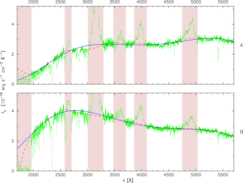
Figure 2: Observed spectrum of A (top) and B (bottom) together with the two different continuum fits. The global polynomial fit is shown solid, the locally smoothed estimate is dashed. The shaded regions mark the emission lines and the region affected by the Lyman limit on the far left. Parts of the spectra not included in the fit (in the emission line regions or rejected by the global polynomial fitting algorithm because of low flux) are shown dotted, the rest of the spectra is solid.

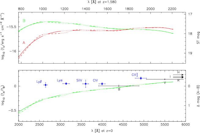
Figure 3: Top: Continuum flux of A and B. Bottom: Flux ratio $\mathrm{A}/\mathrm{B}$ (curve). The error crosses above the lines are for the continuum subtracted emission lines, where the horizontal bar shows the FWHM of the lines. Photometric measurements (combined continuum and emission lines) are shown at the right (see text). The photometric error bars are formal statistical uncertainties. $R$, $I$ and $H$ are outside of the wavelength range and are shown as arrows. The same line type coding as in Fig. 2 is used for the continuum fits in both panels. The regions of emission lines were not used for the fits and are shown dotted.

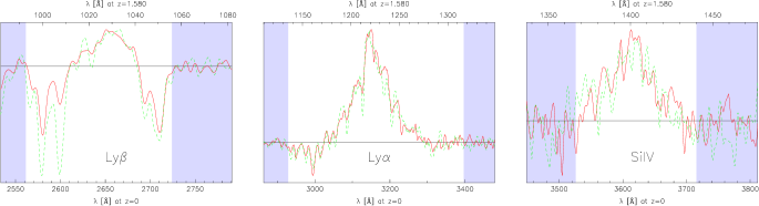
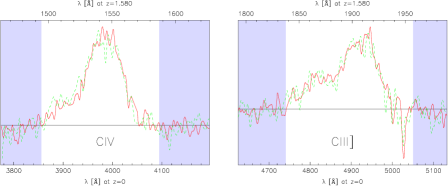
Figure 4: Profiles of the five emission lines after local continuum subtraction. A is plotted solid, B is dashed. The flux of B was scaled by the determined emission line flux ratio to obtain the same level for both components. The shaded regions were used for the linear continuum fit with rejection of absorption features. The spectra are smoothed with a Gaussian kernel of FWHM=5 Å.

3.3 Global continuum fit

We first flagged the regions of the five strong emission lines of both spectra and kept only the continuum which is still covered with many absorption lines. We tried two approaches to fit the global continuum. One is a global fit of a polynomial of degree 4 to the logarithmic flux. The other is a smoothing algorithm which works by fitting a quadratic function to the spectrum for each wavelength, using a Gaussian weighting with FWHM of 300 Å to effectively include only nearby data points. The central value of this local fit is taken as the result for the central wavelength and the procedure is repeated for each wavelength. This algorithm is more appropriate than a simple Gaussian convolution filter because it can follow local slopes and curvatures more accurately. In particular it avoids any edge effects. In both algorithms we allowed for a certain fraction of pixels to deviate in a negative direction from the model to avoid absorption lines affecting the fit. These pixels were then discarded in the $\chi^{2}$ summation. We started with this fraction set to zero and then increased it slowly until a level of 30 % was reached. This value was chosen to obtain a final normalized $\chi^{2}$ close to unity. It is equivalent to a final effective (one-sided) clipping limit of about 1.5–$1.7\,\sigma$.

The global continuum fits are shown in Fig. 2 together with the observed spectrum. In the comparison, the locally smoothed continuum follows the spectrum more closely while the global polynomial fit is slightly smoother on large scales. Both curves look like good continuum fits to the eye, and the small differences are not significant for the further analysis which was performed with both fits. We have to keep in mind, however, that the continuum short-wards of the Ly $\beta$ emission line might still be significantly contaminated by the Lyman forest. This should not be a problem in the continuum subtraction of the emission line, because the broad emission lines are affected by the Lyman forest as well. The shape of the continuum near the short wavelength end itself should nevertheless be interpreted with caution. Figure 3 shows the continuum of A and B (top) as well as the ratio of the two (bottom) as a function of $\lambda$.

3.4 Emission line fluxes

The main problem in calculating the emission line fluxes is the continuum subtraction. We used three different estimates for the continuum to get a feeling for the accuracy. The first two are the global polynomial fit and the smoothed continuum as discussed before. The third method uses local linear trends with fitting regions on both sides and directly next to the emission lines. After subtracting the continuum, different methods were used to measure the emission line flux. The simplest one uses weighted averaging over two different apertures, one narrow (27–59 Å) and one relatively wide (74–261 Å). The widths of these windows were adapted ‘by eye’ to the individual emission lines. The narrow windows just enclose the core of the lines while the wide ones are chosen in a way to include the complete emission lines. We also performed Gaussian fits and a local quadratical smoothing (as explained before, Gaussian FWHM=100 Å) of the flux, also with wide and narrow fitting regions. The values at the nominal line centre of these fits were then used as the maximal line flux.

A byproduct of the Gaussian fits is the QSO redshift. For the five emission lines, we obtain a mean value of $z=1.582$ with a rms scatter of $0.008$ which is dominated by the different line shapes. The statistical error is much smaller, of the order 0.001. This compares moderately well with the result from Gregg et al. (2000) for the combined spectrum of $z=1.565$ for C iv and C iii]. There is no noticeable difference in the results for A and B.

Figure 3 (bottom) shows the resulting emission line flux ratios compared with the continuum ratio. The plotted values are the mean results from our different estimates. As error bars we used the formal statistical error added in quadrature to the internal scatter of all methods to include possible systematics. There seems to be almost no variation for the lines C iv, Si iv, Ly $\alpha$ and Ly $\beta$. All of these are compatible with their mean of $\log(f_{\mathrm{A}}/f_{\mathrm{B}})=0.04$. Only for C iii] we notice a deviation from the other values. The photometric $BVRI$ measurements in that plot are from Gregg et al. (2000), $H$ is from a deep 2400 sec VLT/ISAAC exposure (details will be published elsewhere).

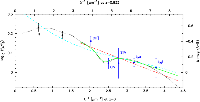
Figure 5: Different extinction laws fitted to the data from emission lines and red/infrared broad band photometry. The photometric error bars were extended to $\pm 0.05\,\mathrm{mag}$ (see text). Models with 2175 Å bump: solid (FM bump) and dotted (CCM); models without: dashed (CAB) and dot-dashed (FM nobump).

Figure 4 shows the emission line profiles after subtraction of the local linear continuum fit and rescaling with the estimated emission line flux ratio. Apart from subtle differences in absorption features, the emission line profiles of A and B are remarkably similar. The remaining differences seem to be largest in ${Si\textsc{iv}}$ but this is a result of the weakness of this line which also leads to the relatively large photometric uncertainty shown in Fig. 3.

The differences of the absorption left of Ly $\beta$ are a result of the very different relative strength of the absorption systems in A and B. Altogether the profiles are highly consistent, leaving very little doubt about the lensed nature of the two images.

The emission line ratios determined from the wide (complete line) and narrow (line core) windows are also compatible with each other. This means that the microlensing signal is the same for the broad and narrow line regions. Since the two are expected to be very different in size, the effect would be different if there is any effect at all. This means that microlensing seems to be absent already for the broad lines. Using emission lines therefore seems a reasonable way to measure extinction curves which are unaffected by microlensing, at least in HE~0512–3329.

4 Differential extinction

To analyse the differential extinction, we fitted different empirical extinction laws to the emission line data and the photometric data in $I$ and $H$, assuming that microlensing is affecting these bands only weakly as indicated from the similarity of the extrapolated continuum and the photometric data (Fig. 3 bottom). To take into account the residual microlensing effects and flux ratio changes by variability within the time-delay, we used an error of $\sigma=0.05$ mag for the photometric data points instead of the formal error or 0.02 mag. The results are not very sensitive to this exact value.

The first extinction law is the galactic curve from Cardelli et al. (1989) which has a 2175 Å feature whose strength is correlated to the far-UV behaviour (CCM). Alternatively we used the parametrisation from Fitzpatrick & Massa (1990) once with the Drude term describing the 2175 Å bump (FM bump) and once without it (FM nobump). The strength of the bump is a free parameter independent of the global shape of the extinction law, but we fixed its position and width ($x_{0}=4.6\,\mathrm{\muup m^{-1}}$, $\gamma=0.95\,\mathrm{\muup m^{-1}}$). We neglected the far-UV term $c_{4}\,F(x)$ (Fitzpatrick & Massa 1990, eq. 2) because it becomes important only at shorter wavelengths and is thus only very weakly constrained. The inclusion would actually increase the normalized $\chi^{2}$ of the fits. The strength of the 2175 Å feature does not depend on the far-UV term. Although the FM models are valid only for $\lambda^{-1}\gtrsim 3.3\,\mathrm{\muup m^{-1}}$, we included the $H$ and $I$ data in the fit using an extrapolation. The FM plots should therefore only be seen as illustrations and not as physical models. Without $H$ and $I$ these curves would rise on the left to match C iii] more closely, without changing the 2175 Å bump very much. As a second extragalactic model we used the functional form from Calzetti et al. (2000) (CAB) without a 2175 Å feature. All extinction law fits are shown in Fig. 5.

We see that all of these models fit the data relatively well; the normalized $\chi^{2}$ values are all close to unity. To follow the slightly deviating value from the C iv line more closely, however, the 2175 Å bump has to be included which also shows in improved residuals for the CCM and FM bump models. Since the C iv line lies in a region of the spectrum were the continuum is very well defined, there is no reason to trust this data point less than the others. Our result can therefore be seen as a marginal detection of the 2175 Å feature in the spectrum of HE~0512–3329. This interpretation is supported by the fact that the free fit of the absorption feature in the FM bump model favours a strength almost exactly equal to the galactic CCM model.

For the physical interpretation we only consider the galactic CCM law

$$\frac{A(\lambda)}{A(V)}=a(\lambda^{-1})+\frac{b(\lambda^{-1})}{R_{V}}$$ (1)

with $R_{V}=A(V)/E(B-V)$. The functions $a$ and $b$ are defined piecewise over a region $0.3\,\mathrm{\muup m^{-1}}\leq\lambda^{-1}\leq 10\,\mathrm{\muup m^{-1}}$ (Cardelli et al. 1989). For the differential extinction law for $\mathrm{A}-\mathrm{B}$ we obtain

$$A^{\mathrm{A}}(\lambda)-A^{\mathrm{B}}(\lambda)=p_{a}\,a(\lambda^{-1})+p_{b}\,b(\lambda^{-1})$$ (2)

with the two independent parameters

$$p_{a} = A^{\mathrm{A}}(V)-A^{\mathrm{B}}(V)$$ (3)

$$p_{b} = \frac{A^{\mathrm{A}}(V)}{R^{\mathrm{A}}_{V}}-\frac{A^{\mathrm{B}}(V)}{R^{\mathrm{B}}_{V}}\quad\mbox{.}$$ (4)

The first parameter $p_{a}$ is the differential visual extinction, the second one is the differential colour excess $p_{b}=E^{\mathrm{A}}(B-V)-E^{\mathrm{B}}(B-V)$. The difference of measured magnitudes is equal to the difference in intrinsic brightness (caused by different amplification and variability in combination with the time-delay) $p_{0}$ plus the difference in extinction. We therefore have three free parameters.

Table 1: Parameters of CCM model fits in magnitudes. $p_{0}$ is the ‘true’ brightness difference, corrected for extinction but including the different lens amplifications. $p_{a}$ is the differential extinction in $V$, $p_{b}$ is the differential colour excess. The effective $R_{V}$ is calculated as $p_{a}/p_{b}$. It is the value of $R_{V}$ if the shape of the extinction laws in A and B would be equal or if extinction is affecting only one component. The first two lines show a free fit including $1\,\sigma$ error bars, $R_{V}^{\mathrm{eff}}$ was fixed for the other lines.

$p_{0}$	$p_{a}$	$p_{b}$	$R_{V}^{\mathrm{eff}}$	$\phantom{0}\chi^{2}/\nu$
$-0.493$	$-0.074$	$+0.037$	$-2.00$	$\phantom{0}3.2/4$
$\pm 0.11\phantom{0}$	$\pm 0.11\phantom{0}$	$\pm 0.015$	(free fit)
$-0.672$	$+0.131$	$+0.059$	$+2.20$	$\phantom{0}6.1/5$
$-0.733$	$+0.206$	$+0.067$	$+3.10$	$\phantom{0}8.8/5$
$-0.870$	$+0.447$	$+0.077$	$+5.80$	$34.3/5$

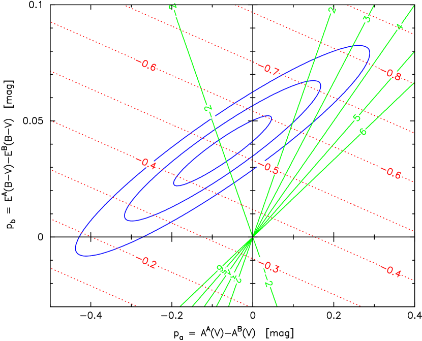
Figure 6: Residuals for fixed parameters $p_{a}$ and $p_{b}$ of the CCM model. The ellipses show differences of $\chi^{2}$ from its minimal value of $1$, $4$ and $9$ corresponding to confidence limits of $1$, $2$ and $3\,\sigma$ for one parameter. The solid lines intersecting at $(0,0)$ show the effective $R_{V}=p_{a}/p_{b}$. We see that the data are compatible with one value of $R_{V}$ only if this value is very low. The best fit has $p_{a}/p_{b}=-2.00$. The dotted parallel lines show the fitted $p_{0}$ which gives the true amplification ratio of the images.

The parameters of the best fit are shown in Table 1. We see that the visual extinction $A(V)$ has to be higher in B by 0.07 mag but the reddening $E(B-V)$ is higher in A by 0.04 mag. Recall that $A(V)$ and $E(B-V)$ are not measured directly in $V$ and $B$ but are merely used as parameters to describe and fit the UV extinction law. Figure 6 shows residuals of fits with different fixed values of $p_{a}$ and $p_{b}$. The data are only marginally compatible with only one value of $R_{V}$ (same value in both images or extinction in only one of the images) in the realistic region of $2.2<R_{V}<5.8$. The best effective $R_{V}=p_{a}/p_{b}$ is $-2.00$ which can only be explained with a combination of extinction both in A and B with different $R_{V}$. To explain the measurements with the smallest possible visual extinction, $R^{\mathrm{A}}_{V}$ must be at its lower and $R^{\mathrm{B}}_{V}$ at its upper limit. For $R^{\mathrm{A}}_{V}=2.2$ and $R^{\mathrm{B}}_{V}=5.8$ we get $A^{\mathrm{A}}(V)=0.177\,\mathrm{mag}$ and $A^{\mathrm{B}}(V)=0.251\,\mathrm{mag}$. For more similar extinction laws, the total extinction has to be higher, e.g. $A^{\mathrm{A}}(V)=0.668\,\mathrm{mag}$ and $A^{\mathrm{B}}(V)=0.742\,\mathrm{mag}$ for $R^{\mathrm{A}}_{V}=3$ and $R^{\mathrm{B}}_{V}=4$. Such values are not atypical for galactic extinction. Even with more similar $R_{V}$ the total extinction does not become unrealistically high.

The highly significant differences between continuum and emission line ratios (Fig. 3) show the importance of microlensing when studying differential extinction curves. Using photometric data points without correcting for microlensing like in Falco et al. (1999) would in the case of HE~0512–3329 lead to highly incorrect results.

An important result for lens models is the true amplification ratio which corresponds to $p_{0}=\mathrm{A}-\mathrm{B}=-0.49\pm 0.11\,\mathrm{mag}$ ($1\,\sigma$ error bar). The amplification ratio is thus $|\mu_{\mathrm{A}}/\mu_{\mathrm{B}}|=1.57\pm 0.17$. Note how different this value is from the continuum or emission line ratio in the UV (Fig. 3). The combination of extinction and microlensing changes the continuum flux ratio at the short wavelength end by almost 2 magnitudes. One should therefore be very careful when using optical flux ratios as constraints for the amplification ratio in lens modelling if no correction for microlensing and differential extinction can be applied. The result for $|\mu_{\mathrm{A}}/\mu_{\mathrm{B}}|$ depends on the emission lines only. Variations of the continuum during the time-delay (see estimate below) would not change this ratio. Variations of the emission lines are still a possible source of error here but are expected to be much smaller because of the much larger size of the emitting regions.

5 The lensing galaxy

The available observational data are quite insufficient to constrain realistic lens models to a satisfying degree. Since not even an estimate of the galaxy position is available, the best we can do at the moment is to use the simplest model, a singular isothermal sphere without external perturbations, and estimate the mass with this approach. In contrast to the time-delay, the mass depends only weakly on the exact galaxy position or asymmetries of the mass distribution.

With the source redshift $z_{\mathrm{s}}=1.58$ and a proposed lens redshift $z_{\mathrm{d}}=0.933$, this leads to an expected radial velocity dispersion of $\sigma_{v}=192\,\mathrm{km\,s^{-1}}$ and an enclosed mass within the Einstein radius of $M_{\mathrm{E}}=6.8\cdot 10^{10}\,M_{\sun}$. Using the Tully-Fisher relation for late-type galaxies at intermediate redshift (Ziegler et al. 2002), we obtain an absolute luminosity of $M_{B}=-22\,\mathrm{mag}$ using an equivalent circular velocity of $v_{c}=330\,\mathrm{km\,s^{-1}}$. This corresponds to an apparent $I$ magnitude of $21.5\,\mathrm{mag}$, about 4.5 mag weaker than each QSO component. Direct images taken with STIS in the same campaign do not show any obvious sign of the core of the lensing galaxy after applying a standard subtraction of the two QSO images. We are currently working on new methods to optimize this PSF subtraction process.

The maximal time-delay would be reached if the lens is located very close to one of the images, leading to a limiting value of 170 days. For this scenario a very high ellipticity of the mass distribution would be required. More realistic values are $\sim\,$1–2 months. A spherically symmetric lens with a true amplification ratio of 1.57 (the result of the previous section and assuming negligible variability) would lead to a time-delay of $\Delta t=38\,$days with A leading. Even a moderate ellipticity or external shear could change this number (even its sign) considerably.

6 Microlensing

With the measurement of the emission line flux ratios, we were able to obtain estimates of the differential extinction. Since the continuum is affected by extinction and microlensing, we have to remove the extinction effect to study the microlensing signal alone. Figure 7 shows the continuum flux ratio corrected for differential extinction as determined from the emission lines. Given the high uncertainties in estimating the extinction law, we do not show the estimated global microlensing function but only the values for the wavelengths of the emission lines which have been measured directly and which are thus not model dependent.

These data points should be flat zero in the absence of microlensing. We see that in reality either B is amplified and/or A is de-amplified with a strength increasing for smaller wavelengths.

An additional complication is the possibility of variability. Because of the time-delay, the two components are observed in two different epochs in the source plane. If the source brightness or spectrum changes significantly over this time-delay, the measured ratio would not reflect the true ratio anymore. Assuming that this effect is negligible in our observations of HE~0512–3329, we can use the magnitude of the differential microlensing to estimate an upper limit for the source size in terms of the Einstein radius using the recipe of Refsdal & Stabell (1991). If the observed differential microlensing signal of $\delta m=0.5\,\mathrm{mag}$ is typical for the microlensing variance, a conservatively estimated upper limit of 4 Einstein radii can be derived. The Einstein radius in our case is $\theta_{\mathrm{e}}=1.2\,\muup\mathrm{arcsec}\cdot\sqrt{M/M_{\sun}}$ for microlenses of mass $M$, corresponding to $0.01\,\mathrm{pc}$ ($2200\,$AU) in the source plane for $M=M_{\sun}$.

We also tried to fit the parameters of more specific physical scenarios like isolated caustic crossings of a standard accretion disk model to the data, only to learn that (although this should be a powerful method in principle) the available data are not sufficient to obtain any conclusive results.

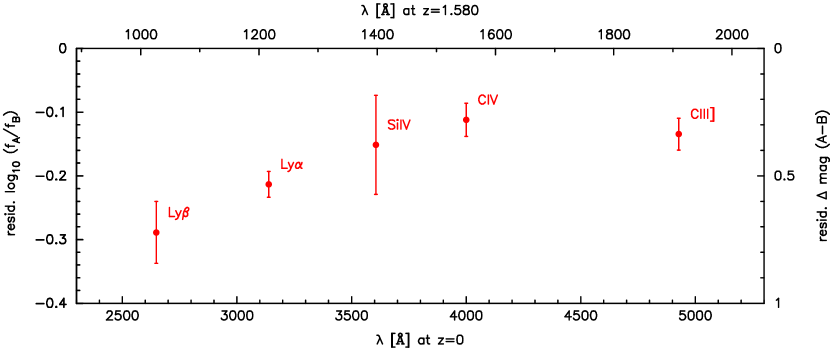
Figure 7: Differential microlensing amplification ($A/B$) as a function of wavelength (error bars). The continuum (affected by microlensing and extinction) was corrected for extinction using the emission line fluxes which are expected to be unaffected by microlensing.

7 Summary

We presented the first separate spectra of both components of the doubly lensed QSO HE~0512–3329. The similarity of the optical and near UV spectra strongly suggest the lens nature of this object.

The known optical colour differences of the images, which (together with the metal absorption lines) were the main motivation to start this project, extend to the near UV and become even stronger in this range. While A is brighter than B by about 0.5 mag in $R$ and $I$ band, this relation is more than inverted in the continuum near $2000\,\mbox{\AA}$ where B is brighter by about 1.3 mag.

We used the continuum subtracted emission line flux ratios to study the differential extinction in both images. The line emitting regions of the QSO are confirmed to be so large that any residual microlensing effects on their fluxes is insignificant so that the extinction can be studied unambiguously. We fitted several empirical extinction laws from the literature and found that curves with a significant 2175 Å bump (CCM: Cardelli et al. 1989; FM bump: Fitzpatrick & Massa 1990) reproduce the data better than typical extragalactic curves without this feature (FM nobump: Fitzpatrick & Massa 1990; CAB: Calzetti et al. 2000). Although the differences are not highly significant, this provides at least evidence that the 2175 Å feature can also be present in high redshift galaxies (compare Motta et al. 2002).

From the difference between the emission line and continuum ratios we learned that microlensing contributes significantly to the variations of flux ratio with wavelength. On the short wavelength end, the microlensing signal is actually much stronger than the differential reddening. While the emission lines have almost the same flux in A and B there, the continuum is brighter in B by up to 1.3 mag (see Fig. 3 bottom). For our study it was therefore absolutely essential to use the emission line fluxes for the extinction analysis. Analysing the continuum or broad band photometry like in Falco et al. (1999) without correcting for microlensing would have led to highly incorrect results in the case of HE~0512–3329.

The analysis of galactic extinction law fits showed that the data are only marginally consistent with the same extinction law in A and B with only different strength. The best fit has a higher total visual extinction $A(V)$ in B but a higher reddening $E(B-V)$ in A.

Using the image separation, we were able to estimate the mass within the Einstein radius to be $M_{\mathrm{E}}=6.8\cdot 10^{10}M_{\sun}$. The expected radial velocity dispersion of an isothermal model is $\sigma_{v}=192\,\mathrm{km\,s^{-1}}$, equivalent to a circular velocity of $v_{c}=330\,\mathrm{km\,s^{-1}}$. The time-delay is expected to be of the order 1–2 months.

In the last part we used the differential extinction measurement from the emission lines to correct the continuum flux ratio at five wavelengths for this effect. The remaining ratio is a direct measurement of the microlensing signal alone. This is the first time that such a study is carried out to separate the two effects and discuss them individually.

The microlensing data are not sufficient to determine the parameters of physically motivated source models accurately but could be used to estimate an upper limit for the effective source size using the assumption that variability over a scale of the time-delay does not change the observed flux ratio significantly. To test this assumption and to determine the time-delay, photometric monitoring of this system should be performed in the future. The information gained by our work (spectral microlensing measurements at one epoch) is complementary to the more common light-curve analysis technique (photometric measurements at many epochs, see e.g. Shalyapin et al. 2002 for recent results). A combination of both methods by using spectrophotometric monitoring data has the potential to lead to more valuable constraints than both methods alone by breaking degeneracies inherent in the individual approaches. It will then be possible to determine brightness profiles in all of the measured wavelengths which can be combined to a relatively model-independent measurement of the source’s temperature profile, allowing to test different physical QSO models.