On the size difference between red and blue globular clusters

Abstract

Several recent studies have reported a mean size difference of about 20% between the metal-rich and metal-poor subpopulations of globular clusters (GCs) in a variety of galaxies. In this paper we investigate the possibility that the size difference might be a projection effect, resulting from a correlation between cluster size and galactocentric distance, combined with different radial distributions of the GC subpopulations. We find that projection effects may indeed account for a size difference similar to the observed one, provided that there is a steep relation between GC size and galactocentric distance in the central parts of the GC system and that the density of GCs flattens off near the center in a manner similar to a King profile. For more centrally peaked distributions, such as a de Vaucouleurs $R^{1/4}$ law, or for shallower size-radius relations, projection effects are unable to produce the observed differences in the size distributions.

1 Introduction

Since the work of Kinman (1959) and Zinn (1985), it has been known that globular clusters in the Milky Way can be divided into (at least) two sub-populations with distinct kinematical and chemical properties. Undoubtedly one of the most important developments in research on globular clusters (GCs) within the last decade is the discovery that similar substructure is seen in the color (and hence, presumably, metallicity) distributions of GC systems in many early-type galaxies (Zepf & Ashman, 1993; Gebhardt & Kissler-Patig, 1999; Kundu & Whitmore, 2001; Larsen et al., 2001). There is increasing evidence that GC sub-populations in early-type galaxies share many properties with those in spirals (Forbes, Brodie, & Larsen, 2001), and that the GCs in different galaxy types may be closely related. Characterizing and understanding the properties (spatial and metallicity distributions, kinematics etc.) of GC sub-populations is currently a subject of much investigation and holds the promise of revealing important information about events in the evolution of their host galaxies.

One piece of the puzzle is to establish just how similar are GCs in different galaxies. The Hubble Space Telescope can resolve the spatial profiles of globular clusters well beyond the Local Group, although careful modeling of the undersampled point spread function (PSF) of the WFPC2 camera is necessary in order to derive reliable size information for typical extragalactic GCs. Kundu & Whitmore (1998) were among the first to measure the sizes of extragalactic GCs and found that GCs in the lenticular galaxy NGC 3115 had half-light radii of about 2 pc, similar to or perhaps slightly smaller than those in the Milky Way. When measuring sizes for the blue (metal-poor) and red (metal-rich) GC subpopulations separately, Kundu & Whitmore (1998) noted a size difference of about 20% with the red GCs being systematically smaller. A similar size difference was found between red and blue GCs in NGC 4486 (Kundu et al., 1999). Subsequently, size differences between GC subpopulations have been found in many other galaxies including NGC 4472 (Puzia et al., 1999), NGC 4594 (the “Sombrero”; Larsen, Forbes & Brodie, 2001), M31 (Barmby, Holland, & Huchra, 2002) and other early-type galaxies (Larsen et al., 2001). However, it should also be noted that Harris et al. (2002) found no size-color relation for a sample of 27 GCs in NGC 5128.

Although the results on NGC 5128 suggest that the size difference may not be universal, there seems to be compelling evidence that it is at least a wide-spread phenomenon, observed in spirals as well as in early-type galaxies. Understanding the origin of this size difference is a high priority, since any intrinsic correlation between the sizes and metallicities of star clusters might hold clues to their formation mechanisms. However, before one attempts to explain the size difference in terms of e.g. the properties of the proto-cluster clouds, variations in external pressure etc., other more straight-forward explanations need to be ruled out.

One possibility is that the observed size difference is a projection effect, resulting from a correlation between GC size ($r$) and Galactocentric distance ($R$) combined with different radial distributions of the GC subpopulations (throughout this paper, we will adopt the following convention: a small $r$ refers to the size (radius) of an individual globular cluster, while a capital $R$ refers to the distance of that cluster from the galaxy center. We will use subscripts ($R_{\rm proj}$, $R_{\rm 3D}$) to specify projected and 3-D quantities). van den Bergh, Morbey, & Pazder (1991) found that the size-$R$ relation in the Milky Way can be approximated by a square-root relation, $r\propto\sqrt{R}$, and they also noted that similar relations exist in M31, NGC 5128 and the LMC. However, because of the limited spatial coverage of HST, little is known about size-$R$ trends in other more distant galaxies.

Concerning the wide-field spatial distributions of extragalactic GC systems, most of the available information comes from ground-based studies which generally provide the only way to obtain complete coverage at large radii. In addition to the Milky Way and M31, galaxies where the radial distributions of GC sub-populations have been studied include NGC 1380 (Kissler-Patig et al., 1997), NGC 1399 (Dirsch et al., 2003), NGC 4472 (Lee, Kim, & Geisler, 1998) and NGC 4486 (Côté et al., 2001). In all of these cases, the red GC sub-population is more centrally concentrated than the blue one. Therefore, red GCs observed at a given projected radius will on average be physically closer to the galaxy center than the blue ones. Clearly, there is reason to suspect that projection effects might account for at least some of the differences in the mean sizes of GC samples. Our goal in this paper is to investigate and quantify this idea in more detail.

2 Observations: sizes of GC subpopulations

While size information is now available for many extragalactic GC systems, the spatial coverage is in most cases limited to a single WFPC2 pointing, usually centered on the galaxy. Therefore, information about variations with galactocentric distance is limited. Even with several pointings, the surface density of GCs drops off rapidly at large radii, and in all but the richest systems it is difficult to obtain reliable statistics based on the small number of clusters contained within an off-center WFPC2 field. In practice, then, the number of suitable datasets that can serve as a basis for our analysis is limited. We have selected three well-studied galaxies with multiple HST/WFPC2 pointings and rich GC systems (NGC 4472, NGC 4486 and NGC 4594). The WFPC2 data are the same as those used in Larsen et al. (2001) and we refer to that paper for details about the data reduction. Briefly, the globular cluster sizes were measured by convolving a series of analytic models with the WFPC2 PSF, adjusting the FWHM of the model until the best match to the observed profile was obtained. For this purpose, we used the ISHAPE code described in Larsen (1999). The main systematic errors involved in this process are related to che choice of model PSF and are difficult to quantify, but comparison of size measurements on different frames have indicated that this method yields FWHM values consistent to about 0.1 WF pixel for individual clusters (Larsen, Forbes & Brodie, 2001; Larsen et al., 2001). In addition, we include data for the Milky Way from Harris (1996) and M31 (size information kindly provided by P. Barmby).

As an illustration of the typical size differences between GC sub-populations, Fig. 1 shows the size distributions for GCs in each of the WFPC2 pointings for the three early-type galaxies. Here we are not concerned with the absolute values of the GC sizes so for the HST data we simply use the FWHM of the cluster profiles, measured in pixels and corrected for the WFPC2 PSF. To avoid any systematic differences due to the different pixel scales of the PC and WF chips, we only use sizes measured on the WF chips. We divide between “red” and “blue” clusters at $\mbox{$V\!-\!I$}=1.05$, corresponding roughly to a metallicity of $\mbox{[Fe/H]}\sim-1$. Table 1 lists the mean sizes of red and blue globular clusters in each of the WFPC2 fields, along with the probability $P$ (from a Kolmogorov-Smirnoff test) that the size distributions are drawn from the same parent distribution. For all of the central WFPC2 pointings, Table 1 and Fig. 1 confirm a significant difference between the size distributions of blue and red GCs ($P<0.03$), amounting to a difference of 15–30% in the mean sizes. However, at larger radii the situation is less clear: While the red GCs are smaller than the blue GCs in all of the NGC 4486 pointings except NGC 4486-E, the difference is only significant in the three innermost ones. In NGC 4472, the two outer pointings (B and C) cover roughly the same radial range, but a size difference is seen in only one of them and is only significant at the $\sim$89% confidence level. In NGC 4594, only the central pointing has enough clusters to obtain useful information about size distributions. In this central pointing there is a $\sim 15$% difference between the mean sizes of red and blue GCs and the distributions are different at the 97% confidence level.

The size distributions for Milky Way and M31 GCs are shown in Fig. 2. In the Milky Way we have adopted a division at $\mbox{[Fe/H]}=-1.0$, while the classification of clusters in M31 as metal-poor or metal-rich was based on a variety of photometric and spectroscopic criteria (Barmby et al., 2000). As previously noted (Larsen et al., 2001; Barmby, Holland, & Huchra, 2002), metal-rich and metal-poor GCs in the Milky Way and M31 display a size difference reminiscent of that observed in the early-type galaxies, but at least in the Milky Way it is likely that the difference is at least partly due to the different radial distributions of the two GC subpopulations. In Larsen et al. (2001) we tried to reduce this problem by comparing clusters in smaller radial bins, but the modest number of GCs in the Milky Way limits the extent to which such sub-division is feasible. In Sec. 3.2 below we return to this issue.

3 Modeling projection effects

3.1 GC size versus luminosity

Before we proceed, we briefly discuss one other effect which could potentially affect the comparison of mean sizes for GC subpopulations. Because the mass-to-light ratio of a single-aged stellar population (such as a star cluster) is a function of metallicity, the mass limit of a magnitude-limited sample of GCs is, in principle, also metallicity-dependent. Thus, a size-mass relation could introduce spurious size differences between magnitude-limited samples of different metallicities. Furthermore, age differences between GC sub-populations could also lead to different mass-to-light ratios. However, in the Milky Way there is a striking absence of any size-luminosity relation for GCs (van den Bergh, Morbey, & Pazder, 1991), and the same seems to be the case in early-type galaxies (Kundu & Whitmore, 2001) and even for young clusters in mergers (Zepf et al., 1999). This suggests that the magnitude (or mass) limit of the sample is largely irrelevant when comparing cluster sizes.

In Fig. 3 we plot the size measurements for globular clusters in NGC 4472, NGC 4486 and NGC 4594 as a function of their magnitude. The lines are least squares linear fits to the data, and they all have very small slopes that differ from 0 by less than $1\sigma$. Again, this suggests that the size difference cannot be explained as a result of different M/L ratios of the GC sub-populations. We note in passing that this lack of a size-luminosity relation is a very interesting and puzzling result in its own right, with the obvious implication that the mean densities of stellar clusters are directly proportional to their masses.

3.2 Revisiting the Milky Way

In order to calculate the projected size distributions of GC sub-populations, two basic ingredients are needed: 1) a relation between GC size and galactocentric distance, assumed to be the same for both (or all) GC subpopulations, and 2) density profiles, assumed to be different for each population. The size-$R$ relation is not easily constrained for extragalactic GC systems, partly because the GC sizes are close to the resolution limit of WFPC2 and small differences in telescope tracking, focusing etc. could introduce spurious effects when comparing measurements from different pointings. A more fundamental problem is that only the projected size-$R$ relations can be directly observed, while we need the run of GC size versus physical (3-D) galactocentric distance. For the following discussion we will therefore start out by assuming a relation of the form

$$r\,=\,a\sqrt{R_{\rm 3D}}\,+\,b,$$ (1)

i.e. similar to that observed in the Milky Way, but note that we have allowed for addition of a constant term to the simple square-root law suggested by van den Bergh, Morbey, & Pazder (1991). We emphasize that we do not intend to imply any physical significance of this particular relation but simply use it as a convenient fitting function. Note, also, that any intrinsic scatter in the relation (which might depend on $R_{\rm 3D}$ in non-trivial ways) is ignored.

Fig. 4 shows $r_{\rm eff}$ versus $R_{\rm 3D}$ for Milky Way GCs. The upper panel shows a least-squares fit of Eq. (1) to all clusters with size information. The best fit is

$$r_{\rm eff}=(0.87\pm 0.16\,{\rm pc})\sqrt{R_{\rm 3D}/3{\rm kpc}}\,+\,(1.79\pm 0.26\,{\rm pc}),$$ (2)

where $r_{\rm eff}$ is the effective (half-light) radius and we have normalized the relation to a scale radius of 3 kpc (roughly the median galactocentric distance of the metal-rich GCs). Of course, choosing a different scale radius is equivalent to changing the coefficient $a$. The two lower panels show the metal-poor (“blue”) and metal-rich GCs separately. Especially for the metal-rich GCs, the slope of the size-$R$ relation is very poorly constrained, but to check whether any significant size differences exist between the two GC populations we adopt the same slope as for the combined sample and just fit the constant term. For the metal-poor and metal-rich GCs this term is $b=1.76\pm 0.13$ pc and $b=1.86\pm 0.23$ pc, respectively. Formally, the constant term is now slightly larger for the metal-rich clusters, contrary to the trend seen in the projected size distributions, but the difference is not statistically significant. In practice, then, there is no evidence for a significant size difference between the two Milky Way GC populations when the radial dependence is averaged out. We therefore conclude that the size difference in Fig. 2, at least for the Milky Way, can be fully explained as a result of the different radial distributions of the two GC subpopulations.

3.3 Extragalactic GC systems

While ground-based data offer superior coverage at large radii compared to most HST datasets, completeness issues are more severe near the center. However, in order to model the GC size distributions it is important to know the behavior of the spatial distributions of GCs near the center, as well as at larger distances. Of the HST datasets used here, NGC 4486 has the best radial coverage, extending out to 9$\arcmin$. In Fig. 5 we show the GC surface densities as a function of projected distance from the galaxy center (in arcmin) for the two GC subpopulations. It is evident that the red GCs are much more centrally concentrated. We have adopted a magnitude limit of $V=24$, which is 1.5 mag brighter than the 50% completeness limit even in the central pointing (Larsen et al., 2001), so we do not expect completeness effects to be significant except perhaps in the central 20$\arcsec$–30$\arcsec$. Also superimposed on the plots are de Vaucouleurs $R^{1/4}$ laws and King (1966) profiles. For the King profiles we have arbitrarily fixed the concentration parameter at $R_{\rm tidal}/R_{\rm core}=20$. The two best-fitting de Vaucouleurs profiles have effective radii of $2\arcmin$ (red clusters) and $24\arcmin$ (blue clusters), although these numbers are rather sensitive to the background correction. The two King profiles have effective radii of $2\farcm 05$ and $4\farcm 56$, a much smaller difference than for the de Vaucouleurs profiles, but note that our radial coverage only extends out to about 1/3 of the half-light radius of the de Vaucouleurs fit to the blue GC distribution.

In the outer, poorly constrained regions, the King profiles decline more rapidly than the $R^{1/4}$ law, resulting in the very different half-light radii for the two types of profiles. In fact, a fundamental difference between the King and de Vaucouleurs profiles is that the former has a well-defined tidal radius, while the latter does not. However, our primary objective here is not to obtain a correct fit at very large galactocentric distances (which contribute with only a few clusters in projection), but merely to find appropriate “fitting functions” that allow us to model the spatial distributions of GCs and deproject the observed surface densities to obtain estimates of 3-D space densities. Fig. 5 suggests that the King profiles provide a fit that is at least as good as an $R^{1/4}$ law in the inner regions, and probably better.

One remaining issue is to convert the observed surface density profiles to space densities, $\rho(R_{\rm 3D})$. For the de Vaucouleurs profiles we use the series expansion tabulated by Bendinelli, Ciotto & Parmeggiani (1993). For the King profiles, the space density is automatically obtained during the process of computing the King model.

3.4 Projected mean properties of GC sub-populations

Near the center, the King profiles flatten out whereas the de Vaucouleurs profiles diverge. This difference in behavior has important implications for the projected properties of GC systems distributed according to either of the two profiles. To illustrate this point, consider the mean 3-D distance $\langle R_{\rm 3D}\rangle$ of GCs observed at a given projected distance $R_{\rm proj}$. These are related as

$$\langle R_{3D}\rangle_{R_{\rm proj}}\,=\,\frac{\int_{R_{\rm proj}}^{R_{\rm max}}R_{\rm 3D}\,n(R_{\rm 3D})dR_{\rm 3D}}{\int_{R_{\rm proj}}^{R_{\rm max}}n(R_{\rm 3D})dR_{\rm 3D}}$$ (3)

where

$$n(R_{3D})\equiv\frac{R_{3D}\rho(R_{3D})}{\sqrt{R_{3D}^{2}-R_{\rm proj}^{2}}}$$ (4)

The upper integration limit, $R_{\rm max}$, should in principle be set to the outer radius of the GC system. This is a poorly constrained, but relatively uncritical number as the density in the outer parts is very low. We will generally adopt $R_{\rm max}=20\,\mbox{$R_{\rm eff}$}_{R}$, where $\mbox{$R_{\rm eff}$}_{R}$ is the effective radius of the red GC subpopulation. This is well beyond the limit where reliable data exists for most GC systems.

Fig. 6 shows $\langle R_{3D}\rangle$ as a function of $R_{\rm proj}/\mbox{$R_{\rm eff}$}_{R}$ for de Vaucouleurs and King profiles corresponding to the fits in Fig. 5. The straight dotted line in each figure is simply a 1:1 relation, plotted for reference. Fig. 6 shows that, at any $R_{\rm proj}$, the “blue” GCs are indeed located at significantly larger mean distances from the galaxy center than the red ones. For the de Vaucouleurs profile, most of the clusters observed near the center are also located at small physical distances from the center. For the King profiles, which flatten out near the center, the mean 3D distance from the center at $R_{\rm proj}=0$ is substantially larger than for the de Vaucouleurs profiles.

In a similar fashion to Eq. (3), the mean cluster size $\langle r\rangle$ at $R_{\rm proj}$ is

$$\langle r\rangle_{R_{\rm proj}}\,=\,\frac{\int_{R_{\rm proj}}^{R_{\rm max}}r(R_{\rm 3D})n(R_{\rm 3D})dR_{\rm 3D}}{\int_{R_{\rm proj}}^{R_{\rm max}}n(R_{\rm 3D})dR_{\rm 3D}}$$ (5)

3.5 Application to the M31 GC system

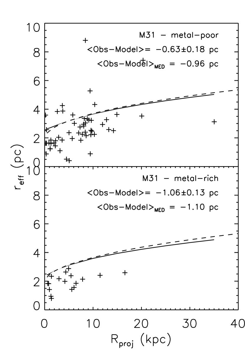
Figure 7: Size vs. projected galactocentric distance for GCs in M31. In each panel, the solid and dashed lines show the mean sizes obtained by projecting the Milky Way size-$R_{\rm proj}$ relation for King and de Vaucouleurs GC density profiles, respectively.

In Fig. 7 we apply Eq. (5) to the M31 GC system, adopting the same size-$R$ relation as in the Milky Way. The top and bottom panels show GC size vs. projected galactocentric distance for metal-poor and metal-rich GCs, respectively. As noted by other authors, there is a clear trend of GC size increasing with $R$ for the M31 GCs (Crampton et al., 1985; Barmby, Holland, & Huchra, 2002). Note, however, that the samples of M31 GCs are likely to suffer from severe selection effects, making the spatial distributions uncertain (Barmby et al., 2000).

In each panel of Fig. 7, the solid and dashed lines represent the size-$R$ relations obtained by projecting the Milky Way relation (Eq. 2) using King and de Vaucouleurs GC density profiles with effective radii of 17$\arcmin$ and 30$\arcmin$. These effective radii are based on the data in Barmby et al. (2000) and are rather similar to those for the Milky Way GC system. The first impression is that the projected Milky Way relation appears to overestimate the GC sizes in M31, but this may be partly due to the fact that the Milky Way contains a number of GCs with large sizes which shift the mean relation upwards. Such clusters are not detected in M31, but could well have evaded detection especially near the center of the galaxy where the bright background from the bulge and disk makes it difficult to see low-surface brightness, extended objects.

As indicated in the Figure, the mean differences between observed and model sizes are $-0.63\pm 0.18$ pc and $-1.06\pm 0.13$ pc for the metal-poor and metal-rich GCs, respectively. Thus, in addition to the systematic offset between modeled and observed relations, there is a 0.4 pc difference between metal-rich and metal-poor clusters which is formally unaccounted for by simple projection of the Milky Way size-$R$ relation. However, there are several outlying datapoints, especially in the upper panel. The median is less sensitive to such outliers, and if we use the median instead of mean as an indicator of the difference between model and observations (labeled $\langle{\rm Obs}-{\rm Model}\rangle_{\rm MED}$ in Fig. 7) then the difference is reduced to 0.14 pc. In summary, it seems quite likely that the size difference between the GC sub-populations in M31 may again be explained largely as a result of differences in the radial distributions, as in the Milky Way, although it would desirable to confirm this with size measurements for a larger sample of clusters.

3.6 Projected GC size vs. radius trends in the HST datasets

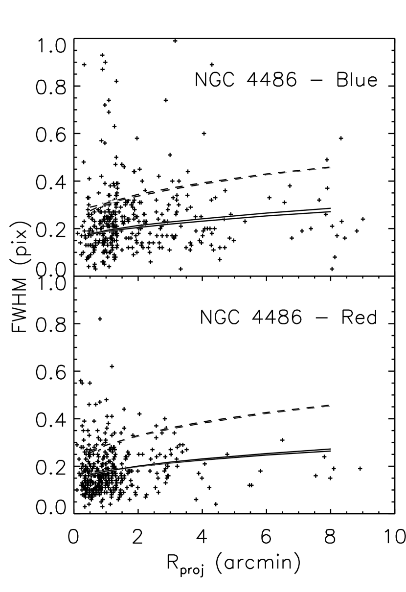
Figure 8: Size vs. projected galactocentric distance for GCs in NGC 4486. The dashed curves show the mean sizes obtained by projecting the Milky Way size-$R_{\rm proj}$ relation for King and de Vaucouleurs GC density profiles. The solid curves represent a relation with half the slope of the Milky Way relation and a zero-point shifted downwards to roughly match the NGC 4486 data.

NGC 4472 and NGC 4486 are both located in the Virgo cluster, for which we will assume a distance of 15 Mpc. NGC 4594 is somewhat closer, at a distance of about 9 Mpc (Ford et al., 1996). At 15 Mpc, 1 WF pixel corresponds to 7.3 pc. With a conversion factor of 1.48 between the FWHM and half-light radii of the King models used to fit the cluster profiles, the Milky Way relation (Eq. 2) then translates to ${\rm FWHM}\,\approx\,(0.08\,{\rm pixels})\sqrt{R_{\rm 3D}/0\farcm 7}\,+\,0.17$ pixels (where the scale radius of 3 kpc corresponds to $0\farcm 7$ at the assumed distance). It is, however, not obvious just how to apply the Milky Way size-$R_{\rm 3D}$ relation to other galaxies. In Fig. 8 we display the size measurements for red and blue GCs in NGC 4486 as a function of $R_{\rm proj}$. The radial range, $10\arcmin$ or 44 kpc, is roughly similar to those for the Milky Way and M31 plots in Fig. 4 and Fig. 7. In each panel, the mean size vs. $R_{\rm proj}$ relation obtained by projecting the Milky Way relation is shown with dashed lines, using Eq. (5) and the King and de Vaucouleurs profiles from Fig. 5. At the scale and radial range of this figure, the two model GC surface density profiles give very similar mean size vs. $R_{\rm proj}$ relations.

While the sizes are measured on several WFPC2 pointings and systematic differences might be present from one pointing to another, it is undeniable that the Milky Way relation applied directly provides a rather poor fit to the NGC 4486 data. Part of the mismatch might be due to systematic errors in the PSF modeling, which could shift all datapoints up or down, but application of the Milky Way relation also gives a too steep slope. There is, of course, no particular reason why the size-$R$ relations should be the same in the Milky Way and in NGC 4486. The solid lines in Fig. 8 show the size-$R_{\rm proj}$ relation obtained by projecting a size-$R_{\rm 3D}$ relation with half the slope of that in the Milky Way and shifted downwards by 0.05 pixel. This provides a much better match to the observations, although the match remains less than satisfactory in the outer regions. Note that, instead of explicitly applying a shallower slope to the size-$R_{\rm 3D}$ relation, we could have normalized $R_{\rm 3D}$ to a 4 times larger scale radius. Although the physical basis for the size-$R$ relation is poorly understood, it is interesting to note that half-light radius of the red GC population in NGC 4486, $2\arcmin$ or 9 kpc, is also roughly 3–4 times larger than that of the metal-rich Milky Way GCs.

The other HST datasets do not provide additional constraints on any size-$R$ relation for GCs, as illustrated in Fig. 9 where we compare GC size vs. $R_{\rm proj}$ for NGC 4472, NGC 4486 and NGC 4594. For the other two galaxies the radial range is more limited and in NGC 4594 the number of clusters in the outer parts is very small (note that the NGC 4594 data cover a smaller radial range in kpc, due to the smaller distance of this galaxy). However, the behavior of GC size vs. $R_{\rm proj}$ in these galaxies does not appear to be significantly different from that in NGC 4486. Though the fit to the NGC 4486 data may be further improved by additional iterations on the input size-$R_{\rm 3D}$ relation, we will adopt the half-slope, zero-point shifted relation in Fig. 8 for the following discussion, given as

$$\mbox{FWHM}\,=\,(0.12\,{\rm pixels})\,+\,(0.04\,{\rm pixels})\sqrt{R_{\rm 3D}/0\farcm 7}$$ (6)

Fig. 10 shows the ratio of the mean sizes of “blue” and “red” GCs as a function of projected galactocentric distance, calculated according to Eq. (6) and using the GC surface density profile fits in Fig. 5. The solid and dashed lines are for the de Vaucouleurs and King profiles, respectively. In addition, the dotted line shows the ratio for King profiles for which the effective radii of the blue and red GC surface density distributions differ by a factor of 4 (instead of $\sim 2.3$). The projected radius $R_{\rm proj}$ is plotted in units of the effective radius of the red GC population. Near the center, a difference of about 12% in the mean sizes is indeed produced for the King profiles, while the size difference remains below 10% for the de Vaucouleurs profiles. At larger radii the size difference decreases regardless of the choice of model. While the details of Fig. 10 clearly depend on many poorly constrained parameters, it provides another hint that projection effects might account, at least partially, for the differences between the projected size distributions of metal-rich and metal-poor GCs.

3.7 Modeling the size distributions

A lot of useful information is lost by simply averaging over the size distributions and comparing mean sizes. Even if the average trends are reproduced, the detailed behavior of the observed distributions might not be properly accounted for. Instead, it is more illustrative to directly compare the predicted size distributions with the observations.

At a given projected distance $R_{\rm proj}$, the number of clusters $N(R_{\rm 3D})dR_{\rm 3D}$ in a small radial range $dR_{\rm 3D}$ around $R_{\rm 3D}$ is proportional to the right-hand side of Eq. (4). It follows that the size distribution, expressed as the number of clusters $N(r)dr$ in a small size bin $dr$ centered on $r$ can be expressed as

$$N(r)dr\,=\,\frac{\rho\,R_{\rm 3D}}{\sqrt{R_{\rm 3D}^{2}-R_{\rm proj}^{2}}}\frac{dR_{\rm 3D}}{dr}\,dr$$ (7)

where it is assumed that $r$ is a monotonic function of $R_{\rm 3D}$ so that the inverse function $R_{\rm 3D}(r)$ exists. Note also that the space density of clusters, $\rho$, must be evaluated at the appropriate radius, $R_{\rm 3D}(r)$.

The distribution functions for $R_{\rm 3D}$ (Eq. 4) at various projected radii are shown in Fig. 11 for King profiles (a) and de Vaucouleurs laws (b). Each panel shows the $R_{\rm 3D}$ distribution functions for projected radii of $R_{\rm proj}=0.0$, 0.5 and 1.0. The solid lines are for models with effective radii of 1.0 (both panels). Following the fits to the NGC 4486 GC system (Fig 5), the dashed lines show King models with $\mbox{$R_{\rm eff}$}=2.3$ (a) and de Vaucouleurs models with $\mbox{$R_{\rm eff}$}=10$ (b). For both models the $R_{\rm 3D}$ distributions are strongly peaked near $R_{\rm proj}$ and quite similar for models with different effective radii, except for the King models near the center. Hence, the most significant differences in the size distributions of blue and red GCs are expected near the center, and should be much more noticeable for King density profiles.

In Fig. 12 we show the projected size distributions at the same $R_{\rm proj}$ as in Fig. 11, using the size-$R_{\rm 3D}$ relation for NGC 4486 from Fig. 8 (Eq. 6). As suspected, the King and de Vaucouleurs laws produce very different size distributions near the center. Even though the de Vaucouleurs law does produce a difference in the mean sizes (though smaller than for the King profiles), this is mainly due to a more extended “tail” in the size distribution of the blue clusters. For the King profiles, on the other hand, the simulated size distributions show two clearly separated peaks near the center, more akin to the observed distributions. Changing the constant term ($b$) in Eq. (1) simply shifts both distributions horizontally, while changing the scale factor ($a$) changes the width of the two distributions and their separation.

In Fig. 13 we compare the observed size distributions in NGC 4486 with our simple model. Panel (a) shows the size distributions obtained by projecting the square-root size-$R_{\rm 3D}$ law (Eq. 6) at 15–30 discrete $R_{\rm proj}$ (hence the jagged appearance of some of the curves), spanning the radial range covered by each WFPC2 field. The individual contributions were weighted by the azimuthal coverage of the WFPC2 field at the corresponding $R_{\rm proj}$. We have not attempted to normalize the model distributions to the observed numbers of clusters in each bin, although the relative numbers of red and blue clusters do change according to the assumed (King) surface density profiles. The observed and modeled number ratios N(red)/N(blue) are listed for each for each WFPC2 pointing in Table 2 and agree within the uncertainties, except perhaps for the outermost pointing where deviations from the King profile may begin to become apparent.

While the simulated size distributions in Fig. 13 (a) do show a significant difference between red and blue GCs, the offset between the two distributions is clearly not as pronounced as for the actual observed distributions. Thus, at least for the simple square-root law, it is difficult to fully explain the size difference as a projection effect. In order to obtain a wider separation between the peaks of the two GC size distributions, we need a steeper relation between GC size and galactocentric distance in the central parts of the GC system. However, adopting a steeper slope for the square-root law would be incompatible with the relatively flat size-$R_{\rm 3D}$ trend observed at larger radii (Fig. 9). We therefore need a curve which is steeper at small radii compared to the square-root law, but flattens out at large radii. One possibility is to use a relation consisting of two linear segments:

$$\mbox{FWHM}\,=\left\{\begin{array}[]{lr}a_{1}R_{\rm 3D}+b_{1}&\mbox{for }R_{\rm 3D}<R_{1}\\ a_{2}R_{\rm 3D}+b_{2}&\mbox{for }R_{\rm 3D}>R_{2}\end{array}\right.$$ (8)

with $R_{2}>R_{1}$ and using a cubic spline to interpolate between the two linear segments in the interval $R_{1}<R_{\rm 3D}<R_{2}$. Just piecing a relation together directly from two linear segments with an abrupt change in slope at a certain radius will not work, because the term $dR_{\rm 3D}/dr$ in Eq. (7) will then be discontinuous, leading to a “jump” in the size distribution. However, by choosing an adequate separation between $R_{1}$ and $R_{2}$ the change in slope will be gentle enough to avoid spurious effects in the resulting size distribution. After some experimentation, we found that a reasonable match to the observed size distributions was obtained for $a_{1}=0.07$ pixels arcmin^-1, $b_{1}=0.05$ pixels, $R_{1}=1\farcm 5$, $a_{2}=0.005$ pixels arcmin^-1, $b_{2}=0.21$ pixels and $R_{2}=4\farcm 5$. The curve corresponding to these coefficients is compared with the square-root law in Fig. 14 and in panel (b) of Fig. 13 we show the corresponding size distributions. By construction, the match to the observed size distributions is now much better in the inner pointing (uppermost panel), though the model now appears to actually overpredict the size difference in the range $0\farcm 10<R<3\farcm 10$. The “tail” extending up to sizes $>0.5$ pixels in the observed distributions is not reproduced in any of the model distributions, but may well be due to intrinsic and/or measurement scatter in the GC size distributions, which is not taken into account in our simple model. Probably for the same reason, the simulated distributions in the outer pointings are much more peaked than the observed ones. Regardless, Fig. 13 (b) shows that projection effects can indeed produce size differences that are quite similar to the observed ones.

Finally, we caution against over-interpreting Fig. 13. It should be emphasized that the measured GC sizes are only a fraction of a WFPC pixel and any differences in mean size from one panel to another are probably only marginally significant. For example, Table 1 indicates a decrease in the mean cluster size from field NGC 4486-C to NGC 4486-D of about 0.06 pixels, which is almost certainly an artifact. The random rms error on the size measurements is about 0.1 pixel (Larsen et al., 2001) and may account for a significant fraction of the widths of the observed size distributions, although the Milky Way data suggests that some intrinsic scatter is also present.

4 Summary and concluding remarks

We have re-examined the size distributions of globular cluster sub-populations in three early-type galaxies with HST/WFPC2 imaging, as well as those in the Milky Way and M31. As in previous studies, we find that the blue clusters are, on average, larger than the red ones. The difference is, however, most pronounced in the central parts of the galaxies, and its statistical significance decreases strongly at larger radii.

In order to test whether the size difference might be a projection effect, resulting from a correlation between cluster size and galactocentric distance combined with different radial distributions of the GC subpopulations, we first fitted a square-root law to size vs. galactocentric distance ($R_{\rm 3D}$) for metal-rich and metal-poor GCs in the Milky Way. Within the uncertainties, the two GC sub-populations in the Milky Way appear to follow the same size-$R_{\rm 3D}$ relation. For extragalactic GC systems, only projected size distributions can be observed. In general, the size distributions observed at a given projected galactocentric distance will depend on the relation between GC size and 3-D galactocentric distance, as well as the 3-D density profiles of the two GC populations. These relations are poorly constrained by current data, but we have explored a limited number of analytical approximations that seem to be adequate for the NGC 4486 GC system (for which the best data are available). Specifically, we modeled the projected size distributions of GC subpopulations in NGC 4486 by assuming de Vaucouleurs $R^{1/4}$ and King profiles for the GC density profiles and projecting plausible three-dimensional size-$R_{\rm 3D}$ relations for the GC subpopulations. For the de Vaucouleurs profiles we fail to reproduce the observed size differences, but for the King profiles we find that, with some fine-tuning of the input size–$R_{\rm 3D}$ relation, we are able to produce size distributions for the red and blue GC subpopulations that are quite similar to the observations. In our model, the size difference between red and blue GCs is expected to decrease strongly beyond 1 effective radius of the GC system. This is consistent with the lack of any size-color relation for GCs in NGC 5128 noted by Harris et al. (2002), as all of the clusters in their sample are located beyond 6 kpc (compared to an effective radius of the underlying stellar halo of 5.2 kpc (Peng et al., 2002)).

Our approach clearly involves many simplifying assumptions, such as ignoring any intrinsic scatter in the GC sizes at any given galactocentric distance and using weakly constrained input relations for GC size vs. $R_{\rm 3D}$. It nevertheless seems likely that projection effects might indeed account for a significant fraction, if not all, of the observed differences between the size distributions of GC sub-populations. Thus, at this point it may be unnecessary to resort to explanations involving different formation and/or destruction mechanisms. Since size differences have now been observed in many galaxies and the radial distributions of blue and red GCs generally appear to be different, the globular systems in those galaxies probably follow similar size-$R$ relations. It cannot be ruled out that intrinsic size differences exist in some cases. Indeed, we know of some cases of clusters with unusually large sizes, such as the faint Palomar-type clusters in the Milky Way halo and the “faint fuzzy” clusters in the disks of the nearby lenticular galaxies NGC 1023 and NGC 3384 (Larsen & Brodie, 2000; Brodie & Larsen, 2002). These objects have effective radii that are a factor of 3–4 larger than those of “normal” star clusters, and might have formed under different conditions.

Table 1: Mean sizes of blue and red GCs (in WF pixels) in the various WFPC2 pointings. $P$ is the probability from a Kolmogorov-Smirnoff test that the size distributions of blue and red GCs are drawn from the same parent distribution.

Field	Range	Mean FWHM (WF pixels)			$P$
		Blue	Red	All
NGC 4472-A	$0\farcm 3<R<2\farcm 0$	$0.186\pm 0.014$	$0.158\pm 0.014$	$0.169\pm 0.010$	0.025
NGC 4472-B	$1\farcm 4<R<3\farcm 9$	$0.205\pm 0.021$	$0.204\pm 0.021$	$0.204\pm 0.015$	0.334
NGC 4472-C	$1\farcm 3<R<3\farcm 9$	$0.214\pm 0.023$	$0.156\pm 0.013$	$0.183\pm 0.013$	0.114
NGC 4486-A	$0\farcm 1<R<1\farcm 8$	$0.236\pm 0.010$	$0.170\pm 0.006$	$0.197\pm 0.006$	0.000
NGC 4486-B	$0\farcm 1<R<3\farcm 1$	$0.230\pm 0.011$	$0.176\pm 0.006$	$0.199\pm 0.006$	0.001
NGC 4486-C	$0\farcm 8<R<3\farcm 5$	$0.287\pm 0.016$	$0.230\pm 0.011$	$0.261\pm 0.010$	0.029
NGC 4486-D	$3\farcm 2<R<6\farcm 1$	$0.212\pm 0.020$	$0.186\pm 0.019$	$0.203\pm 0.015$	0.999
NGC 4486-E	$6\farcm 5<R<9\farcm 0$	$0.276\pm 0.032$	$0.317\pm 0.065$	$0.289\pm 0.029$	0.968
NGC 4594-A	$0\farcm 4<R<2\farcm 1$	$0.276\pm 0.018$	$0.236\pm 0.020$	$0.257\pm 0.014$	0.029
NGC 4594-B	$3\farcm 3<R<5\farcm 6$	$0.162\pm 0.042$	$0.271\pm 0.068$	$0.212\pm 0.039$	0.654
NGC 4594-C	$6\farcm 9<R<9\farcm 3$	$0.267\pm 0.140$	$0.350\pm 0.247$	$0.297\pm 0.113$	0.377

Table 2: Relative numbers of clusters in NGC 4486 pointings, shown for both observations and simulations (see text for details).

Field	N(red)/N(blue)
	Observed	Model
NGC 4486-A	$1.50\pm 0.13$	1.65
NGC 4486-B	$1.39\pm 0.13$	1.34
NGC 4486-C	$0.90\pm 0.13$	0.92
NGC 4486-D	$0.49\pm 0.11$	0.46
NGC 4486-E	$0.38\pm 0.13$	0.23

Figure 1: Size distributions for globular clusters in NGC 4472, NGC 4486 and NGC 4594. Red ($\mbox{$V\!-\!I$}>1.05$) and blue GCs are shown with solid and dashed lines, respectively. The $P$ values are the probability from a Kolmogorov-Smirnoff test that the two distributions are drawn from the same parent distribution. Each panel contains data for one WFPC2 pointing (WF chips only).

Figure 2: Same as Fig. 1, but for Milky Way and M31 globular clusters. Data for M31 GCs kindly provided by P. Barmby.

Figure 3: Size vs. magnitude for GCs in NGC 4472, NGC 4486 and NGC 4594. The lines are linear fits to the data, with slopes of $0.004\pm 0.009$ pixels mag^-1 (NGC 4472), $0.002\pm 0.005$ pixels mag^-1 (NGC 4486) and $-0.019\pm 0.014$ pixels mag^-1 (NGC 4594).

Figure 4: Globular cluster size vs. distance from Milky Way center for Galactic globular clusters. The solid line in the upper panel is a fit of the form $r_{\rm eff}=a\,\sqrt{R_{\rm 3D}/3\,{\rm kpc}}\,+\,b$ with $a=0.87\pm 0.16$ pc and $b=1.79\pm 0.26$ pc. In the two lower panels the slope $a$ was kept fixed. Solving for $b$ alone yields $b=1.76\pm 0.13$ pc for the metal-poor clusters and $b=1.86\pm 0.23$ pc for the metal-rich ones.

Figure 5: Surface densities of blue (top) and red (bottom) GCs in NGC 4486, from HST/WFPC2 pointings. The solid and dashed lines represent least-squares King and de Vaucouleurs profile fits to the data. Note that the best-fitting de Vaucouleurs profile to the blue GCs has a much larger effective radius than the corresponding best-fitting King profile.

Figure 6: Mean 3-D radial distance versus projected distance for de Vaucouleurs (top) and King (bottom) profiles. Dotted lines represent a 1:1 relation, solid lines are for a distribution with $R_{\rm eff}$ = 1 (“red GCs”) and the dashed lines are for $\mbox{$R_{\rm eff}$}=10$ (de Vaucouleurs profiles) or $\mbox{$R_{\rm eff}$}=2.3$ (King profiles). cf. Fig. 5.

Figure 9: Size vs. projected galactocentric distance for GCs in NGC 4472, NGC 4486 and NGC 4594.

Figure 10: Ratio of mean sizes of “blue GCs” and “red GCs” as a function of projected galactocentric distance. Solid and dashed lines are for de Vaucouleurs and King profile fits to the surface density of the NGC 4486 GC system (Fig. 5), and the size-$R_{\rm 3D}$ relation used in Fig. 8 (Eq. 6). The dotted line is for King profiles whose effective radii differ by a factor of 4 (instead of $\sim 2.3$).

Figure 11: Distribution functions for $n(R_{\rm 3D})$ at projected radii of 0.0, 0.5 and 1.0 for King models (a) and de Vaucouleurs laws (b). The solid lines represent models with effective radii of 1.0 while the dashed lines are for effective radii of 2.3 (King models) or 10 (de Vaucouleurs laws).

Figure 12: Simulated size distributions for King (left) and de Vaucouleurs (right) density profiles and size-$R$ relation used in Fig. 8. The solid and dashed curves represent the distributions obtained by using the fits to the radial density profiles of red and blue GCs, respectively, in NGC 4486 (see Fig. 5).

Figure 13: Comparison of observed and simulated size distributions for red and blue GCs in NGC 4486 WFPC2 pointings. For both observed and simulated distributions, the solid and dashed curves represent “red” and “blue” GCs, respectively. Panel (a) is for a square-root size-$R_{3D}$ relation while Panel (b) is for a relation defined by two linear segments. See text for details.

Figure 14: The two different GC size vs. $R_{3D}$ relations used in Fig. 13. The solid curve is a square root relation while the dashed curve consists of two linear segments for $R_{\rm 3D}<1\farcm 5$ and $R_{\rm 3D}>4\farcm 5$ and interpolation with a cubic spline in the range $1\farcm 5<R_{\rm 3D}<4\farcm 5$ (Eq. 8).

References

- Barmby et al. (2000) Barmby, P., Huchra, J. P., Brodie, J. P., Forbes, D. A., Schroder, L. L. & Grillmair, C. J, 2000, AJ, 119, 727
- Barmby, Holland, & Huchra (2002) Barmby, P., Holland, S., & Huchra, J. P. 2002, AJ, 123, 1937
- Bendinelli, Ciotto & Parmeggiani (1993) Bendinelli, O., Ciotti, J., & Parmeggiani, G. 1993, A&A, 279, 668
- Brodie & Larsen (2002) Brodie, J. P. & Larsen, S. S. 2002, AJ, 124, 1410
- Côté et al. (2001) Côté, P. et al. 2001, ApJ, 559, 828
- Crampton et al. (1985) Crampton, D., Cowley, A. P., Schade, D., & Chayer, P. 1985, ApJ, 288, 494
- Dirsch et al. (2003) Dirsch, B., Richtler, T., Geisler, D., Forte, J. C., Bassino, L. P., Gieren, W. P., 2003, AJ, accepted (astro-ph/0301223)
- Forbes, Brodie, & Larsen (2001) Forbes, D. A., Brodie, J. P., & Larsen, S. S. 2001, ApJ, 556, L83
- Ford et al. (1996) Ford, H. C., Hui, X., Ciardullo, R., Jacoby, G. H., & Freeman, K. C., 1996, ApJ, 458, 455
- Fusi Pecci et al. (1993) Fusi Pecci, F., Cacciari, C., Federici, L., & Pasquali, A. 1993, ASP Conf. Ser. 48: The Globular Cluster-Galaxy Connection, 410, eds. G. Smith and J. P. Brodie
- Gebhardt & Kissler-Patig (1999) Gebhardt, K. & Kissler-Patig, M. 1999, AJ, 118, 1526
- Harris (1996) Harris, W. E. 1996, AJ, 112, 1487
- Harris et al. (2002) Harris, W. E., Harris, G. L. H., Holland, S. T., & McLaughlin, D. E. 2002, AJ, 124, 1435
- King (1966) King, I. R. 1966, AJ, 71, 64
- Kinman (1959) Kinman, T. D. 1959, MNRAS, 119, 538
- Kissler-Patig et al. (1997) Kissler-Patig, M., Richtler, T., Storm, J., & della Valle, M. 1997, A&A, 327, 503
- Kundu & Whitmore (1998) Kundu, A. & Whitmore, B. C. 1998, AJ, 116, 2841
- Kundu et al. (1999) Kundu, A., Whitmore, B. C., Sparks, W. B., Macchetto, F. D., Zepf, S. E., & Ashman, K. M. 1999, ApJ, 513, 733
- Kundu & Whitmore (2001) Kundu, A. & Whitmore, B. C. 2001, AJ, 121, 2950
- Larsen (1999) Larsen, S. S. 1999, A&A Suppl., 139, 393
- Larsen & Brodie (2000) Larsen, S. S. & Brodie, J. P. 2000, AJ, 120, 2938
- Larsen et al. (2001) Larsen, S. S., Brodie, J. P., Huchra, J. P., Forbes, D. A. and Grillmair, C. 2001, AJ, 121, 2974
- Larsen, Forbes & Brodie (2001) Larsen, S. S., Forbes, D. A., Brodie, J. P., 2001, MNRAS, 327, 1116
- Lee, Kim, & Geisler (1998) Lee, M. G., Kim, E., & Geisler, D. 1998, AJ, 115, 947
- Peng et al. (2002) Peng, E. W., Ford, H. C., Freeman, K. C., & White, R. L. 2002, AJ, 124, 3144
- Puzia et al. (1999) Puzia, T. H., Kissler-Patig, M., Brodie, J. P., & Huchra, J. P. 1999, AJ, 118, 2734
- van den Bergh, Morbey, & Pazder (1991) van den Bergh, S., Morbey, C., & Pazder, J. 1991, ApJ, 375, 594
- Zepf & Ashman (1993) Zepf, S. E. & Ashman, K. M. 1993, MNRAS, 264, 611
- Zepf et al. (1999) Zepf, S. E., Ashman, K. M., English, J., Freeman, K. C., & Sharples, R. M. 1999, AJ, 118, 752
- Zinn (1985) Zinn, R. 1985, ApJ, 293, 424