A maximum likelihood approach to the destriping technique

The destriping technique is a viable tool for removing different kinds of systematic effects in CMB-related experiments. It has already been proven to work for gain instabilities that produce the so-called $1/f$ noise and periodic fluctuations due to e.g. thermal instability. Both effects, when coupled to the observing strategy, result in stripes on the observed sky region. Here we present a maximum-likelihood approach to this type of technique and provide also a useful generalization. As a working case we consider a data set similar to what the Planck satellite will produce in its Low Frequency Instrument (LFI). We compare our method to those presented in the literature and find some improvement in performance. Our approach is also more general and allows for different base functions to be used when fitting the systematic effect under consideration. We study the effect of increasing the number of these base functions on the quality of signal cleaning and reconstruction. This study is related to Planck LFI activities.

1 Introduction

One of the major goals of cosmology is to determine the cosmological parameters which describe the structure and evolution of the Universe. In this respect CMB observations are a powerful tool directly probing the early phases of the Universe. Recent results from the WMAP satellite (Bennett et al. bennett03 (2003)) show that high accuracy in such measurements can be achieved with an optimal choice of observing site (the second Lagrange point of the Sun-Earth system, $L_{2}$, for good thermal and environmental stability), careful instrument design and control of systematic effects. The last point is related to the observing strategy adopted, which should be as redundant as possible, with different measurements of the same sky region with different detectors and on different time scales in order to properly control systematics.

Future space missions like Planck which are designed to have a signal-to-noise ratio of the order of few tens (far larger than WMAP), require control of systematic effects at the $\mu$K level. In this respect several techniques have been developed to treat systematics, to detect and remove them in the best possible way. Burigana et al. (Burigana99 (1997)), Delabrouille (Delabrouille98 (1998)) and Maino et al. (Maino99 (1999), Maino02 (2002)) have considered, in the context of the Planck mission, a simple destriping algorithm to remove systematics like the $1/f^{\alpha}$ noise. Mennella et al. (Mennela02 (2002)) have instead considered destriping when dealing with periodic fluctuations such as those induced by thermal instabilities.

Destriping methods work on time-ordered data (TOD) and produce TOD cleaned of systematics. When TOD is cleaned it is possible to co-add observations on the same region (pixel) of the sky to obtain a sky map which gives a visual impression of the data. Although it is non-optimal, in the sense that it would not necessarily produce the map with the minimum possible variance as instead provided by the Generalized Least Square solution of the map-making problem (see e.g. Natoli et al. natoli01 (2001)), it provides a fast and accurate map-making algorithm. In addition, the analysis of TOD cleaned of systematics is useful for several applications relevant for the Planck data analysis (e.g. in-flight main beam reconstruction (Burigana et al. Bur02 (2002)) and calibration (Bersanelli et al. Ber97 (1997), Piat et al. Piat03 (2003), Cappellini et al. Cap03 (2003)), time series analysis) and for the scientific exploitation of Planck data (e.g. source variability studies (Terenzi et al. Ter02 (2002))).

In this paper we consider the destriping technique in the light of maximum-likelihood analysis and present a general formulation of the destriping technique. We restrict our analysis to $1/f$ noise fluctuations. They produce noise which is strongly correlated in time and, when coupled with the observing strategy, will lead to stripes in the final maps that would alter the signal statistics. This is of extreme importance for the CMB which is expected to be a Gaussian random field.

The basic idea in destriping is to model the noise in the TOD by a linear combination of simple arithmetic functions, such as polynomials or Fourier components. The amplitudes of these base functions are determined taking advantage of the redundancy of the scanning strategy for which the same points on the sky are monitored several times during the mission. In its simplest form destriping involves fitting uniform baselines, i.e. one baseline for each elementary scanning period. In order to improve the accuracy of the method, we present here the possibility of fitting several components (base functions).

The destriping method of Burigana et al. (Burigana99 (1997)) and Maino et al. (Maino99 (1999, 2002)) differs from the destriping method of Delabrouille (Delabrouille98 (1998)) in the weights they assign to different map pixels based on the number of measurements falling on that pixel. Our maximum-likelihood analysis presented in this paper leads to a weighting scheme that differs from both of these. Therefore we compare results obtained from all these three methods.

The paper is organized as follows. In Sect. 2 we present the maximum-likelihood approach to the destriping technique, in Sect. 3 we apply it in the case of uniform baselines, and in Sect. 4 we generalize the discussion to arbitrary base functions. We present our conclusions in Sect. 5.

2 Destriping – maximum likelihood approach

2.1 Maximum likelihood analysis

In the following we present a maximum-likelihood based approach to the destriping problem. We assume that data produced by a generic detector at a given time $t$ could be written as:

$$y_{t}=P_{tp}m_{p}+n_{t,{\rm corr}}+n_{t}$$ (1)

where $m_{p}$ is the sky signal, assumed to be pixelized, $P_{tp}$ is the pointing matrix, $p$ is the pixel index, $n_{t,{\rm corr}}$ is the correlated noise component while $n_{t}$ is the white noise component. The variance of the white noise component is represented by a diagonal matrix $\mathbf{C}_{n}$ in the time domain. Eq.(1) could be written in vector form as:

$${\bf y}=\mathbf{P}{\bf m}+{\bf n}_{\rm corr}+{\bf n}.$$ (2)

We model the correlated noise component of the TOD as follows. The TOD is divided in to elementary scanning periods, which we shall here call “rings” (as appropriate for the Planck scanning strategy). For each ring $j$ we define a constant offset $a_{j}$, so that

$$y_{t}=P_{tp}m_{p}+F_{tj}a_{j}+n_{t}.$$ (3)

Here $F_{tj}$ equals unity if point $t$ lies on ring $j$. We write this in matrix form as

$${\bf y}=\mathbf{P}{\bf m}+\mathbf{F}{\bf a}+{\bf n}.$$ (4)

We treat both the map and the correlated noise component as deterministic. With these assumptions, we obtain the likelihood function

$$\chi^{2}=({\bf y}-\mathbf{F}{\bf a}-\mathbf{P}{\bf m})^{T}\mathbf{C}_{n}^{-1}({\bf y}-\mathbf{F}{\bf a}-\mathbf{P}{\bf m}).$$ (5)

If $N_{t}$ is the length (the number of samples) of the TOD stream, $N_{\rm pix}$ is the number of pixels in the map, and $N_{a}$ is the number of unknown amplitudes, then the sizes of the matrices are: $[F]=(N_{t},N_{a})$, $[P]=(N_{t},N_{\rm pix})$, $[\mathbf{C}_{n}]=(N_{t},N_{t})$.

We now want to find the maximum likelihood solution for ${\bf a}$. We need to minimize the function in Eq. (5) with respect to both of the unknown variables ${\bf m}$ and ${\bf a}$. First we find the minimum with respect to ${\bf m}$,

$$\nabla_{m}\chi^{2}=-2\mathbf{P}^{T}\mathbf{C}_{n}^{-1}({\bf y}-\mathbf{F}{\bf a}-\mathbf{P}{\bf m})=0.$$ (6)

From this we can solve the map ${\bf m}$,

$${\bf m}=(\mathbf{P}^{T}\mathbf{C}_{n}^{-1}\mathbf{P})^{-1}\mathbf{P}^{T}\mathbf{C}_{n}^{-1}({\bf y}-\mathbf{F}{\bf a})\,.$$ (7)

Substituting Eq. (7) back into Eq. (5) we obtain

$$\chi^{2}=({\bf y}-\mathbf{F}{\bf a})^{T}\mathbf{Z}^{T}\mathbf{C}_{n}^{-1}\mathbf{Z}({\bf y}-\mathbf{F}{\bf a}),$$ (8)

where

$$\mathbf{Z}=\mathbf{I}-\mathbf{P}(\mathbf{P}^{T}\mathbf{C}_{n}^{-1}\mathbf{P})^{-1}\mathbf{P}^{T}\mathbf{C}_{n}^{-1}\,.$$ (9)

Here $\mathbf{I}$ denotes the unit matrix.

The next step would be to minimize $\chi^{2}$ with respect to ${\bf a}$,

$$\nabla_{a}\chi^{2}=-2\mathbf{F}^{T}\mathbf{C}_{n}^{-1}\mathbf{Z}({\bf y}-\mathbf{F}{\bf a})=0.$$ (10)

The minimum is given by

$$\mathbf{F}^{T}\mathbf{C}_{n}^{-1}\mathbf{Z}\mathbf{F}{\bf a}=\mathbf{F}^{T}\mathbf{C}_{n}^{-1}\mathbf{Z}{\bf y}.$$ (11)

Here we have used the property $\mathbf{Z}^{T}\mathbf{C}_{n}^{-1}\mathbf{Z}=\mathbf{C}_{n}^{-1}\mathbf{Z}$.

We assume from now on $\mathbf{C}_{n}=diag(\sigma^{2})$. With this simplification, the minimum of (8) is given by

$$\mathbf{F}^{T}\mathbf{Z}\mathbf{F}{\bf a}=\mathbf{F}^{T}\mathbf{Z}{\bf y}.$$ (12)

where

$$\mathbf{Z}=\mathbf{I}-\mathbf{P}(\mathbf{P}^{T}\mathbf{P})^{-1}\mathbf{P}^{T}\,.$$ (13)

The effect of $\mathbf{Z}$ acting on a TOD is to subtract from each sample the average of all samples hitting the same pixel. The solution to Eq. (12) is not unique. We may add an arbitrary constant to ${\bf a}$ without changing the value of $\chi^{2}$. This is equivalent to varying the monopole component of the CMB map, and is irrelevant for anisotropy measurements. To remove this ambiguity we require that the sum of baselines is zero, ${\bf a}^{T}{\bf 1}=0$. Here ${\bf 1}$ is a vector with all elements equal to 1. This is equivalent to adding term ${\bf 1}{\bf 1}^{T}{\bf a}$ to the left-hand side of Eq.(12).

The solution is now given by

$${\bf a}=[\mathbf{F}^{T}\mathbf{Z}\mathbf{F}+{\bf 1}{\bf 1}^{T}]^{-1}\mathbf{F}^{T}\mathbf{Z}{\bf y}.$$ (14)

Matrix $\mathbf{F}^{T}\mathbf{Z}\mathbf{F}+{\bf 1}{\bf 1}^{T}$, unlike $\mathbf{F}^{T}\mathbf{Z}\mathbf{F}$, is non-singular, provided that there are enough intersection points between the rings. ${\bf 1}{\bf 1}^{T}$ denotes a matrix with all elements equal to one. When the amplitude vector ${\bf a}$ has been determined, the CMB map can be computed according to Eq. (7). These equations are the main theoretical result of this paper.

2.2 Pointing and beam shape

The matrix $P$ spreads the map ${\bf m}$ into TOD. In principle, the beam shape and profile can be incorporated in $\mathbf{P}$. The elements of $\mathbf{P}$ then determine the weights that different pixels contribute to a given measurement. In this way beams with arbitrary shapes and profiles can be treated. In this case the matrix $\mathbf{P}^{T}\mathbf{P}$ is non-diagonal. Due to its large size, in Planck type of missions its inversion would present a major computational burden.

A simpler approach is to consider each sample in the TOD to represent the temperature of the pixel at the center of the beam. Then $\mathbf{P}$ takes a particularly simple form, consisting of ones and zeros for a full-power measurement like Planck. Each row contains one non-zero element identifying the pixel on which the corresponding measurement falls. Matrix $\mathbf{P}^{T}\mathbf{P}$ becomes diagonal, the diagonal elements giving the number of hits on each pixel. We follow this approach from here on.

2.3 Comparison with earlier work

Equation(8) can be put into form

$$\chi_{n}^{2}=\sum_{p}\frac{\sum_{ik,jl}(a_{i}-a_{j}-y_{ik}+y_{jl})^{2}d^{p}_{ik}d^{p}_{jl}}{2\sigma^{2}\sum_{ik}d^{p}_{ik}}$$ (15)

where index $p$ labels pixels, $i,j$ scanning rings, and $k,l$ samples on a given ring. A combined index $ik$ or $jl$ identifies a measurement. We define the symbol $d^{p}_{ik}$ so that $d^{p}_{ik}=1$ if measurement $ik$ falls into pixel $p$, otherwise $d^{p}_{ik}=0$. Due to the factors $d^{p}_{ik}$ and $d^{p}_{jl}$ in the numerator of Eq. (15) only those pixels $p$ contribute to the pixel sum which lie on two or more scanning rings, and the sum $\sum_{ik,jl}$ is equal to 2 times the sum over all pairs of measurements falling on pixel $p$.

Eq. (15) can be compared to Eq. (2) of Maino et al. (Maino99 (1999)) or to Eq. (10) of Burigana et al. (Burigana99 (1997)). The formulae differ in that in Eq. (15) $\chi_{n}^{2}$ has in the denominator the term $n_{p}=\sum_{ik}d^{p}_{ik}$, which gives the total number of hits in pixel $p$.

Delabrouille (Delabrouille98 (1998)) gives the general form

$$S=\sum_{p\in{\rm sky}}\sum_{\rm pairs}w(p,ik,jl)(y_{ik}-y_{jl}-a_{i}+a_{j})^{2}$$ (16)

for the function $S$ to be minimized. Here the second sum refers to all pairs $(ik,jl)$ that can be formed of the measurements falling onto pixel $p$, and $w$ is a weight function to be chosen. Based on the fact that pixel $p$ contributes $n_{p}(n_{p}-1)/2$ pairs, Delabrouille suggests choosing $w\propto 1/(n_{p}-1)$. The result of Maino et al. (Maino99 (1999)) corresponds to $w=\mbox{const.}$ and our new result, Eq. (15), to $w=1/n_{p}$.

2.4 Circular scanning

In the nominal scanning strategy of Planck the spin axis follows the ecliptic plane. The spin axis is kept anti-solar by repointing it by $2.5^{\prime}$ every hour. The spacecraft rotates around the spin axis at a rate of 1 rpm. During one hour Planck scans the same circle on the sky 60 times. As the sky signal is almost time-independent, the data can be coadded to reduce the length of the data stream by a factor of 60. We call this set of 60 circles, and the corresponding segment of the coadded TOD a “ring”. The crossing points of the rings are important calibration points, which allow for the removal of the correlated noise component from the TOD.

The opening angle of the scanning circle varies between 80-90 degrees, depending on the location of the detector on the focal plane. The sampling frequency for the 100 GHz LFI receiver is 108.3 Hz. The instrument then collects 6498 temperature values, or “samples”, at each rotation of the spacecraft, corresponding roughly to a $3^{\prime}$ shift between successive samples. A total of 8766 rings builds up one year of observations.

In reality, the angular velocity of the rotation does not stay exactly constant, especially immediately after repointing, and the samples from different circles of the same ring are shifted in position. This will probably require discarding the first few circles of each ring, and resampling or phase binning the rest before performing the coaddition. During the ring the spin axis of the satellite will follow a nutation ellipse with maximum amplitude of 1.5^′ at the end of the nutation damping phase (van Leeuwen et al. vanL02 (2002)). This may degrade slightly the performance of destriping. We ignore these complications in this paper.

The destriping technique applies particularly well to a Planck-like measurement pattern resulting from the coadding of scanning circles into rings which breaks the stationarity of the data. The $1/f^{\alpha}$ noise component in the coadded TOD is well presented by a piecewise defined function, where each piece consists of a linear combination of a few base functions.

3 Uniform baselines

3.1 Simulation results

We have carried out simulations of the Planck LFI 100 GHz detector. The underlying CMB map was created by the Synfast code of the HEALPix package, starting from the CMB anisotropy angular power spectrum computed with the CMBFAST code (see Seljak & Zaldarriaga cmbfast96 (1996), and references therein) using the cosmological parameters $\Omega_{\rm tot}=1.00$, $\Omega_{\Lambda}=0.7$, $\Omega_{\mathrm{b}}h^{2}=0.02$, $h=0.7$, $n=1.00$, and $\tau=0.0$. We created the input map with HEALPix resolution $N_{\mathrm{side}}=1024$ and with a symmetric Gaussian beam with a full width at half maximum (FWHM) of $10^{\prime}$. We then formed the signal TOD by picking temperatures from this map. All our output maps have the resolution parameter $N_{\mathrm{side}}$=512, corresponding to an angular resolution $7^{\prime}$.

The scanning pattern corresponds to the nominal Planck scanning strategy of the 100 GHz LFI detector number 10. The angle between the satellite spin axis and the optical axis of the telescope is $85\degr$. The beam center is pointing towards $(\theta,\phi)=(3\aas@@fstack{\circ}737,126\aas@@fstack{\circ}228)$. Here $\theta$ is the angle from the optical axis and $\phi$ is an angle counted clockwise from the axis pointing from the center of the focal plane towards the satellite spin axis. We assumed no spin axis precession. Our simulated data set consists of 5040 scanning rings, corresponding to 7 months of measurement time. The TOD stream contains 6498 samples on each ring, corresponding to a sampling frequency of $f_{\mathrm{s}}=108.3$ Hz. The sky coverage is 98.5%.

In our simulations we have assumed a symmetric Gaussian beam, and convolved the input map with the beam.

The rings cross at points which are mostly concentrated near the ecliptic poles. We count as crossing points all points where two measurements on different rings fall on the same pixel. Since our pixel resolution ($7^{\prime}$) exceeds the repointing angle of the spin axis ($2.5^{\prime}$), the crossing points include cases where two nearby rings pass parallel through the same pixel, without actually crossing each other.

We used the Stochastic Differential Equation (SDE) technique to create the instrument noise stream, which we added to the signal TOD. We generated noise with the power spectrum

$$P(f)=\left(1+\frac{f_{\mathrm{k}}}{f}\right)\frac{\sigma^{2}}{f_{\mathrm{s}}},\quad(f>f_{\mathrm{min}})$$ (17)

with parameters $\sigma=4800\mu\mbox{K}$ (CMB temperature scale), $f_{\mathrm{k}}=0.1\mathrm{Hz}$, and $f_{\mathrm{min}}=10^{-6}\mbox{Hz}$. The parameter $f_{\mathrm{k}}$ is called the knee frequency. The noise level $4800\mu\mbox{K}$ corresponds to the estimated white noise level of one $100\mbox{GHz}$ LFI detector.

Fig. 1 shows a five-hour section of a coadded noise TOD and the baselines fitted to it. Fig. 2 shows the baseline distribution from a set of 10 simulated 7-month noise TODs.

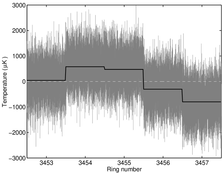
Figure 1: A 5 hour segment of the noise TOD after coadding (grey) and the baselines (black) fitted to it. For this figure the 5-hour average is subtracted also, to center the figure at 0 $\mu$K. The baselines were obtained using the weight function $w=1/n_{p}$. The difference between baselines obtained with different methods would be too small to show up clearly in this figure.

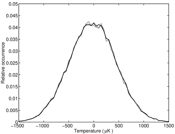
Figure 2: The histogram (in bins of 50 $\mu$K) of the baselines from a set of 10 simulated 7-month noise TODs. The three curves correspond to two different weight functions (see Sect. 3.2) used to determine the baselines: $w=1/n_{p}$ (thick black) and $w=1$ (thin black), and to the reference baselines, i.e., noise averages over the one hour ring (grey).

There was no foreground included in the simulations presented in this paper, but we have also verified our destriping codes on simulated data sets with foreground. We found that the foreground has an insignificant impact on the baselines determined by the destriping, in agreement with the discussion in Maino et al. (Maino02 (2002)). The quality of destriping is also almost independent of the impact of another class of instrumental systematic effects, main beam distortions and straylight, as the temperature differences at crossing pixels are dominated by the noise and only minimally affected by the spurious signals ($\approx\mu$K) introduced by optical distortions (see e.g. Burigana et al. 2001).

Fig. 3 shows the input $C_{\ell}$ spectrum and the spectrum derived from the simulated TOD after destriping. We used the Anafast code of the HEALPix package to compute the $C_{\ell}$ spectrum of the destriped map. We subtracted from the derived spectrum an estimate of the noise level $C_{\rm noise}=0.197\mu{\rm K}^{2}$ (estimated as the average of $C_{\ell}$ over $\ell=980\ldots 1000$) and corrected the spectrum for the beam shape convolution and pixel convolution. The angular spectrum shown is thus $\tilde{C}_{\ell}=(C_{\ell}-C_{\rm noise})/(B^{2}_{\ell}h^{2}_{\ell})$, where $B_{\ell}=\exp(-\sigma_{b}^{2}\ell(\ell+1)/2)$, with $\sigma_{b}=10^{\prime}/\sqrt{8\ln(2)}$, is the beam convolution function corresponding to the assumed beam width of $10^{\prime}$ (FWHM), and $h_{\ell}$ is the pixel convolution function (provided by the HEALPix package).

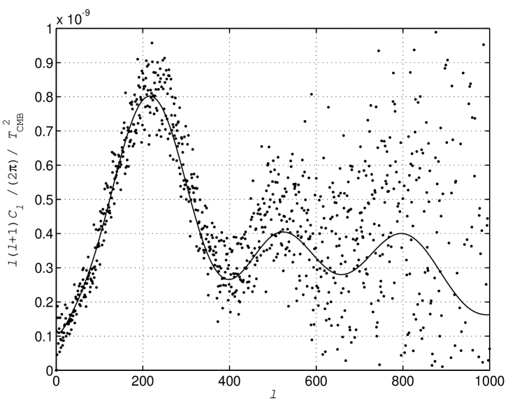
Figure 3: The input $C_{\ell}$ spectrum and the spectrum computed from the CMB map. The latter has been corrected for beam and pixel convolution, and for white noise level. Destriping was done fitting uniform baselines only.

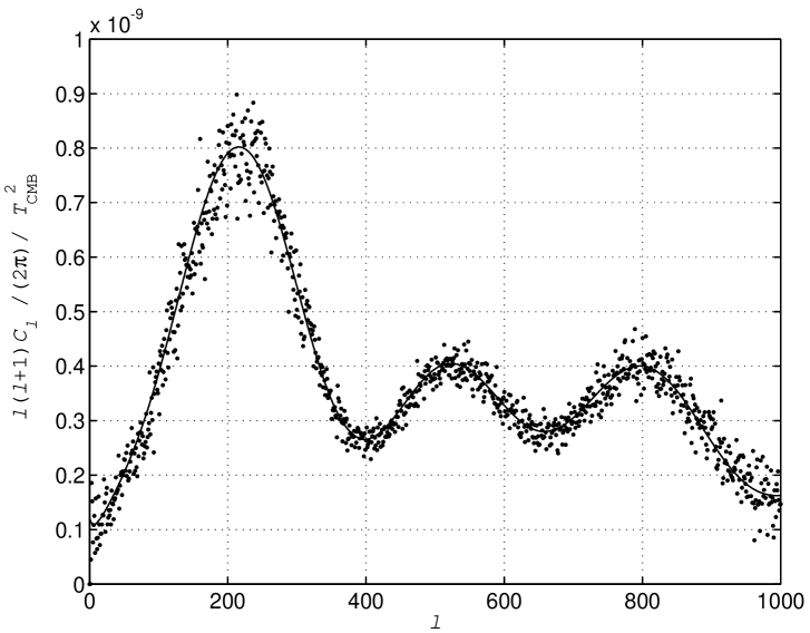
Figure 4: Same as Fig. 3, but for noise level lowered by factor $1/\sqrt{24}$. This simulates the effect of combining 24 detectors.

Fig. 4 shows the same for a noise level reduced by the factor $\sqrt{24}$, corresponding to the combination of 24 detectors. Here the subtracted noise level was $C_{\rm noise}=0.197\mu{\rm K}^{2}/24=0.0082\mu{\rm K}^{2}$.

Note that Figs. 3 and 4 are for illustration only, as this paper does not address the full CMB $C_{\ell}$ estimation problem, and thus we have just used the above crude estimate for $C_{\mathrm{noise}}$.

3.2 Comparison of different weighting schemes: maps and angular power spectra

We have written a destriping code which allows us to compare the different weight functions discussed in Sect. 2.3. We use the Cholesky decomposition technique to solve the set of linear equations.

We have chosen the root-mean-square (rms) value of the residual noise map (see below) pixels as a figure of merit that we use to compare different destriping methods. This map rms is related to the $C_{\ell}$ spectrum through the relation

$${\rm rms}^{2}=\sum_{\ell}\frac{2\ell+1}{4\pi f_{\rm sky}}C_{\ell}.$$ (18)

The map rms squared is thus a weighted sum of the angular spectrum, with high weight on high multipoles. The sky coverage $f_{\rm sky}=0.985$ enters here because we have computed our rms values over the visited pixels only. When computing $C_{\ell}$ spectra, we have set $T=0$ in the remaining pixels.

We compute the residual noise map by taking the difference between the destriped map and the noise-free reference map and subtracting the monopole component. Note that because of the incomplete sky coverage, removing the monopole affects the $C_{\ell}$ spectrum at all $\ell$ (not only $\ell=0$). The reference map is computed by coadding the pure signal TOD into a map of resolution $N_{\rm side}$=512. The expected contribution from white noise to the residual map rms is 220.95 $\mu$K.

While the rms of the residual noise map is a natural measure of the CMB map quality, the main scientific interest is perhaps not in the CMB map itself, but rather in its angular power spectrum $C_{\ell}$. It is therefore of interest to see the impact of the destriping methods on the different parts of the $C_{\ell}$ spectrum. The map rms is dominated by the high $\ell$ part, and does not reveal the difference in performance of the various methods in the low $\ell$ part. Thus we have computed the angular power spectra $C_{\ell}$ of the residual noise maps.

Because of the random nature of the noise, the result of a comparison between methods may vary from one noise realization to another. We therefore performed destriping 10 times, with different realizations of instrument noise. The underlying CMB map was kept the same. We then used the average of the 10 residual map rms values and the residual noise map $C_{\ell}$ spectra to compare the methods. We also calculated the standard deviation (std) of the 10 map rms and $C_{\ell}$ values, to see whether the differences between the methods were statistically significant. Thus this average rms approximates the expectation value for the rms with an accuracy of $\mbox{std}/\sqrt{10}$. However, the std itself tells us how much we can expect the residual map rms for a single realization to deviate from this average value.

Table 1 presents a comparison between different weight functions discussed in Sect. 2.3. The corresponding $C_{\ell}$ spectra are shown in Fig. 5. Since from our simulations we have the noise streams available separately, we also computed reference baselines as the average of the noise stream over each ring. This reference baseline can be thought of as the “true” baseline of the noise. For comparison, we then subtracted the reference baselines from the TOD and computed the rms of the resulting map. This represents an ideal situation, where we could determine the baselines exactly. The reference rms is given on the last line of Table 1. Actual residual noise rms values are always larger.

Weight functions $w=1/n_{p}$ and $w=1/(n_{p}-1)$ in Eq. (16) give similar results, due to the fact that for most pixels $n_{p}\gg 1$. Weight $w=1/n_{p}$ suggested by our maximum likelihood analysis is clearly superior to $w=1$. However, the weight $w=1/(n_{p}-1)$ gives an even smaller rms, although the difference is very small. The difference of the rms between $w=1$ and $w=1/n_{p}$ is significant because the difference is about 10 times larger than the respective std of the rms. Although the difference between $w=1/n_{p}$ and $w=1/(n_{p}-1)$ is much less than the std between different noise realizations, it was in the same direction in each realization. Note that we were able to measure this small difference only because we used the same set of random seeds for all weighting schemes.

Table 1: Average (avg) rms and std of rms of the residual noise map for different weight functions. The average and std are taken over 10 noise realizations. The corresponding $C_{\ell}$ spectra are shown in Fig. 5. The last line gives the reference rms, which would be reached if one could determine the baselines exactly. The differences between the rms are significant only if they are larger than the std. We show extra digits for the rms in Tables 1 and 2 to show the systematic (but insignificant) difference (see text) between the $w=1/(n_{p}-1)$ and $w=1/n_{p}$ cases.

Weight	avg rms$/\mu$K	std of rms$/\mu$K
$w=1$	225.1619	0.072
$w=1/(n_{p}-1)$	224.4332	0.073
$w=1/n_{p}$	224.4443	0.073
ref.	224.1170	0.075

Table 2: Average rms and std of rms of the residual noise map, for a simplified noise model. The noise consists of uniform baselines + white noise.

Weight	avg rms$/\mu$K	std of rms$/\mu$K
$w=1$	221.4816	0.069
$w=1/(n_{p}-1)$	221.1041	0.072
$w=1/n_{p}$	221.1039	0.072
ref.	220.9593	0.073

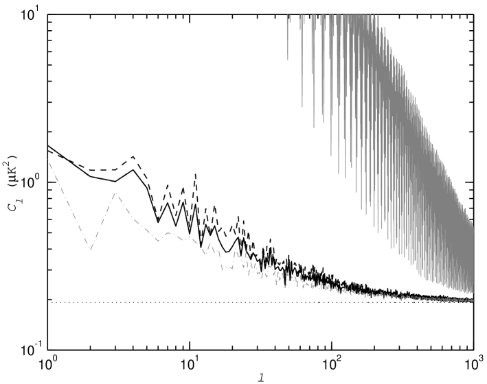
Figure 5: The $C_{\ell}$ spectrum of the residual noise map, for different choices of the weight function $w$. The spectra are averages over 10 realizations of noise. Only uniform baselines are fitted. The lower solid line corresponds to the choice $w=1/n_{p}$ for the weight function in Eq. (16) and the dashed line to $w=\mbox{const}$. The difference between weight functions $w=1/n_{p}$ and $w=1/(n_{p}-1)$ is too small to show on this plot. The difference between them is plotted in Fig. 6 (lower panel). The upper solid (gray) line shows the spectrum of a naive coadded map (no destriping). The dash-dotted (gray) line shows the ideal reference spectrum, computed by removing the reference baselines. The corresponding map rms values are shown in Table 1. The dotted line shows the theoretical white noise level $0.192\mu{\rm K}^{2}$.

Since the difference between the weight functions $w=1/n_{p}$ and $w=1/(n_{p}-1)$ is so small that it does not show up in Fig. 5, we show just the differences in Fig. 6.

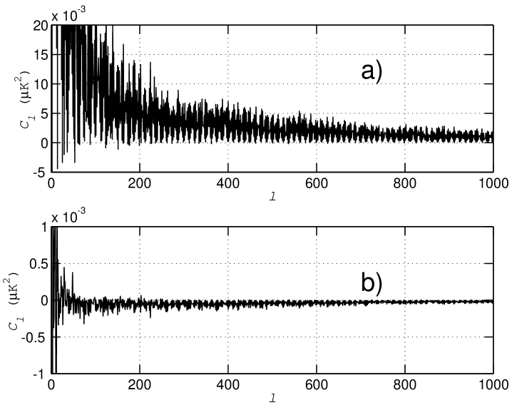
Figure 6: Differences between the $C_{\ell}$ spectra shown in Fig. 5. a) The difference $C_{\ell}(w=\mbox{const})-C_{\ell}(w=1/n_{p})$. b) The difference $C_{\ell}(w=1/(n_{p}-1))-C_{\ell}(w=1/n_{p})$. Note the much expanded vertical scale in Fig. 6b.

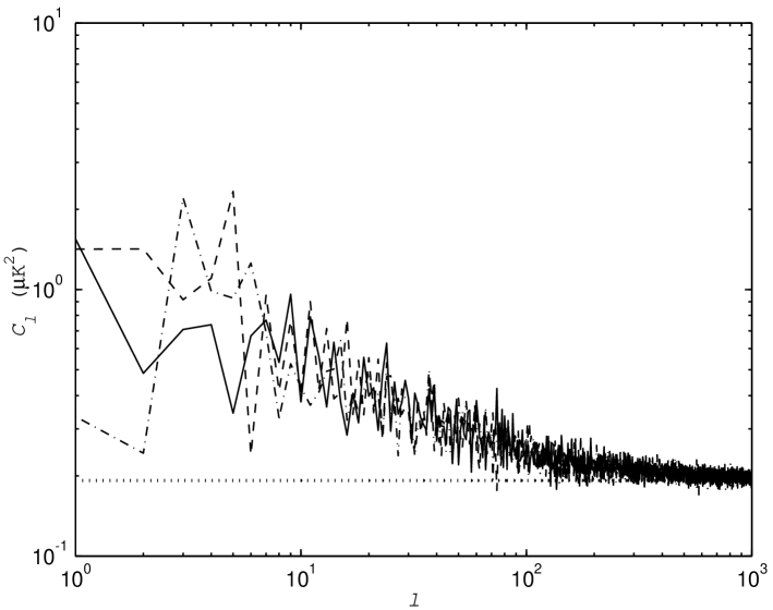
Figure 7: Three examples of individual $C_{\ell}$ spectra, from different noise realizations, after destriping. Only uniform baselines are fitted. The average of 10 such spectra is shown in Fig. 5 (the solid line there).

It is well known that maximum-likelihood analysis should provide the minimum-variance solution. Therefore it may at first seem surprising that the maximum-likelihood based weight function did not give the best results. However, the maximum-likelihood solution is the optimal one only if the model used corresponds to reality. Here we have modelled the $1/f$ noise component in the TOD by a uniform baseline, which is a simplified model. Further, we have assumed that the baselines are independent from ring to ring. The reason for the maximum-likelihood solution not giving the best result is that the noise model used in the analysis does not exactly correspond to the actual noise properties.

To verify this, we re-generated our input noise in a way that better corresponds to the model assumed in the analysis. We generated the $1/f$ noise in the usual way, but then, for each ring, we took the average over the ring, and replaced the original $1/f$ contribution to the ring with this average value, on top of which we added white noise. This way we obtained noise which still has a realistic correlation between scanning rings, but consists of baselines + white noise only. The results are shown in Table 2. Now the maximum-likelihood based weight function gives the smallest variance map.

Thus it seems that the slightly better performance of the Delabrouille weighting scheme ($w=1/(n_{p}-1)$) is related to the effect of that part of the correlated noise which deviates from uniform baselines.

The scatter in the individual residual noise map $C_{l}$ values from one noise realization to another was larger than the difference between the methods. (See Fig. 7 for the $C_{\ell}$ spectra from the first three noise realizations, using our weighting scheme, $w=1/n_{p}$.) The difference between $w=1$ and $w=1/n_{p}$ becomes however statistically significant when the $C_{\ell}$ are binned into larger bins.

4 Increasing the number of base functions

As shown by Delabrouille (Delabrouille98 (1998)) and Maino et al. (Maino99 (1999, 2002)), a simple model with uniform baselines and white noise models quite well the coadded noise stream. One can try to further improve the performance of destriping by introducing more base functions. Delabrouille (Delabrouille98 (1998)) found that the addition of a small number of base functions improved the performance of destriping, whereas Maino et al. (Maino02 (2002)) found no significant improvement. The difference between these results could be due to the different noise spectra considered: $1/f$ noise for Maino et al. (Maino02 (2002)) and $1/f^{2}$ for Delabrouille (Delabrouille98 (1998)).

We generalize the discussion of Sect. 2 to include arbitrary base functions. We model the correlated noise component of the TOD by a linear combination of base functions as ${\bf n}_{\rm corr}=\mathbf{F}{\bf a}$. Here $\mathbf{F}$ is a matrix, whose columns contain the base functions, and ${\bf a}$ is a vector containing their (unknown) amplitudes. It is convenient to select an orthogonal set of the base functions, so that $\mathbf{F}^{T}\mathbf{F}$ is diagonal. Eqs. (5)–(13) hold as such for general baselines.

We have studied two sets of base functions: Fourier components and Legendre polynomials. Both form an orthogonal set.

4.1 Simulation results

The solution of the general destriping problem involves the solution of a large linear system of equations

$$\mathbf{F}^{T}\mathbf{Z}\mathbf{F}{\bf a}=\mathbf{F}^{T}\mathbf{Z}{\bf y}.$$ (19)

Matrix $\mathbf{A}\equiv\mathbf{F}^{T}\mathbf{Z}\mathbf{F}$ becomes very large if several base functions are fitted. We use the iterative conjugate gradient method (see, e.g., Press et al. NumRes (1992)) to solve the system. The conjugate gradient method only requires multiplication by matrix $\mathbf{A}$. That can easily be done algorithmically, without actually storing the full matrix $\mathbf{A}$ at any one time. The conjugate gradient method allows us to perform the destriping in a relatively small memory space.

Note that we do not need to add the term ${\bf 1}{\bf 1}^{T}$, since the conjugate gradient method has the property that, when solving system $\mathbf{A}{\bf x}={\bf b}$, it automatically finds the solution for which ${\bf x}_{0}^{T}{\bf x}=0$, if iteration is started with ${\bf x}=0$, and $\mathbf{A}{\bf x}_{0}=0$ and ${\bf b}^{T}{\bf x}_{0}=0$. (The amplitude vector which gives unit amplitudes to the uniform baselines and zero amplitudes to other baselines is an example of such a vector ${\bf x}_{0}$, so the average of the uniform baselines is set to zero. The case of other possible vectors in the null space of $\mathbf{A}$ is discussed further below.)

We compare four sets of functions:
1. (“Un.”) Uniform baselines only.
2. (“F1”) Uniform baseline + first Fourier frequency, which gives three components for each ring: constant, $\sin(2\pi f_{\rm sc}t)$, and $\cos(2\pi f_{\rm sc}t)$ ($q=0,1,2$). Here $f_{\rm sc}=1/$(60 s) is the scanning frequency.
3. (“L1”) Uniform baseline + 1st (linear) Legendre polynomial.
4. (“L2”) Uniform baseline + 1st and 2nd Legendre polynomials.

The first Legendre polynomials are $L(x,0)=1$, $L(x,1)=x$, and $L(x,2)=\frac{1}{2}(3x^{2}-1)$, for $x\in[-1,1]$.

Again we averaged the residual noise $C_{\ell}$ spectra and the residual noise map rms over 10 noise realizations.

Table 3 and Fig. 8 present our results of fitting several base functions. We find no improvement in the map rms.

The last column of Table 3 gives a reference rms, which was computed as follows. We defined the reference amplitude vector as ${\bf a}_{0}=(\mathbf{F}^{T}\mathbf{F})^{-1}\mathbf{F}^{T}{\bf n}$, where ${\bf n}$ is the pure noise stream (i.e. ${\bf n}_{\rm corr}+{\bf n}$ of Eq. (4). We coadded a map from the TOD stream, from which we had removed the reference base functions, ${\bf y}-F{\bf a}_{0}$, and computed the rms of the residual noise map. Fourier components give the lowest reference rms, showing that Fourier components model the noise best of our base function sets. However, when we fit the data, Fourier components give the poorest results, as the first column of Table 3 shows. The worst of the 10 runs gave a rms of 452 $\mu$K. The code took a long time to converge, and the final maps contained a very strong and obviously unphysical dipole-like structure. (The large std in the case of Fourier components does not mean that for some realizations the Fourier components would have given a lower rms than the other methods. Rather, the distribution was just very skew; a small number of realizations gave a very large rms, but all 10 realizations gave an rms larger than the average for any of the other methods.)

The problem with Fourier components is related to small eigenvalues of matrix $\mathbf{A}$. If there exists a map ${\bf m}^{\prime}$ such that

$$\mathbf{P}{\bf m}^{\prime}=\mathbf{F}{\bf a}^{\prime}$$ (20)

for some ${\bf a}^{\prime}$, then ${\bf a}^{\prime}$ is an eigenvector of $\mathbf{A}$ with zero eigenvalue. If ${\bf a}$ is a solution of Eq. (19), then ${\bf a}+{\bf a}^{\prime}$ is also a solution. In other words, if we can produce the same TOD stream both as a combination of the base functions, and by picking it from a map with our scanning strategy, then it is not possible, without further information, to tell if this TOD component comes from noise or signal. In practice zero eigenvalues are unlikely to happen, but already small but non-vanishing eigenvalues cause similar problems. Eq. (20) then holds approximatively.

The difficulty of fitting Fourier components is related to the symmetry of the nominal scanning strategy of Planck. Suppose the scanning rings are regular circles with centers on the ecliptic plane. If we give all cosine and sine components equal amplitudes $a$ and $b$ such that the resulting function $a\cos\phi+b\sin\phi$ ($\phi$ runs from $0$ to $2\pi$ around the ring) is at maximum at the northernmost point and at minimum at the southernmost point (or vice versa), and coadd a map from this TOD stream, we obtain a meridian symmetric map for which relation (20) holds. This noise component cannot be resolved without further information on noise properties. The same problem also affects fitting 2nd order Legendre polynomials, albeit less severely. We would expect that other, less symmetric, scanning strategies would not be as prone to such problems.

We discuss this problem quantitatively in the following.

Table 3: Average rms (in $\mu$K) of the residual noise map, std of rms, and reference rms, for different sets of base functions. The reference rms is computed from a map from which the reference baseline functions are removed. The base functions were: Un: uniform baseline, F1: three Fourier modes, L1 (L2): Legendre polynomials up to 1st (2nd) order. The two first lines (’Un.’) represent the same destriping methods as the first and third lines of Table 1.

fit	avg rms$/\mu$K	std of rms/$\mu$K	ref. rms/$\mu$K
Un. ($w=1$)	225.162	$\pm$ 0.072	224.117
Un. ($w=1/n_{p}$)	224.444	$\pm$ 0.073	224.117
F1	264.131	$\pm$70.460	223.621
L1	224.463	$\pm$ 0.077	223.860
L2	225.049	$\pm$ 0.463	223.748

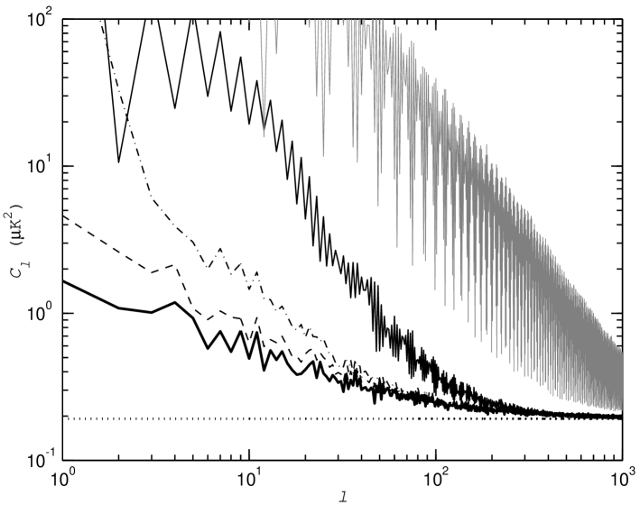
Figure 8: Average $C_{\ell}$ spectrum of the residual noise map, for different choices of the base functions. Thick solid line: uniform baselines. Thin solid lower line: three Fourier components ($q=0,1,2$). Dashed and dot-dashed lines: Legendre polynomials up to 1st and 2nd order. The upper solid (gray) line shows the spectrum of a naive coadded map (no destriping). The spectra were averaged over 10 realizations of noise.

4.2 Eigenvalue analysis of the destriping problem

Consider the solution of Eq. (19) in light of eigenvalue analysis.

Assume the TOD stream is of the form

$${\bf y}=\mathbf{P}{\bf m_{0}}+\mathbf{F}{\bf a}_{0}+{\bf n}$$ (21)

where ${\bf m}_{0}$ is the actual map, ${\bf a}_{0}$ is the “true” baseline vector, and ${\bf n}$ represents the remaining noise component. With these assumptions, Eq. (19) becomes

$$\mathbf{F}^{T}\mathbf{Z}\mathbf{F}{\bf a}=\mathbf{F}^{T}\mathbf{Z}\mathbf{F}{\bf a}_{0}+\mathbf{F}^{T}\mathbf{Z}{\bf n}.$$ (22)

Let $\lambda_{i}$ and ${\bf u_{i}}$ be the eigenvalues and corresponding orthonormal eigenvectors of matrix $\mathbf{A}=\mathbf{F}^{T}\mathbf{Z}\mathbf{F}$. Because $\mathbf{A}$ is symmetric and non-negative definite, all eigenvalues are positive or zero, $\lambda_{i}\geq 0$, and the eigenvectors form a complete orthogonal basis. The matrix can be presented by its eigenvectors as

$$\mathbf{F}^{T}\mathbf{Z}\mathbf{F}=\sum_{i}\lambda_{i}{\bf u}_{i}{\bf u}_{i}^{T}.$$ (23)

We can expand ${\bf a}=\sum_{i}a_{i}{\bf u}_{i}$ and ${\bf a}_{0}=\sum_{i}a_{i}^{0}{\bf u}_{i}$ and

$$\mathbf{F}^{T}\mathbf{Z}{\bf n}=\sum_{i}c_{i}{\bf u}_{i}.$$ (24)

We substitute these expansions into (22) to find

$$a_{i}=a_{i}^{0}+c_{i}/\lambda_{i}.$$ (25)

Here it must be understood that this relation holds for components for which $\lambda_{i}>0$. For $\lambda_{i}=0$ one can easily show that $c_{i}=0$ and $a_{i}$ remains undefined.

Consider then the statistical properties of coefficients $c_{i}$. Since $c_{i}={\bf u}_{i}^{T}\mathbf{F}^{T}\mathbf{Z}{\bf n}$, we find, assuming that ${\bf n}$ is white and $\langle{\bf n}{\bf n}^{T}\rangle=diag(\sigma^{2})$, that $\langle c_{i}\rangle=0$ and

$$\langle c_{i}c_{k}\rangle=\sigma^{2}{\bf u}_{i}^{T}\mathbf{F}^{T}\mathbf{Z}\mathbf{F}{\bf u}_{k}=\sigma^{2}\lambda_{i}\delta_{ik}.$$ (26)

Looking back at Eq. (25) we observe that

$$\langle(a_{k}-a_{k}^{0})(a_{i}-a_{i}^{0})\rangle=\frac{\sigma^{2}}{\lambda_{i}}\delta_{ik}.$$ (27)

We see that if one of the eigenvalues is very small, then the inaccuracy in the corresponding component $a_{i}$ is very large. Actually, the vanishing eigenvalues do not pose a problem, since the conjugate gradient algorithm always sets the corresponding amplitude to zero. Problems are caused by moderately small, but non-vanishing, eigenvalues. How small a value must be regarded as zero depends on the floating point accuracy of the computer and on the convergence criterion one has chosen for the conjugate gradient algorithm.

We have seen that fitting uniform baselines only already gives good results.There is no advantage in trying to fit additional components which have a large inaccuracy. Fitting poorly determined components causes more error than leaving them out entirely. We therefore aim to fit only components that correspond to a large eigenvalue, and eliminate small eigenvalue components. In the following we present a practical method to do this. The method presented does not require full determination of eigenvalues or eigenvectors of matrix $\mathbf{A}$, which would be a computationally expensive task.

4.3 A practical method

Consider the following equation:

$$(\mathbf{F}^{T}\mathbf{Z}\mathbf{F}+\epsilon\mathbf{F}^{T}\mathbf{F}){\bf a}=\mathbf{F}^{T}\mathbf{Z}{\bf y}$$ (28)

where $\epsilon$ is a small positive constant. An eigenvalue analysis similar to that presented above shows that the solution of Eq. (28) is related to the solution of (19) through

$$a_{i}^{\prime}=a_{i}\frac{\lambda_{i}}{\lambda_{i}+\epsilon\lambda_{max}},$$ (29)

where $\lambda_{max}$ is the largest possible eigenvalue of $\mathbf{A}$. With our chosen normalization $\mathbf{F}^{T}\mathbf{F}=diag(n_{b})$ it is equal to the number of samples on a ring, $\lambda_{max}=n_{b}$.

The effect of the $\epsilon$ term in Eq. (28) is to wash out components with eigenvalues smaller than $\epsilon\lambda_{max}$, while the large eigenvalue component remains unaffected, as long as $\epsilon$ is small. At the limit $\epsilon\rightarrow 0$ the solution of Eq. (28) approaches that of Eq. (19).

We have repeated our computations with this method. Table 4 presents our results for different values of $\epsilon$. The results were again obtained using 10 different realizations of the instrument noise, over which the average and the standard deviation were calculated. We see that, with values $10^{-6}\leq\epsilon\leq 10^{-3}$, the accuracy of fitting Fourier components is strongly improved with respect to the $\epsilon=0$ case. Also the required computation time is reduced. For 2nd order Legendre polynomials we also find a clear improvement.

However, the results for multiple base functions are still worse than for uniform baselines only.

Uniform baselines and 1st order Legendre polynomials, which exhibited no problems with $\epsilon=0$, are unaffected with $\epsilon=10^{-4}$ or less, but with $\epsilon=10^{-3}$ or larger the accuracy of fitting them begins to deteriorate.

Fig. 9 shows the residual noise $C_{\ell}$ spectra for the $\epsilon=10^{-4}$ case.

Depending on the number of base functions, the code took 3-5 seconds per iteration step on one processor of an IBM eServer Cluster 1600 computer. The total computation time varied between 2 and 30 minutes.

Table 4: Average rms (in $\mu$K) of the residual noise map, std of rms (middle), and number of iteration steps for different sets of base functions and for different values of $\epsilon$ ($f_{k}=0.1$ Hz). The last line gives the reference rms. Parameter $\epsilon$ is defined in Eq. (28). The base functions were: Un: uniform baseline, F1: three Fourier modes, L1 (L2): Legendre polynomials up to 1st (2nd) order.

$\epsilon$	Un.	F1	L1	L2
rms
$0$	224.444	264.131	224.463	225.049
$10^{-7}$	224.444	251.648	224.463	225.047
$10^{-6}$	224.444	229.675	224.463	225.025
$10^{-5}$	224.444	226.034	224.463	224.866
$10^{-4}$	224.444	225.640	224.463	224.563
$10^{-3}$	224.463	225.438	224.502	224.678
$10^{-2}$	226.192	230.141	227.691	230.396
ref.	224.117	223.621	223.860	223.748
std of rms
$0$	0.073	70.460	0.077	0.463
$10^{-7}$	0.073	48.449	0.077	0.461
$10^{-6}$	0.073	7.044	0.077	0.445
$10^{-5}$	0.073	0.450	0.077	0.327
$10^{-4}$	0.073	0.168	0.077	0.109
$10^{-3}$	0.072	0.196	0.078	0.130
$10^{-2}$	0.230	0.803	0.491	1.311
Iteration steps
$0$	28	373	39	130
$10^{-7}$	28	369	39	130
$10^{-6}$	28	351	39	130
$10^{-5}$	28	318	39	128
$10^{-4}$	28	166	38	119
$10^{-3}$	27	102	37	95
$10^{-2}$	25	46	31	47

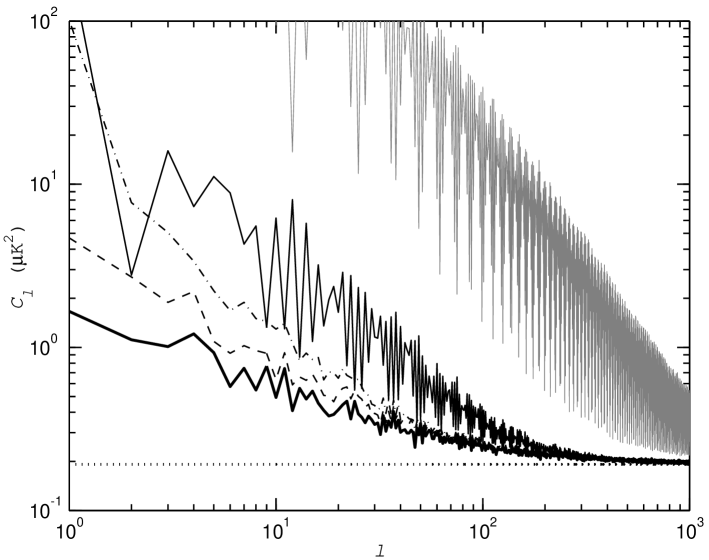
Figure 9: Same as Fig. 8, but for the improved method with $\epsilon=10^{-4}$. Thick solid line: uniform baselines. Thin solid lower line: three Fourier components ($q=0,1,2$). Dashed and dot-dashed lines: Legendre polynomials up to 1st and 2nd order. The corresponding map rms values are shown in Table 4.

To illustrate the use of several base functions we show in Fig. 10 the same 5 hour coadded noise TOD as in Fig. 1, but now with different sets of base functions. Note that the deviations from uniform baselines are exaggerated in this figure. The actual amplitudes of the other base functions are much smaller (by about a factor of 20) than those of the uniform components.

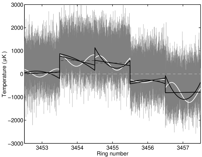
Figure 10: Same as Fig. 1, but now with different sets of base functions. The amplitudes of the other base functions were much smaller than the uniform components, so that it would be difficult to see the small deviation from uniform baselines. Therefore we have exaggerated the deviation from the uniform-baseline case by a factor of 5 in this figure. Dashed line: uniform baselines. White solid line: three Fourier components ($q=0,1,2$). Black solid lines: Legendre polynomials up to 1st and 2nd order.

In order to check how the results depend on the knee frequency, we repeated our computations with rescaled noise. We took the $1/f$ noise stream, which was originally generated with $f_{\mathrm{k}}=0.1$ Hz, scaled it by a factor 0.5 or 2, and added white noise with the same variance in all cases. This is equivalent to changing the knee frequency by a factor of 0.25 or 4. We thus have results for three knee frequencies: $f_{k}=0.025$Hz, $f_{\mathrm{k}}=0.1$Hz, and $f_{\mathrm{k}}=0.4$Hz.

The obtained residual map rms for $f_{k}=0.4$Hz and $f_{\mathrm{k}}=0.025$Hz are shown in Tables 5 and 6, for different values of $\epsilon$. The optimal value of $\epsilon$ seems to depend somewhat on knee frequency, being smaller at higher knee frequencies.

The $C_{\ell}$ spectra for $\epsilon=10^{-4}$ for knee frequencies $f_{\mathrm{k}}=0.1\mbox{Hz}$, $f_{\mathrm{k}}=0.4\mbox{Hz}$, and $f_{\mathrm{k}}=0.025\mbox{Hz}$ are shown in Figs. 9, 11, 12, respectively. The std of the $C_{\ell}$ for the $f_{\mathrm{k}}=0.1\mbox{Hz}$ case are shown in Fig. 14.

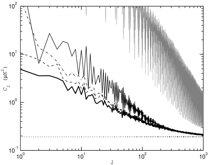
Figure 11: Same as Fig. 9 but for knee frequency $f_{\mathrm{k}}=0.4$Hz.

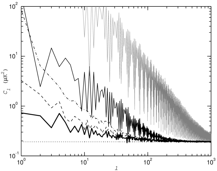
Figure 12: Same as Fig. 9 but for knee frequency $f_{\mathrm{k}}=0.025$Hz.

Looking at the average $C_{\ell}$ spectra of residual noise and their std we see that fitting additional base functions decreases the accuracy of destriping at low $\ell$. However the situation for the map rms values in Table 5 seems more complicated. For $f_{\mathrm{k}}=0.1\mbox{Hz}$ or smaller, fitting additional base functions does not improve the performance of destriping, but with $f_{\mathrm{k}}=0.4\mbox{Hz}$ fitting one or two Legendre polynomials besides the constant baselines decreases the map rms, while Fourier components still give inferior results. The improvement in the map rms for $f_{\mathrm{k}}=0.4\mbox{Hz}$, when fitting Legendre polynomials, comes from the high multipoles. This can be seen from Fig. 13, where we plot the difference between the residual noise $C_{\ell}$ obtained when fitting Legendre polynomials or Fourier components, and when fitting uniform baselines only.

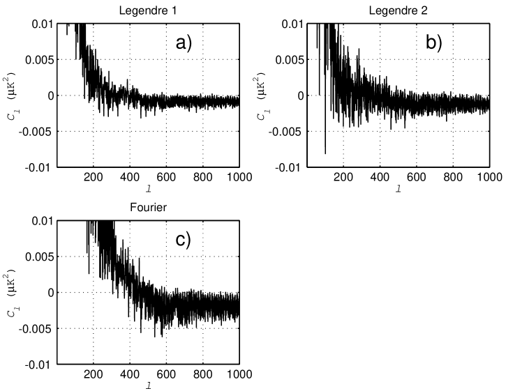
Figure 13: Differences between $C_{\ell}$ spectra shown in Fig. 11 ($f_{\mathrm{k}}=0.4\mbox{Hz}$). The three panels show the change in the $C_{\ell}$ spectrum when fitting Legendre polynomials up to a) 1st or b) 2nd order, or c) three Fourier components, instead of uniform baselines only.

We see that increasing the number of base functions improves the high $\ell$ but worsens the low $\ell$ part of the $C_{\ell}$ spectra. This is true both for Fourier components and for Legendre polynomials. This trend persists for lower $f_{\mathrm{k}}$, but the value of $\ell$ above which we get an improvement goes up and the improvement for those $\ell$ becomes smaller.

Delabrouille (Delabrouille98 (1998)) obtained improved results by fitting several base functions already with $f_{\mathrm{k}}=0.1\mbox{Hz}$. The difference between our results and his is probably due to differences in the noise model. While we assume $P\propto f^{-1}$, as appropriate for LFI radiometers (Seiffert et al. Seiffert02 (2002)), Delabrouille assumes a noise spectrum of the form $P\propto f^{-2}$ to account also for possible thermal fluctuations and atmospheric noise in ground based and balloon borne bolometer experiments. This leads to more low-frequency noise for a given knee frequency.

The std of the residual noise $C_{\ell}$ influences the accuracy at which the $C_{\ell}$ spectrum of the CMB can be estimated from the noisy data. From Fig. 14 we can see that at low $\ell$ uniform baselines give the best performance in the sense that the $C_{\ell}$ of the residual noise varies the least from one realization to another. At high $\ell$ there is no clear difference between the performances of different sets of base functions.

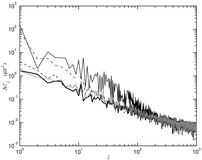
Figure 14: Standard deviation (std) of the residual noise $C_{\ell}$ over 10 noise realizations, for different choices of the base functions ($f_{k}=0.1$ Hz, $\epsilon=10^{-4}$). Thick black line: uniform baselines with $w=1/n_{p}$. Grey line: uniform baselines with $w=1$. Thin solid line: three Fourier components ($q=0,1,2$). Dashed and dot-dashed lines: Legendre polynomials up to 1st and 2nd order. The corresponding map rms and std of map rms values are shown in Table 4.

Table 5: Average rms of the residual noise map (in $\mu$K), for different sets of base functions and for knee frequency $f_{k}=0.4$ Hz. The base functions were: Un: uniform baseline, F1: three Fourier modes, L1 (L2): Legendre polynomials up to 1st (2nd) order. The last line gives the reference rms. The corresponding $C_{\ell}$ spectra for $\epsilon=10^{-4}$ are shown in Fig.11.

$\epsilon$	Un.	F1	L1	L2
$0$	234.184	258.343	233.947	234.544
$10^{-6}$	234.184	238.107	233.947	234.512
$10^{-5}$	234.183	235.603	233.947	234.304
$10^{-4}$	234.183	235.315	233.947	233.910
$10^{-3}$	234.252	235.643	234.102	234.514
ref.	233.337	231.626	232.430	232.045

Table 6: Same as Table 5, but for $f_{k}=0.025$ Hz. The corresponding $C_{\ell}$ spectra for $\epsilon=10^{-4}$ are shown in Fig.12.

$\epsilon$	Un.	F1	L1	L2
$0$	221.943	262.149	222.030	222.597
$10^{-5}$	221.943	223.588	222.030	222.433
$10^{-4}$	221.943	223.173	222.030	222.163
$10^{-3}$	221.948	222.825	222.038	222.149
$10^{-2}$	222.385	223.676	222.835	223.565
ref.	221.753	221.575	221.665	221.626

5 Conclusions

We have presented a maximum-likelihood formulation of the destriping approach to the CMB map-making problem, and a rigorous derivation of the destriping algorithm, and we have applied it to the case of the Planck mission.

We have formulated the method in matrix form, which allows us to apply the conjugate gradient technique in such a way that we can handle very large data sets.

We have compared the three different destriping methods, the one derived here and the other two already presented in the literature, using simulated Planck data (one 100 GHz LFI detector). The differences between these methods can be expressed in terms of a weight function, which varies between methods. This function assigns weights to pixels based on the number of observations falling on that pixel.

We found that our new method provides some improvement to the method used in Burigana et al. (Burigana99 (1997)) and Maino et al. (Maino99 (1999, 2002)). However, our new method was not better than the method given by Delabrouille (Delabrouille98 (1998)), although he gives only a heuristic justification for his weight function. The difference between the latter two methods was insignificantly small, but was systematic. That the maximum-likelihood derivation did not lead to the optimal method in practice is due to actual noise properties differing from the idealization used in the derivation. We recommend using either the weight function derived here ($w=1/n_{p}$) or the one given by Delabrouille ($w=1/(n_{p}-1)$).

We have tested the possibility of improving the accuracy of destriping by fitting more base functions besides the uniform baseline, but we have found no systematic improvement in the case of instrumental $1/f$ noise. (Fitting several base functions may be more beneficial when removing other types of systematics, i.e. periodic fluctuations induced by thermal instabilities.) The optimal selection of base functions seems to depend on the actual spectrum of the noise, and on which multipoles one is mainly interested in. However, the great virtue of the destriping method is its simplicity: it does not require prior information on the noise spectrum. We lose this advantage if we incorporate information on the noise spectrum into the method.

- (1) Bennett, C., Halpern, M., Hinshaw, G., et al. 2003, ApJS, 148, 1
- (2) Bersanelli, M., Muciaccia, P.F., Natoli, P., Vittorio, N., Mandolesi, N. 1997, A&ASS, 121, 393
- (3) Burigana, C., Malaspina, M., Mandolesi, N., et al. 1997, Int. Rep. TeSRE/CNR, 198/1997, November, [astro-ph/9906360]
- (4) Burigana, C., Natoli, P., Vittorio, N., Mandolesi, N., Bersanelli, M. 2002, Experimental Astronomy, 12/2, 87, 2001
- (5) Burigana, C., Maino, D., Górski, K.M., et al. 2001, A&A, 373, 345
- (6) Cappellini, B., Maino, D., Albetti, G., et al. 2003, A&A, 409, 375
- (7) Challinor, D., Mortlock, D.J., van Leeuwen, F., et al. 2002, MNRAS, 331, 994
- (8) Delabrouille, J. 1998,A&ASS, 127, 555
- (9) Górski, K.M., Hivon, E., & Wandelt, B.D. 1999, in Proceedings of the MPA/ESO Cosmology Conference ”Evolution of Large-Scale Structure”, ed. A.J. Banday, R.S. Sheth, & L. Da Costa, PrintPartners Ipskamp, NL, 37, [astro-ph/9812350]
- (10) Maino, D., Burigana, C., Maltoni, M., et al. 1999, A&ASS, 140, 383
- (11) Maino, D., Burigana, C., Górski, K.M., Mandolesi, N., & Bersanelli, M. 2002, A&A, 387, 356
- (12) Mennella, A., Bersanelli, M., Burigana, C., et al. 2002, A&A, 384, 736
- (13) Natoli, P., De Gasperis, G., Gheller, C., Vittorio, N. 2001, A&A, 372, 346
- (14) Piat, M., Lagache, G., Bernard, J.P., Giard. M., Puget, J.L. 2003, A&A, 393, 359
- (15) Press, W.H., Teukolsky, S.A., Wetterling, W.T., & Flannery, B.P. 1992, Numerical Recipes, 2nd ed. (Cambridge University Press, Cambridge)
- (16) Seiffert, M., Mennella, A., Burigana, C., et al. 2002, A&A, 391, 1185
- (17) Seljak, U., & Zaldarriaga, M. 1996, ApJ, 469, 437
- (18) Terenzi, L., Bersanelli, M., Burigana, C., et al. 2002, in “Experimental Cosmology at millimeter wavelengths’, Cervinia, Italy, 9-13 July 2001, AIP Conf. Proc. 616, pg. 245, [astro-ph/0203397]
- (19) van Leeuwen, F., Challinor, A.D., Mortlock, D.J., et al. 2002, MNRAS, 331, 975