A Code for Stellar Binary Evolution and its Application to the Formation of Helium White Dwarfs

Abstract

We present a numerical code intended for calculating stellar evolution in close binary systems. In doing so, we consider that mass transfer episodes occur when the stellar size overflows the corresponding Roche lobe. In such situation we equate the radius of the star with the equivalent radius of the Roche lobe. This equation is handled implicitly together with those corresponding to the whole structure of the star. We describe in detail the necessary modifications to the standard Henyey technique for treating the mass loss rate implicitly together with thin outer layers integrations.

We have applied this code to the calculation of the formation of low mass, helium white dwarfs in low mass close binary systems. We found that the global numerical convergence properties are fairly good. In particular, the onset and end of mass transfer episodes is computed automatically.

1 Introduction

Stellar evolution in binary systems is a classical topic of stellar astrophysics. The study of stellar evolution in this kind of systems has great importance, since an important fraction of know stars belong to binary systems. Inasmuch as, if we want to build a stellar evolution theory able to account for the observations, it is essential to study stellar evolution in binary systems.

According to the standard model, the initially most massive star, usually named the primary evolves faster and, as consequence of its nuclear evolution, begin to inflate. If stars are sufficiently close each other (close binary systems, hereafter CBS) the primary will overflow of the “Roche lobe”. This lobe is found by considering the problem of a binary system in which the orbits are circular, and rotation of both objects is synchronized with orbital motion. Therefore we have the Largange solution to the restricted three body problem, considering that each gas particle is of infinitesimal mass. The Roche lobe corresponds to an equipotential surface that surrounds the stars and represents the limiting volume that can be attained by the stars of the pair before the beginning of mass transfer either, onto the companion, and/or outside the system. From this moment on, the evolution of each star is markedly different from the one they would have in isolation.

According to Kippenhahn & Weigert (1967) mass transfer may begin during core hydrogen burning (case A) and also during central contraction after central hydrogen exhaustion (case B). If it begins after core helium burning it is commonly referred to as case C (Lauterborn 1970). Mass transfer can occur in conservative conditions (total mass and orbital angular momentum conserved) or with mass and/or angular momentum losses from the system. These losses can drastically affect the evolution of the star in a CBS. For reviews on stellar evolution in binary systems, see, e.g., Paczyński (1971), Iben (1985), Iben & Livio (1993), and Taam & Sandquist(2000).

In view of the large number of situations that can be encountered, it is not surprising that CBSs are considered as favorable places for the occurrence of a number of phenomenologies with high astrophysical interest: X-ray sources (van der Klis 2002), low mass helium white dwarfs (Kippenhahn, Kohl & Weigert 1967), planetary nebulae with binary nucleus (Iben & Livio 1993), binary radio pulsars (Bhattacharya & van den Heuvel 1991), supernova progenitors (Podsiadlowski, Joss & Hsu 1992). In this last case, binary evolution naturally accounts for the evolution of the progenitor of SN 1987A. This object was a blue supergiant, a fact difficult to explain in the frame of single stellar evolution, but not in binary evolution (Podsiadlowski, et al. 1992).

In view of the importance of this line of research, in our Observatory we have begun the study of CBSs. To this end, we have developed a code to compute stellar evolution in CBSs, including the self consistent calculation of the mass transfer rate $\dot{M}$ (hereafter MTR). The main purpose of the present paper is to describe the numerical techniques employed in our program for the computation the evolution of stars in a CBS. This code is based on a modification of the Henyey technique presented in Kippenhahn, Weigert & Hofmeister (1967) to solve the set of difference equations of stellar evolution with the inclusion of hydrodynamical effects and the MTR. As a first application of this new code to the case of CBSs that lead to the formation of helium white dwarfs.

As stated above, the main characteristic of our code is that, during mass transfer episodes, it finds the MTR in a fully implicit way by means of a single iterative procedure. This is in contrast with the usual procedure employed by other researchers (see, e.g., Podsiadlowski, Rappaport, & Pfahl 2001; Wellstein, Langer & Braun 2001). In these works, in the construction of a stellar model a double iterative procedure is applied: a MTR is estimated, and the stellar structure is relaxed for this MTR value. Then, with this new structure, a new MTR is computed and the stellar structure is relaxed again. This is repeated until consistency is achieved. In calculating the MTR it is usual to employ the physical treatment presented by Ritter (1988) which gives

$$\dot{M}=-\dot{M_{0}}\exp{\bigg{(}-\frac{R_{L}-R}{H_{P}}\bigg{)}};$$ (1)

where $\dot{M_{0}}$ is the MTR for a star that exactly fills the Roche lobe, $R_{L}$ is the equivalent radius of the Roche lobe (see below), $R$ is the stellar radius and $H_{P}$ is the photospheric pressure scale height. Notice that the double iterative loop is necessary to get numerical stability because of the steep dependence of the MTR upon the sizes of the star and the Roche lobe.

As the main goal of this paper is to present the numerical scheme we have devised and not to produce start - of - the - art evolutionary models here, for simplicity, we shall simply impose $R_{L}=R$. In doing so, we shall get a good global computation (but not the details of the beginning and end) of each mass transfer episode.

The rest of the paper is organized as follows: In Section 2 we briefly describe the differential equations of single stellar evolution we have to solve. In the following Section 3, we describe in detail the Henyey technique and also the code employed to compute binary stellar evolution. We describe our treatment for the orbit of the binary, including the modification we have considered for total mass and angular momentum losses from the system in §4. In Section 5 we discuss the critical problem of how to manage the outer boundary conditions that, in turn, are essential in determining the MTR during mass transfer episodes. Then, in Section 6 we discuss some numerical techniques we have applied, especially the rezoning of the stellar models. In Section 7, we present the results for three different binary systems that lead to the formation of helium white dwarfs. Finally, in Section 8 we comment on our results, further improvements we plan to incorporate to the code and the astrophysical problems we plan to study with.

2 The Equations of Stellar Evolution

Here, we briefly summarize the equations of stellar evolution to be solved. As usual, we consider spherically symmetric objects, neglecting rotation and magnetic fields. In these conditions, the equations of stellar structure are (for derivation of these equations see, e.g., Clayton 1968, Kippenhahn & Weigert 1990. For a detailed treatment of hydrodynamic stellar codes, see, e.g., Kutter & Sparks 1972):

i) the Euler equation of fluid motion

$$\frac{\partial v}{\partial t}+v\frac{\partial v}{\partial r}=-\frac{1}{\rho}\frac{\partial P}{\partial r}-\frac{G\;m_{r}}{r^{2}},$$ (2)

ii) the definition of velocity

$$\frac{\partial r}{\partial t}=v,$$ (3)

iii) the equation of mass conservation

$$\frac{\partial m_{r}}{\partial r}=4\pi r^{2}\rho,$$ (4)

iv) the equation of energy balance

$$\frac{\partial l_{r}}{\partial r}=4\pi r^{2}\rho\left(\varepsilon_{nuc}-\varepsilon_{\nu}-T\frac{\partial S}{\partial t}\right),$$ (5)

v) the equation of energy transport for the radiative case

$$\frac{\partial T}{\partial r}=-\frac{3\pi}{4ac}\frac{\kappa\rho}{T^{3}}\frac{l_{r}}{4\pi^{2}r^{2}},$$ (6)

and

vi) the equation of energy transport for the convective case

$$\frac{\partial T}{\partial r}=\nabla_{conv}\frac{T}{P}\frac{\partial P}{\partial r}.$$ (7)

We employ the Schwarzschild criterium for the onset of convection. The symbols have their standard meaning.

3 The Hydrodynamic Code for Binary Stellar Evolution

In order to incorporate the specific phenomena occurring in binary evolution we have to make supplementary assumptions apart from those quoted in the previous section. We shall handle the members of our system as spherical objects, neglecting the departure from spherical symmetry of the equipotentials (e.g., the Roche lobe) and its evolutionary consequences. Moreover, we shall consider that the objects move along circular orbits, and that they influence each other only through gravitational attraction (we neglect irradiation).

As usual we shall consider the problem in Lagrangian coordinates, considering $\xi$ the independent variable, defined as

$$\xi=\ln{\left(1-\frac{m_{r}}{M}\right)}.$$ (8)

Radius, pressure, and temperature are handled by means of logarithmic transformations

$p=\ln{P}$,
$\theta=\ln{T}$,
$x=\ln{r}$,

whereas $l_{r}$, $v$ are considered linearly.

For simplicity, we have written the difference equations in a centered fashion. It means that we have chosen to write a generic differential equation

$$\frac{dy_{i}}{dx}=F(x,y_{1},\cdots,y_{5});\;\;\;\;\;\;i=1,\cdots,5$$ (9)

as a difference equation

$$\frac{y_{i,j+1}-y_{i,j}}{x_{j+1}-x_{j}}-F(x_{j+1/2},y_{1,j+1/2},\cdots,y_{5,j+1/2})$$ (10)

where $\eta_{j+1/2}=(\eta_{j+1}+\eta_{j})/2$, being $\eta$ any quantity. The second subindex $j$ indicates the shell of the star for which the difference equation is written. The results obtained in this way are completely satisfactory for our present purposes. However, this would have not been the case if we were studying stellar objects suffering shock waves somewhere. For calculations of more violent phases we shall have to include non - centered equations together with some dissipative effect (e.g., artificial viscosity, see Kutter & Sparks 1972). Temporal derivatives have been written in the standard backwards differenced form.

In problems with variable stellar mass we need to be careful at computing temporal derivatives at constant mass. We have found it very convenient to rewrite the derivative operator as

$${\partial{}\over{\partial{t}}}\bigg{|}_{m_{r}}={\partial{}\over{\partial{t}}}\bigg{|}_{\xi}+{\partial{\xi}\over{\partial{t}}}\bigg{|}_{m_{r}}\;{\partial{}\over{\partial{\xi}}}\bigg{|}_{t}.$$ (11)

In this formulation we get the dependence of these derivatives with the MTR. This is important because we shall treat the MTR as a new variable to be relaxed in our code. Then we have to design a Henyey scheme for relaxing the internal structure of the star, the total luminosity, the effective temperature and (in the case of the occurrence of mass transfer) the MTR.

As usual, the calculation of the corrections is based in the solution of the lineal system

$${\\ H}\cdot\ {\\ \delta}={\\ h}$$ (12)

where ${\\ H}$ is a matrix with a structure similar to those corresponding to the cases of single star evolution or codes in which the MTR is not treated self consistently. It has blocks on the diagonal, but now, an important difference appears: now there is a non vanishing column due to the derivatives of the structure equations with respect to the MTR. The vector ${\\ \delta}$ represents the corrections vector (see below) and ${\\ h}$ is the inhomogeneity vector that must vanish for a correct stellar model.

Here, some words are in order about the necessity of such a deep modification of the standard numerical treatments of binary evolution. Savonije (1978) has treated MTR as another variable to be relaxed by iterations but only considered it to be relevant in the outer layers integration where he included most of the change in luminosity due to mass transfer (See Section 5 for details). This is so only in the case of excluding a very thick portion of the star from the grid. In this way we are neglecting the temporal derivatives, and so, the inertia of the outermost layers of the star. Other scheme intended for the computation of single and binary hydrostatic stellar evolution has been presented by Ziolkowski (1970), who incorporated an iterative procedure for getting the MTR. However, the outer envelope integrations are performed in a very thick portion of the star, and because of the reasons quoted above, this is not entirely adequate for our purposes

In order to perform a realistic simulation of the evolution of the stars, it is quite desirable to handle most of the mass of the star inside finite - difference part of the Henyey scheme. Notice that there are many relevant situations in which the outer layers structure is a key ingredient in determining the evolution of the stars. Regarding binary evolution, we may cite for example that in order to compute the mass transfer episodes occurring in low mass pre - white dwarf stars we do need to consider very thin outer layers integrations (see below for more details).

Consequently, we have to consider an outer layers integration in a portion of the star so thin that a fraction, or even most, of the luminosity change (see Section 5 for details) due to mass loss during mass transfer episodes occurs inside the finite - differenced portion of the model. Thus, the form of the equation of energy conservation we have to consider is

$$\frac{\partial l_{r}}{\partial m_{r}}=\varepsilon_{nuc}-\varepsilon_{\nu}-T\bigg{(}\frac{\partial S}{\partial t}\bigg{|}_{\xi}+{d\xi\over{dt}}\bigg{|}_{m_{r}}{\partial{S}\over{\partial{\xi}}}\bigg{|}_{t}\bigg{)},$$ (13)

where, from Eq. (8), we have

$$\frac{d\xi}{dt}\bigg{|}_{m_{r}}=\frac{\dot{M}}{M}\;\big{(}e^{-\xi}-1\big{)}.$$ (14)

Thus, we are forced to consider $\dot{M}$ as a extra Henyey unknown.

Notice that, for consistency, we should consider the total mass value of the star as another unknown to be found during the relaxation process by means of the equation

$$M=M^{prev}+\dot{M}\;\Delta t,$$ (15)

where $M^{prev}$ is the mass of the previous model. Because of the transformation of variables we have considered, the total mass value occurs in most of the equations of structure. Thus, the matrix we shall have to handle in finding the corrections will have the usual blocks on the diagonal but also a non - vanishing column. We shall describe in the rest of this section the technique we employed to solve the numerical problem.

The first block of the matrix includes the four boundary conditions equations that link the values of the structural quantities at the first meshpoint with the effective temperature, luminosity and MTR value. These are constructed by meand of linear interpolations among the outer layers integrations. The resulting block has the form

$$\left[\begin{array}[]{ccccccc}{\partial{h_{1}}\over{\partial{\dot{M}}}}&{\partial{h_{1}}\over{\partial{L}}}&{\partial{h_{1}}\over{\partial{T_{eff}}}}&{\partial{h_{1}}\over{\partial{x_{1}}}}&{\partial{h_{1}}\over{\partial{l_{1}}}}&{\partial{h_{1}}\over{\partial{p_{1}}}}&{\partial{h_{1}}\over{\partial{\theta_{1}}}}\\ {\partial{h_{2}}\over{\partial{\dot{M}}}}&{\partial{h_{2}}\over{\partial{L}}}&{\partial{h_{2}}\over{\partial{T_{eff}}}}&{\partial{h_{2}}\over{\partial{x_{1}}}}&{\partial{h_{2}}\over{\partial{l_{1}}}}&{\partial{h_{2}}\over{\partial{p_{1}}}}&{\partial{h_{2}}\over{\partial{\theta_{1}}}}\\ \vdots&\vdots&\vdots&\vdots&\vdots&\vdots&\vdots\\ \vdots&\vdots&\vdots&\vdots&\vdots&\vdots&\vdots\\ {\partial{h_{5}}\over{\partial{\dot{M}}}}&{\partial{h_{5}}\over{\partial{L}}}&{\partial{h_{5}}\over{\partial{T_{eff}}}}&{\partial{h_{5}}\over{\partial{x_{1}}}}&{\partial{h_{5}}\over{\partial{l_{1}}}}&{\partial{h_{5}}\over{\partial{p_{1}}}}&{\partial{h_{5}}\over{\partial{\theta_{1}}}}\\ \end{array}\right]\ \cdot\ \left[\begin{array}[]{c}\delta\dot{M}\\ \delta L\\ \delta T_{eff}\\ \delta x_{1}\\ \delta l_{1}\\ \delta p_{1}\\ \delta\theta_{1}\end{array}\right]$$

$$=\left[\begin{array}[]{ccc}-h_{1}\\ -h_{2}\\ \vdots\\ -h_{5}\end{array}\right],$$ (16)

where $h_{i},i=1,\cdots,5$ are functions known from linealizacion of stellar structure equations. Hereafter in this section, $L$ is $log(L/L\odot)$ and $T_{eff}$ the logarithm of effective temperature.

We define vectors $U_{i}$, $V_{i}$, $W_{i}$, $X_{i}$, $i=1,\cdots,5$, such that

$$\left[\begin{array}[]{c}\delta\dot{M}\\ \delta L\\ \delta T_{eff}\\ \delta x_{1}\\ \delta l_{1}\\ \end{array}\right]=\left[\begin{array}[]{cccc}U_{1}&V_{1}&W_{1}&X_{1}\\ U_{2}&V_{2}&W_{2}&X_{2}\\ \vdots&\vdots&\vdots&\vdots\\ \vdots&\vdots&\vdots&\vdots\\ U_{5}&V_{5}&W_{5}&X_{5}\end{array}\right]\cdot\ \left[\begin{array}[]{c}\delta v_{1}\\ \delta p_{1}\\ \delta\theta_{1}\\ 1\end{array}\right].$$ (17)

For the first block are $U_{i}=0$, $i=1,\cdots,5$ and $\delta v_{1}=0$.
From Eq. (16) and Eq. (17) we can write

$$\left[\begin{array}[]{ccccc}{\partial{h_{1}}\over{\partial{\dot{M}}}}&{\partial{h_{1}}\over{\partial{L}}}&{\partial{h_{1}}\over{\partial{T_{eff}}}}&{\partial{h_{1}}\over{\partial{x_{1}}}}&{\partial{h_{1}}\over{\partial{l_{1}}}}\\ {\partial{h_{2}}\over{\partial{\dot{M}}}}&{\partial{h_{2}}\over{\partial{L}}}&{\partial{h_{2}}\over{\partial{T_{eff}}}}&{\partial{h_{2}}\over{\partial{x_{1}}}}&{\partial{h_{2}}\over{\partial{l_{1}}}}\\ \vdots&\vdots&\vdots&\vdots&\vdots\\ \vdots&\vdots&\vdots&\vdots&\vdots\\ {\partial{h_{5}}\over{\partial{\dot{M}}}}&{\partial{h_{5}}\over{\partial{L}}}&{\partial{h_{5}}\over{\partial{T_{eff}}}}&{\partial{h_{5}}\over{\partial{x_{1}}}}&{\partial{h_{5}}\over{\partial{l_{1}}}}\\ \end{array}\right]\ \cdot\ \left[\begin{array}[]{cccc}U_{1}&V_{1}&W_{1}&X_{1}\\ U_{2}&V_{2}&W_{2}&X_{2}\\ \vdots&\vdots&\vdots&\vdots\\ \vdots&\vdots&\vdots&\vdots\\ U_{5}&V_{5}&W_{5}&X_{5}\end{array}\right]$$

$$=\left[\begin{array}[]{ccc}-{\partial{h_{1}}\over{\partial{p_{1}}}}&-{\partial{h_{1}}\over{\partial{\theta_{1}}}}&-h_{1}\\ -{\partial{h_{2}}\over{\partial{p_{1}}}}&-{\partial{h_{2}}\over{\partial{\theta_{1}}}}&-h_{2}\\ \vdots&\vdots&\vdots\\ \vdots&\vdots&\vdots\\ -{\partial{h_{5}}\over{\partial{p_{1}}}}&-{\partial{h_{5}}\over{\partial{\theta_{1}}}}&-h_{5}\\ \end{array}\right],$$ (18)

and from this we can obtain vector components $V_{i}$, $W_{i}$, $X_{i}$, $i=1,\cdots,5$. In a similar way we can generalize this mechanism for any interior block. If we propose

$$\delta\dot{M}=A_{n}\delta v_{n}+B_{n}\delta p_{n}+C_{n}\delta\theta_{n}+D_{n},$$ (19)

we find, generalizing the equations of the interiors blocks,

$$A_{n}=A_{n-1}U_{5n-4}+B_{n-1}U_{5n-3}+C_{n-1}U_{5n-2}$$

.

(20)

The equation that leads to intermediates blocks are in the form

$$\left(\delta v_{n}\alpha_{i}+\delta p_{n}\beta_{i}+\delta\theta_{n}\gamma_{i}\right)+\delta x_{n+1}{\partial{g_{i}}\over{\partial{x_{n+1}}}}+\delta l_{n+1}{\partial{g_{i}}\over{\partial{l_{n+1}}}}=$$

$$-\delta v_{n+1}{\partial{g_{i}}\over{\partial{v_{n+1}}}}-\delta p_{n+1}{\partial{g_{i}}\over{\partial{p_{n+1}}}}-\delta\theta_{n+1}{\partial{g_{i}}\over{\partial{\theta_{n+1}}}}-\xi_{i},$$ (21)

$i=1,2,\cdots,5\\ n=2,3,\cdots,N-2$.

The $g_{i}$ functions are know from linealizacion of stellar structure equations in the intermediate shells, and $\alpha_{i},\beta_{i},\gamma_{i},\xi_{i}$ are defined as

$\alpha_{i}$ = $A_{n}\ {\partial{g_{i}}\over{\partial{\dot{M}}}}$ + $U_{5n-1}\ {\partial{g_{i}}\over{\partial{x_{n}}}}$ + $U_{5n}\ {\partial{g_{i}}\over{\partial{l_{n}}}}$ + ${\partial{g_{i}}\over{\partial{v_{n}}}},$
$\beta_{i}$ = $B_{n}\ {\partial{g_{i}}\over{\partial{\dot{M}}}}$ + $V_{5n-1}\ {\partial{g_{i}}\over{\partial{x_{n}}}}$ + $V_{5n}\ {\partial{g_{i}}\over{\partial{l_{n}}}}$ + ${\partial{g_{i}}\over{\partial{p_{n}}}},$
$\gamma_{i}$ = $C_{n}\ {\partial{g_{i}}\over{\partial{\dot{M}}}}$ + $W_{5n-1}\ {\partial{g_{i}}\over{\partial{x_{n}}}}$ + $W_{5n}\ {\partial{g_{i}}\over{\partial{l_{n}}}}$ + ${\partial{g_{i}}\over{\partial{\theta_{n}}}},$
$\xi_{i}$ = $D_{n}\ {\partial{g_{i}}\over{\partial{\dot{M}}}}$ + $X_{5n-1}\ {\partial{g_{i}}\over{\partial{x_{n}}}}$ + $X_{5n}\ {\partial{g_{i}}\over{\partial{l_{n}}}}$ + $1.$

Written in matrix form Eq. (21), with

$$\left[\begin{array}[]{c}\delta v_{n}\\ \delta p_{n}\\ \delta\theta_{n}\\ \delta x_{n+1}\\ \delta l_{n+1}\\ \end{array}\right]=\left[\begin{array}[]{cccc}U_{5n+1}&V_{5n+1}&W_{5n+1}&X_{5n+1}\\ U_{5n+2}&V_{5n+2}&W_{5n+2}&X_{5n+2}\\ \vdots&\vdots&\vdots&\vdots\\ \vdots&\vdots&\vdots&\vdots\\ U_{5n+5}&V_{5n+5}&W_{5n+5}&X_{5n+5}\end{array}\right]\cdot\$$

$$\left[\begin{array}[]{c}\delta v_{n+1}\\ \delta p_{n+1}\\ \delta\theta_{n+1}\\ 1\end{array}\right]$$ (22)

and substituting Eq. (22) in matrix form of Eq. (21), we obtain an equation that allow us to find the components for vectors $U,V,W,X$:

$${\left[\begin{array}[]{ccccc}\alpha_{1}&\beta_{1}&\gamma_{1}&{\partial{g_{1}}\over{\partial{x_{n+1}}}}&{\partial{g_{1}}\over{\partial{l_{n+1}}}}\\ \alpha_{2}&\beta_{2}&\gamma_{2}&{\partial{g_{2}}\over{\partial{x_{n+1}}}}&{\partial{g_{2}}\over{\partial{l_{n+1}}}}\\ \vdots&\vdots&\vdots&\vdots&\vdots\\ \vdots&\vdots&\vdots&\vdots&\vdots\\ \alpha_{5}&\beta_{5}&\gamma_{5}&{\partial{g_{5}}\over{\partial{x_{n+1}}}}&{\partial{g_{5}}\over{\partial{l_{n+1}}}}\\ \end{array}\right]}\cdot\$$

$$\left[\begin{array}[]{cccc}U_{5n+1}&V_{5n+1}&W_{5n+1}&X_{5n+1}\\ U_{5n+2}&V_{5n+2}&W_{5n+2}&X_{5n+2}\\ \vdots&\vdots&\vdots&\vdots\\ \vdots&\vdots&\vdots&\vdots\\ U_{5n+5}&V_{5n+5}&W_{5n+5}&X_{5n+5}\\ \end{array}\right]=$$

$$\left[\begin{array}[]{cccc}-{\partial{g_{1}}\over{\partial{v_{n+1}}}}&-{\partial{g_{1}}\over{\partial{p_{n+1}}}}&-{\partial{g_{1}}\over{\partial{\theta_{n+1}}}}&-\xi_{1}\\ -{\partial{g_{2}}\over{\partial{v_{n+1}}}}&-{\partial{g_{2}}\over{\partial{p_{n+1}}}}&-{\partial{g_{2}}\over{\partial{\theta_{n+1}}}}&-\xi_{2}\\ \vdots&\vdots&\vdots&\vdots\\ \vdots&\vdots&\vdots&\vdots\\ -{\partial{g_{5}}\over{\partial{v_{n+1}}}}&-{\partial{g_{5}}\over{\partial{p_{n+1}}}}&-{\partial{g_{5}}\over{\partial{\theta_{n+1}}}}&-\xi_{2}\\ \end{array}\right].$$$$ (23)

In the last block we have $\delta l_{n}=\delta x_{n}=\delta v_{n}=0$, thus, rewriting the previous matrix equation in the usual way and proposing, like we have done in this derivation

$$\left[\begin{array}[]{c}\delta v_{N-1}\\ \delta p_{N-1}\\ \delta\theta_{N-1}\\ \end{array}\right]=\left[\begin{array}[]{ccc}V_{5N-4}&W_{5N-4}&X_{5N-4}\\ V_{5N-3}&W_{5N-3}&X_{5N-3}\\ V_{5N-2}&W_{5N-2}&X_{5N-2}\end{array}\right]\cdot\ \left[\begin{array}[]{c}\delta p_{N}\\ \delta\theta_{N}\\ 1\end{array}\right]$$ (24)

we can compute all components of vectors $U,V,W,X$, and then all the corrections. Finally, at the surface we have total luminosity, effective temperature and the MTR for each model.

As stated above, in this work we assume that mass transfer occurs if stellar radius $R$ overflows the effective radius $R_{L}$ of the Roche lobe, calculated with the formula of Eggleton (1983),

$$\frac{R_{L}}{a}=\frac{0.49\cdot q^{2/3}}{0.6\cdot q^{2/3}+\ln{(1+q^{1/3})}}$$ (25)

where $a$ is the orbital separation and $q\equiv M/M_{2}$ the mass ratio of the binary components.

When a star losses mass, either by a stellar wind in the case of isolated star or by transfer in CBS evolution, not only the external layers, but all stellar structure is affected by this phenomenon. An outer layer that was internal, after a certain time interval, it will be in the stellar surface. Therefore, we need to consider in the code this important effect. We have found it enough to simulate this outflow by means of a linear interpolation in the abundances per mass fractions. Then we should check the meshpoint distribution for consistency.

It is important to stress here that in doing so, we are introducing noise in the chemical profile of the donor star. Presumably, this is responsible (at least in part) for the noise in the MTR vs. time relations shown below for the specific systems we have computed. This is especially noticeable in the case of donor stars with convective envelopes. Evidently, a better strategy should be to employ a moving grid tailored to follow the outwards motion of the stellar layers. We plan to incorporate this refinement in the near future.

4 The Orbital Evolution

As a first approximation, we can perform conservative binary evolution calculations. In this case we consider total mass and orbital angular moment as constants. However, we expect the occurrence of total mass and angular momentum losses to be very important in some astrophysical situations of interest. Thus, we have included in our code, these phenomena.

From the definition of total angular orbital moment, and using Kepler’s third law, we can write

$${{\dot{a}}\over{a}}=2{{\dot{J}}\over{J}}+\dot{M}\left({{1}\over{M+M_{2}}}-{{2}\over{M}}\right)+\dot{M}_{2}\left({{1}\over{M+M_{2}}}-{{2}\over{M_{2}}}\right)$$ (26)

where $\dot{J}/J$ represents energetic losses due to different processes, $M$ and $M_{2}$ the masses, and $\dot{M},\dot{M}_{2}$ the MTRs of the lossing - accreting stars.

If we consider non - conservative mass transfer, this causes an angular loss from the system. We follow the method developed for Rappaport, Joss & Webbink (1982) and Rappaport, Joss & Verbunt (1983). It is specified by two free parameters, the fraction $\beta$, of the mass lost by the primary star that is accreted by the secondary star $2$ and the specific angular momentum, $\alpha$, of matter lost from the system in units of $2\pi a^{2}/P$, so that

$$\delta J=\alpha\delta M(1-\beta){{2\pi a^{2}}\over{P}}$$ (27)

where $\delta M$ is an incremental mass lost by the donor star, $\delta J$ the incremental angular momentum of the matter lost by the system, and $a$ and $P$ are the orbital semi major axis and period, respectively. We assume that the orbit is always well approximated by a circle of radius $a$ (where $a$ is a function of time). If we consider only angular momentum losses due to the ejection of matter from the system, the last equation can be rewritten as the differential equation

$$\delta J=\alpha(1-\beta)\sqrt{G\left(M+M_{2}\right)a}\ \ \delta M.$$ (28)

Using Kepler’s third law to eliminate $P$, and combined with an expression for the total systemic angular momentum,

$$J=\sqrt{{{Ga}\over{M+M_{2}}}}MM_{2}.$$ (29)

Eq. (28) constitutes a differential equation for $J$ (or $a$) as a function of $M$ (we have neglected the rotational angular momentum of the components stars). Then, we write the loss of angular momentum for the matter ejection as

$${{dlnJ_{ME}}\over{dt}}={{\alpha(1-\beta)\sqrt{\left(M+M_{2}\right)Ga}}\over{J}}\ \ \dot{M}.$$ (30)

Angular momentum loss due gravitational radiation is calculated according to the standard formula (Landau & Lifshitz 1959)

$$\frac{d\ln{J_{GR}}}{dt}=-{{32G^{3}\mu}\over{5c^{5}}}{{M_{tot}^{2}}\over{a^{4}}}$$ (31)

where $M_{tot}=M+M_{2}$ and $\mu=MM_{2}/(M+M_{2})$, $G$ and $c$ are the gravitational constant and vacuum speed of light, respectively.

To calculate the angular momentum loss due to magnetic braking, we use the prescription of Rappaport, Joss & Verbunt (1983), which is based on the magnetic - braking law of Verbunt & Zwaan (1981),

$${{dJ_{MB}}\over{dt}}=-3.8\times 10^{-30}MR^{4}\omega^{3}dyn\;cm.$$ (32)

where $\omega$ is the angular rotation frequency of the donor star, assumed to be synchronized whit the orbit. We include full magnetic braking when the star has a sizeable convective envelope embracing a mass fraction $\geq 0.02$. If we substitute Eqs. (30) - (32) in (26), and consider in this last equation

$$\dot{M}_{2}=-\beta\dot{M},$$ (33)

in view of the definition of $\beta$, we obtain a differential equation for the orbital separation, which has no analytical solution.

Let us remark that the semiaxis of the orbit is dependent upon the MTR and so, the equivalent radius of the Roche lobe, which in turn, has been assumed to be the radius of the star. Thus, during mass transfer episodes, to be consistent with the iterated value of MTR, we need to perform an orbital integration for each iteration. As the equations for the orbital evolution are well behaved, we decided to handle them with a standard Runge - Kutta technique (Press, et al. 1992). This is very fast and represents a tiny increment of the total numerical effort.

5 Handling Outer Layers Integrations

Here we shall treat the problem of handling the outer layers integrations adequately for the case in which there is mass transfer. If not, outer layers are managed as in Kippenhahn, et al. (1967). We refer the reader to that paper for further details in this simple situation and only describe here its modifications to account for the occurrence of mass transfer.

In the outer layers, we integrate the equations of structure neglecting temporal derivatives and the velocity but taking the acceleration of these layers into account. Then, we have a system of ordinary differential equations. In particular, the equation for the luminosity we consider is (see Eq 13)

$$\frac{dl_{r}}{dm_{r}}=-T{d\xi\over{dt}}\bigg{|}_{m_{r}}{\partial{S}\over{\partial{\xi}}}\bigg{|}_{t}.$$ (34)

In the case of constant mass evolution, it simply implies that the luminosity is constant in the outer layers. However, in the case of mass transfer/loss episodes, it modifies the profile of luminosity in a sizeable way. For example, for radiative envelopes, which have an entropy increase outwards, this equation predicts a drop in the luminosity. This is an important effect to be considered (see the previous sections). If we take a little amount of mass $M_{OLI}$ in the outer layers integrations (e.g. $M_{OLI}/M\leq 10^{-6}$), it is present in the outer layers integrations as well as in the finite - differenced portion of the star.

In order to perform an adequate treatment of the outer layers of the mass losing component of the pair we need to be careful. Because of the way we have planned our iterative scheme, we need to compute the boundary condition equations and its derivatives with respect to the values of the dependent variables at the first meshpoint, the luminosity and effective temperature of the star and also with respect to the MTR $\dot{M}$.

In view of the need for values of the derivatives with respect to the MTR, we have found it very convenient to generalize the triangles method presented in Kippenhahn, et al. (1967) in the following way. Let us consider a MTR $\dot{M}^{(1)}$ and a timestep $\Delta t$; then, the mass of the star will be $M^{(1)}=M^{prev}+\dot{M}^{(1)}\Delta t$. Now, we construct a triangle in the HR diagram as proposed by Kippenhahn, et al. (1967), i.e., we perform three integrations with

i) $\log{{\tt L}/L_{\sun}},\log{{\tt T}_{eff}},M^{(1)},\dot{M}^{(1)}$,
ii) $\log{{\tt L}/L_{\sun}}+\Delta\log{L/L_{\sun}},\log{{\tt T}_{eff}},M^{(1)},\dot{M}^{(1)}$,
iii) $\log{{\tt L}/L_{\sun}},\log{{\tt T}_{eff}}+\Delta\log{T_{eff}},M^{(1)},\dot{M}^{(1)}$,

where $\log{{\tt L}/L_{\sun}}$, $\log{{\tt T}_{eff}}$ corresponds to one vertex of the triangle in the HR diagram and $\Delta\log{L/L_{\sun}}$, $\Delta\log{T_{eff}}$ are fixed values. We also need to perform integrations with another MTR value $\dot{M}^{(2)}=\dot{M}^{(1)}+\Delta\dot{M}$ so that, for the same timestep, the mass of the star is now $M^{(2)}=M^{prev}+\dot{M}^{(2)}\Delta t$ and the triangle in the HR diagram is

iv) $\log{{\tt L}/L_{\sun}},\log{{\tt T}_{eff}},M^{(2)},\dot{M}^{(2)}$,
v) $\log{{\tt L}/L_{\sun}}+\Delta\log{L/L_{\sun}},\log{{\tt T}_{eff}},M^{(2)},\dot{M}^{(2)}$,
vi) $\log{{\tt L}/L_{\sun}},\log{T_{eff}}+\Delta\log{{\tt T}_{eff}},M^{(2)},\dot{M}^{(2)}$.

As the model is iterated, $\dot{M}$ changes. We require the MTR to be in between the values at which the envelopes were computed, i.e., $\dot{M}^{(1)}\leq\dot{M}\leq\dot{M}^{(2)}$. If not, we change the values of $\dot{M}^{(1)}$, $\dot{M}^{(2)}$. Also, if $(\log{{\tt L}/L_{\sun}},\log{{\tt T}_{eff}})$, were outside the assumed HR triangle we change it with the algorithm presented in Kippenhahn, et al. (1967) but now with the same mass and MTR values.

Now, we perform a linear interpolation in $\dot{M}$ for the values of the dependent variables at the bottom of the envelope. Notice that in this way we are automatically interpolating for the correct value of the mass of the star. Also, we compute the derivatives of the dependent variables with respect to the MTR at each vertex of the triangle. Then, all the relevant quantities are found by means of a linear bidimensional interpolation inside the triangle in the HR as in Kippenhahn, et al. (1967).

The experience we have gained with our code indicates that a very convenient transformation for the MTR variable is

$$\sigma\equiv\ln{\bigg{(}-\frac{\dot{M}}{1M_{\sun}/y}\bigg{)}}.$$ (35)

Notice that, in this way, the MTR has its correct sign every time. The envelopes are computed for given values $\sigma_{1}$ and $\sigma_{2}=\sigma_{1}+\Delta\sigma$. For most purposes we have found it enough to set $\Delta\sigma\sim 0.5$, $\Delta\log{L/L_{\sun}}=0.02$, and $\Delta\log{T_{eff}}=0.005$. This represents a good compromise between the amount of required envelope integrations and the precision in the interpolations and allows the whole iteration to converge in few steps.

We compute a set of six outer envelope integration in the case that the chemical composition of the outermost portion of the star has changed. Otherwise, if the values of $\sigma$, $\log{L/L_{\sun}}$ $\log{T_{eff}}$ fall outside the prism corresponding to the outer boundary integrations employed for the previous model, we change the necessary vertex in order to minimize the number of outer integrations. This is important because they are time consuming.

Let us describe how to compute the moment of the onset of mass transfer. We assume that we have begun our sequence of models in conditions at which the radius of the star is smaller than the corresponding to the sphere equivalent to the Roche lobe, given by Eq. (25). At each moment we compute the structure of the star together with the orbital evolution. Notice that the computation of the orbit is necessary in view that there may be angular momentum dissipation mechanisms operating even without mass transfer (e.g. gravitational radiation). If the components of the pair are close enough each other, at some moment the radius of the most massive component of the pair will overflow the Roche radius. At this stage we discard the evolutionary model. Then, we guess a MTR low enough and try to converge the full algorithm presented above. If the MTR value guessed is too high and/or the time step is too long we shall exchange too much mass. This usually makes the iteration divergent, but even if it converges it should be discarded. Then, we halve the timestep, and perform a constant mass integration sequence up to Roche lobe overflow. Usually this procedure is enough to get a plausible initial mass lossing model. From then on, the code works in a very similar fashion compared to the case of constant mass sequences. This procedure for getting the structure of the first model in the mass transfer stage is certainly more straightforward than the one described by Ziolkowski (1970).

A more difficult point is to find a self consistent end of the mass transfer stage. Usually, we set a low MTR threshold, much smaller than the value we guessed for the beginning of the mass transfer stage. As the star gets near the end of the mass exchange epoch, the MTR goes down, sometimes very suddenly. Meanwhile the MTR is above the referred threshold, we assume that the next model will be still loosing mass, otherwise we perform a constant mass evolutionary step and then we compare the radius of the star with that of the Roche lobe. If the star is smaller, we assume that the mass exchange stage has finished and from there on, we continue the evolutionary calculation with constant mass. Otherwise, we discard the mass constant integration and perform a mass exchanging integration with a halved timestep. We have found it to work in most situations.

6 Other Relevant Numerical Details

Another critical, and certainly non trivial problem is the rezoning. This is unavoidably necessary during the course of the evolution. Here, rezoning is more problematic compared to the case of the evolution of isolated stars. Notice that, the stellar radius represents a global characteristic of a star that, in the case of isolated stars it appears only in the boundary condition relating effective temperature with luminosity. However, in the case of binary evolution during mass transfer episodes, it also appears in the condition that equates the radius of star with the radius of the Roche lobe. This equation, in turn, largely determines the MTR, a quantity that deeply affects the structure of the whole star.

At rezoning we unavoidably introduce numerical noise that affects the radius of the star. Thus, it is not surprising that, in some critical stages of mass transfer, rezoning spoils the convergence of the code. In most of these cases we recovered convergence simply performing no rezoning. Even in well behaved cases, the noise in the radius of the star produces large oscillations in the value of the MTR. This is especially true in the case of donor stars with convective envelopes.

In the present version of the code we have simply considered the rezoning criteria described in Kippenhahn, et al. (1967): We simply test if the variation of the independent and dependent variables in a zone is larger than a given threshold, if so, we add a new meshpoint dividing the old zone in two. At the new meshpoint we compute the value of the functions by means of linear interpolations. Conversely, if the variation of all variables are below another prefixed value, we remove a meshpoint merging two zones in one. As it will be shown below, this procedure reveals as adequate for the purpose of computing the evolution of low mass CBS that give rise to the formation of helium white dwarfs and also for the case of high mass CBSs. However, in some cases, we have been not able to follow the evolution in very fast stages, like a born again phenomenon of a $\approx 0.8$ ${\rm M}_{\odot}$ star formed from a 5 ${\rm M}_{\odot}$ object in a 3 days period system. We presume such problems to be due to the rezoning.

Notice that the new meshpoints introduced by linear interpolations are not solution of the structure equations and participate in the calculation in the temporal derivatives of pressure, temperature, radius and velocity. We expect to improve significantly the present rezoning scheme by introducing a Hermite interpolation for the values of the dependent variables at inserting new meshpoints as suggested by Wagenhuber & Weiss (1994). Hermite interpolation in a zone can be performed employing a cubic expression whose coefficients are computed using the values of the function and their derivatives at the edges of the zone. (see Wagenhuber & Weiss 1994 for more details). We plan to perform these changes in the near future.

7 Application of the Code to Some Low Mass Close Binary Systems

Before describing the calculations we have performed as a test of our new binary evolutionary code, we have to describe the physical ingredients we have included in the present version. Because of convenience in the process of preparing the code, we have chosen to include some very simplified ingredients, mainly in the nuclear description of the problem. We have included the equation of state, OPAL opacities, conductive and molecular opacities, and neutrino emission processes as in Althaus, Serenelli & Benvenuto (2001). We have employed a very simple nuclear reaction network in which we have considered equilibrium expressions for proton - proton, CNO cycles and helium burning cycles given in Clayton (1968). We have followed explicitly the abundances of ${}^{1}H$, ${}^{4}He$, ${}^{12}C$, and ${}^{16}O$ employing the standard Arnett & Truran (1969) implicit matrix algorithm. We have neglected diffusion processes.

In order to test our numerical scheme we have chosen to compute the evolution of three low mass, CBSs that undergo non - conservative, Class A and B mass transfer episodes from the main sequence to a highly evolved white dwarf configuration.

In all cases we have assumed $\alpha=0.5$ and $\beta=0$, i.e. that the mass lost by the primary star leaves the system (no accretion onto the secondary) and half of the specific angular momentum is gone away carried by such material. In particular we have considered

1) $M=2.0$ ${\rm M}_{\odot}$ , $q_{0}=1.5$, $P_{0}=1.5$ days
2) $M=2.0$ ${\rm M}_{\odot}$ , $q_{0}=1.5$, $P_{0}=0.7$ days
3) $M=1.4$ ${\rm M}_{\odot}$ , $q_{0}=1.0$, $P_{0}=1.0$ days.

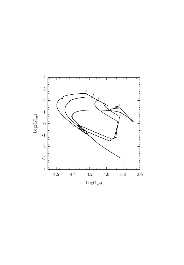
Figure 1: The evolutionary track for the primary component of system 1 ($M=2.0$ ${\rm M}_{\odot}$ , $q_{0}=1.5$, $P_{0}=1.5$ days). Dots labeled with odd (even) numbers indicate the onset (end) of mass transfer episodes. Notice that the star undergoes two hydrogen thermonuclear flashes each of them producing the large loops shown. For more details, see text.

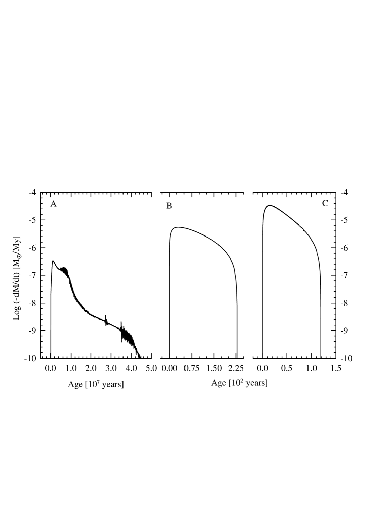
Figure 2: The mass transfer rate from the primary star of system 1. The star undergoes a long mass transfer episode soon after core hydrogen exhaustion (panel A). In panels B and C we depict the mass transfer rate corresponding to the episodes due to hydrogen thermonuclear flashes. Notice that they are, by far, shorter and with a maximum rate about two to three orders of magnitude larger than the corresponding to the first episode. In each panel, time is counted from the onset of mass transfer on. For the age of the star at these moments, see Table 1.

Here, $q_{0}\equiv M/M_{2}$ is the initial the mass ratio of the binary components and $P_{0}$ the initial orbital period. The evolutionary track for the primary component of system 1 is shown in Fig. 1 and the conditions at the beginning (points labelled with odd numbers) and end (points labelled with even numbers) of mass transfer episodes are included in Table 1. The star fills its Roche lobe soon after the end of core hydrogen burning. From then on, the star begins to transfer mass on a timescale of $\approx 10^{7}$ y (see Fig. 2). The star ends the first mass transfer episode with a much lower mass value (see Table 1) and begins to evolve bluewards to the white dwarf stage. This evolution is stopped, because the hydrogen envelope is still thick enough to ignite in a flash fashion, forcing the star to inflate on a very short timescale. Then, the star swells very suddenly and fills the corresponding Roche lobe again. Then, the star suffers from a second mass transfer episode depicted in the second panel of Fig. 2. In this second episode the total amount of mass transferred is very tiny and occurs on a very short timescale. As a consequence the Roche lobe size is almost constant and the star is forced to evolve along a constant - radius line. Now, after the end of the second mass transfer episode, the star has a thinner outer hydrogen layer and evolves again bluewards to the white dwarf stage but again it suffers from a second hydrogen thermonuclear flash. Then, the history is repeated: the star suddenly swells up and fills the Roche lobe by third time. Mass transfer begins and again a very little amount of mass is transferred but now in a much shorter timescale compared to the case of the immediately previous mass transfer episode. After ending this third mass transfer episode, the star evolved again bluewards to the white dwarf stage and cools down without suffering any other flash.

As it is well known, hydrogen thermonuclear flashes occur very near the stellar surface. As the hydrogen rich outer layer is very thin, if we want to compute all these stages properly, we do need to consider a very fine zoning for these critical layers. As previously mentioned, at flash - induced mass transfer episodes, a very tiny fraction of the star is lost before the star detaches and starts to evolve bluewards again. Then, we do also need a very thin zoning in order to account properly for the exact amount of hydrogen remaining in the star, as well as the large gravitational energy release when the star undergo large radius excursions. This is the kind of physical situation that suggested us the convenience of designing our binary evolution code in the way we have presented in the previous sections, especially regarding the treatment of the outer layers and the amount of matter we allow to be above the outermost finite - differenced zone.

We remark that, assuming this fully implicit scheme including the MTR we have found that the most difficult quantity to compute is just the MTR. This is especially true when the outer layers become in convective equilibrium. This is reflected in some strong oscillations shown in the first panel of Fig. 2. In any case we feel this not to affect the main course of the evolution. Remarkably, such oscillations are not present in the flash - induced mass transfer episodes.

System 2 is a Class A system (see Fig. 4) which transfers most of its mass when it is still burning hydrogen in the core. Then, it suffers three thermonuclear flashes with its corresponding mass transfer episodes in a way very similar to the corresponding to System 1 (see Table and Figs. 5 and 6).

System 3 (Class B) suffers from four mass transfer episodes, three of them induced by each thermonuclear flash. The main characteristics of these evolutionary calculations are included in Figs. 7 - 9 and in Tables 2 and 3 we include the conditions at the onset and end of mass transfer episodes.

System 3 evolution can be compared with the results presented by Podsiadlowski et al. (2001) in their Fig. 14. They evolved a system composed initially by a 1.4 $M_{\odot}$ normal star and a neutron star of the same mass. Mass transfer begins near the end of core hydrogen burning. In doing so, they employed a full nuclear reaction network, convective overshooting, and different assumptions about mass transfer from the ones we have done here. In particular, they used $\beta=0.5$, i.e., that half of the mass lost by the normal star is accreted by the neutron star as long as the rate is smaller than the Eddington limit ($\approx 10^{-8}M_{\odot}/y$). Also, they considered $\alpha=1$ for the angular momentum losses. Clearly, these are large differences compared with our System 3 and also with the physical ingredients we considered in the present paper. Notice that Podsiadlowski et al. (2001) found three hydrogen thermonuclear flashes, two of which leading to Roche lobe overflow. In our system, we also have three hydrogen flashes, all of them leading to lobe overflow. This is an important difference that we suspect it to be related with the different assumptions in the orbital evolution of the system. We also consider that the differences in the treatment of nuclear energy release are of key importance. Clearly, our equilibrium cycles predict stronger flashes. However, notice that the mass of the final helium white dwarf is very similar in both calculation (0.199 $M_{\odot}$ for Podsiadlowski et al. 2001).

Table 1: Selected evolutionary stages of system 1

Point	$Age/10^{9}y$	$M/M_{\odot}$	$Log(L/L_{\odot})$	$Log(T_{eff})$	$P\;[d]$
1	8.6344152	2.00000	1.470297	3.862974	1.500
2	9.0981136	0.23161	0.950006	3.833146	2.442
3	9.6587255	0.23161	2.026359	4.102230	2.442
4	9.6587278	0.23096	2.306213	4.171956	2.449
5	9.9650518	0.23096	1.740276	4.030472	2.449
6	9.9650530	0.22935	2.608005	4.246795	2.468

Table 2: Selected evolutionary stages of system 2

Point	$Age/10^{9}y$	$M/M_{\odot}$	$Log(L/L_{\odot})$	$Log(T_{eff})$	$P\;[d]$
1	0.42652401	2.00000	1.280174	3.925827	0.697
2	9.68186661	0.18421	0.179932	3.785182	1.006
3	10.1453763	0.18421	1.100802	4.015836	1.007
4	10.1453778	0.18395	1.163948	4.031070	1.008
5	10.1883408	0.18421	1.099444	4.015355	1.008
6	10.1883427	0.18348	1.341075	4.075097	1.011
7	10.2173678	0.18348	1.217356	4.044674	1.011
8	10.2173692	0.18313	1.417843	4.094100	1.013

Table 3: Selected evolutionary stages of system 3

Point	$Age/10^{9}y$	$M/M_{\odot}$	$Log(L/L_{\odot})$	$Log(T_{eff})$	$P\;[d]$
1	2.0641016	1.40000	0.844531	3.797418	1.000
2	3.4962904	0.20567	0.472654	3.702205	2.803
3	3.8905910	0.20567	1.053372	3.847385	2.803
4	3.8905929	0.20530	1.278767	3.903560	2.809
5	3.9239877	0.20530	1.299815	3.908821	2.809
6	3.9239887	0.20490	1.546744	3.970370	2.815
7	4.0033926	0.20490	1.385939	3.930169	2.815
8	4.0033931	0.20415	1.853513	4.046706	2.827

Finally, in Fig. 10 we show the evolution of the central part of the three computed objects in the temperature - density plane. As expected, the evolution is rather similar and is limited to temperatures below helium ignition. The flash episodes suffered by these objects are responsible for the oscillation in the temperature of the star before it gets near the final density value. Then, the objects cool down almost at constant central density, as it should be expected.

These calculations indicate that the above described scheme is capable of handling the evolution of close binary systems in a very adequate way. In our opinion, the here described code should be a valuable tool in handling binary evolution. Let us remark that, we have tested the code with low mass systems because are the ones we are most interested in. Also, we have found very good convergence of the method for the case of massive CBSs.

In closing, we should remark that the above described results should not be considered a state - of - the - art evolutionary calculations but a serious test of the numerical scheme as a previous step for future works. This is so mainly because of the lack of a detailed nuclear reactions network and also for the absence of a treatment of diffusion. Notice that diffusion is a key process in the evolution of objects in the range of masses we have here considered and even largely determine the total number of thermonuclear flashes the object suffers from (see Althaus, et al. 2001).

8 Discussion and Future Applications

In this paper we have presented a Henyey-type code tailored for computing stellar evolution in close binary systems (CBSs). This code is a modification of the scheme presented long ago by Kippenhahn, Weigert & Hofmeister (1967) for the case of the evolution of isolated objects.

Here we considered that mass transfer occurs when the star overflows its Roche lobe. The main characteristic of the present code is that it automatically computes the beginning and end of mass transfer stages, computing the MTR of the object in a fully implicit, self consistent fashion. Perhaps, main shortcoming of the scheme we have presented is that it is not able to compute common envelope evolution, simply because at these stages it is not possible to equate the radius of the star to that of the Roche lobe.

In the present version of the code, we have considered radiative OPAL and conductive opacities, neutrino emissivities, convection following the mixing length prescription, and a detailed equation of state. The nuclear reactions have been considered only by means of the equilibrium cycles. Regarding the physics of mass transfer, we have considered the possibility that a fraction of the mass transferred from the primary is accreted by the secondary. Also we have included angular momentum dissipation due to gravitational radiation and magnetic braking.

We have found that the scheme detailed above is able to handle most of the evolutionary stages suffered by a donor star belonging to a CBS. Apart from the results we have presented as a first application, we have also tested it for the case of massive CBSs finding it to be very adequate also for these purposes. Generally speaking, the code is able to perform single stellar evolution and also to find the onset and end of each mass transfer episode. In all the test calculations we have performed we found it much more easy to compute a mass transfer rates (MTRs) when outer layers are in radiative equilibrium. In the case of convective layers convergence is attained but sometimes it is necessary a larger number of iterations.

As a first application of this code to astrophysically relevant conditions, we have applied it to the case of the formation of low mass helium white dwarfs. These computations should not be considered as a state - of - the - art ones but as a test of the numerical scheme as a previous step for future works. This is so mainly because of the lack of a detailed nuclear reactions network and also for the absence of a treatment of diffusion.

We expect that the physical and numerical performance of the code should be largely improved if we replace the outer boundary condition for the stellar radius by the formulation of Ritter (1988) for mass loss transfer (see the Introduction). This should be especially important at the beginning and end of each mass transfer episode and/or in the case of very low mass transfer rates. Also, the implementation of a moving grid should help in producing smooth curves of mass loss vs. time.

As a future application for the present code we plan to study the problem of the formation of helium white dwarfs including the complete physical ingredients we have considered in the previous works of our group on this topic. Also, we plan to study the relevance of the irradiation (Tout, et al. 1989; D’Antona & Ergma 1993) in the evolution of the members of CBSs. This should be especialy relevant for the case of LMXBs which in some evolutionary stages are expected to undergo mass transfer driven by irradiation (Podsiadlowski 1991).

Fig. 4 - 10 are available upon request to the authors at their e-mail addresses.

9 Acknowledgements

The authors want to warmly acknowledge our referee Prof. Phillip Podsiadlowski for his very constructive criticism and advice. This has enabled us not only to improve the original version of this work significantly but also has helped us on how to upgrade the performance of the code we presented here from a physical and numerical point of view.

Also, OGB wants to acknowledge Prof. Francesca D’Antona for discussion about the problem of computing binary evolution.

Figure 3: The Orbital period and semiaxis as a function of the mass of the primary star of system 1.

References

- [1] Althaus, L. G., Serenelli, A. M., Benvenuto, O. G. 2001, ApJ, 554, 1110
- [2] Arnett, W. D., Truran, J. W. 1969, ApJ, 157, 339
- [3] Bhattacharya, D., van den Heuvel, E. P. J. 1991, Phys. Rep., 203, 1
- [4] Clayton, D. D., 1968, Principles of Stellar Evolution and Nucleosynthesis, J. Wiley
- [5] Eggleton, P. P. 1983, ApJ, 268, 368
- [6] D’Antona, F., Ergma, E. 1993, A&A, 269, 219
- [7] Han, Z., Tout, C. A., Eggleton, P. P. 2000, MNRAS, 319, 215
- [Iben(1985)] Iben, I. 1985, QJRAS, 26, 1
- [8] Iben, I., Livio, M. 1993, PASP, 105, 1373
- [9] Kippenhahn, R., Weigert, A. 1967, Zeitschrift Astrophysics, 65, 251
- [10] Kippenhahn, R., Kohl, K., Weigert, A. 1967, Zeitschrift Astrophysics, 66, 58
- [11] Kippenhahn, R., Thomas, H.-C., Weigert, A. 1968, Zeitschrift Astrophysics, 69, 265
- [12] Kippenhahn, R., Weigert, A. 1990, Stellar Structure and Evolution, Springer-Verlag
- [Kutter & Sparks(1972)] Kutter, G. S., Sparks, W. M. 1972, ApJ, 175, 407
- [13] Landau, L. D., Lifshitz, E. M. 1959, The Clasical Theory of Fields, Pergamon Press
- [14] Lauterborn, D. 1970, A&A, 7, 150
- [15] Paczyński, B. 1971, ARA&A, 9, 183
- [16] Podsiadlowski, P. 1991, Nat, 350, 654
- [17] Podsiadlowski, P., Joss, P. C., Hsu, J. J. L. 1992, ApJ, 391, 246
- [18] Podsiadlowski, P., Rappaport, S., Pfahl, E. D. 2002, ApJ, 565, 1107
- [19] Press, W. H., Teukolsky, S. A., Flannery, B. P., Vetterling, W. T. 1992, Numerical Recipes, Cambridge Univ. Press
- [20] Rappaport, S., Joss, P. C., Webbink, R. F. 1982, ApJ, 254, 616
- [21] Rappaport, S., Joss, P. C., Verbunt, F. 1983, ApJ, 275, 713
- [22] Ritter, H. 1988, A&A, 202, 93
- [23] Savonije, G. J. 1978, A&A, 62, 317
- [Taam & Sandquist(2000)] Taam, R. E., Sandquist, E. L. 2000, ARA&A, 38, 113
- [24] Tout, C. A., Eggleton, P. P., Fabian, A. C., Pringle, J. E. 1989, MNRAS, 238, 427
- [van der Klis(2000)] van der Klis, M. 2000, ARA&A, 38, 717
- [25] Verbunt, F., Zwaan, C. 1981, A&A, 100, L7
- [26] Wagenhuber, J., Weiss, A. 1994, A&A, 286, 121
- [27] Wellstein, S., Langer, N., Braun, H. 2001, A&A, 369, 939
- [28] Ziolkowski, J. 1970, AcA, 20, 59