A Microcalorimeter and Bolometer Model

Abstract

The standard non-equilibrium theory of noise in ideal bolometers and microcalorimeters fails to predict the performance of real devices due to additional effects that become important at low temperature. In this paper we extend the theory to include the most important of these effects, and find that the performance of microcalorimeters operating at 60 mK can be quantitatively predicted. We give a simple method for doing the necessary calculations, borrowing the block diagram formalism from electronic control theory.

Introduction

A complete non-equilibrium theory for the noise in simple bolometers with ideal resistive thermometers was given by J. C. Mather in 1982 mather82 and extended to microcalorimeter performance two years later moseley . Here we use the terms bolometer and calorimeter in the conventional sense, respectively indicating power detectors and integrating energy detectors.

This theory shows that the performance of these devices improves dramatically as the operating temperature is reduced. However, at temperatures below $\sim$200 mK, it becomes increasingly difficult to construct a bolometer that behaves according to the ideal assumptions. The resistance of the thermometer becomes dependent on readout power as well as temperature and equilibration times between different parts of the detector become significant. Thermodynamic fluctuations between internal parts are then an additional noise source. The physical description for most of these effects is straightforward, but combining all of them into a detector model can be algebraically daunting.

Theoretical models that describe complex thermal architectures are necessary to understand the behavior of real devices, and some groups have already extended the “ideal” model developed by J. C. Mather in 1982 to include some non-ideal effects in order to explain their experimental results hoevers ; gildemeister ; flei ; piat . We developed a general bolometer and microcalorimeter model using the block diagram formalism of control theory. The formalism helps with the mechanics of the problem, while keeping the physical model reasonably transparent lee ; nivelle ; max_feed . In the model we have included the thermal decoupling between the electron system and the phonon system in the thermometer, the so called hot-electron model, the thermal decoupling between the absorber and the thermometer, and non-ohmic behaviors of the thermometer in addition to the hot-electron effect. The hot-electron model assumes that the resistance of the thermometer depends on the temperature of the electrons, and there is a thermal resistance between the electrons and the crystal lattice through which the bias power must flow, increasing the temperature of the electrons above the temperature of the lattice, and therefore changing the thermometer resistance. This effect is well known in metals at low temperatures and has recently been studied in semiconductors in the variable range-hopping regime wang ; g_hot-el ; dahai . The noise analysis incorporates terms for thermometer Johnson and $1/f$ noise, amplifier noise, load resistor Johnson noise, and thermodynamic fluctuations between the electron and phonon systems in the thermometer as well as between the absorber, the thermometer, and the heat sink. In the model we also included the effect of thermometer non-ohmic behavior, i.e. dependence of the thermometer resistance on the bias signal. This effect is particularly important when Transition Edge Sensors (TES) are used mark and makes the model valuable for predicting the performance of this type of detector.

I The ideal model

To help the reader understand the algebra of our model we decided to start our analysis with an overview of the ideal model that has been previously developed. Despite their different applications, bolometers and microcalorimeters are very similar detectors and the theory of their operation is largely the same. The considerations of this paper apply to both kinds of detectors unless otherwise specified and we will use the generic term “detectors” to refer to both.

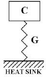
Figure 1: Thermal sketch of a bolometer or microcalorimeter

Typically a bolometer or a microcalorimeter is composed of three parts: an absorber that converts the incident power or energy into a temperature variation, a sensor that reads out the temperature variation, and a thermal link between the detector and a heat sink. The sensor is typically a resistor whose resistance strongly depends on the temperature around the working point. An ideal detector can be represented by a discrete absorber of heat capacity $C$ in contact with the heat sink through a thermal conductivity $G$ (see Fig. 1), and a thermometer always at the temperature of the absorber. The thermometer sensitivity is specified by:

$$\alpha\equiv\frac{T}{R}\frac{dR}{dT},$$ (1)

where $T$ is the detector temperature and $R$ is the sensor resistance. The thermal conductivity $G$ is defined as:

$$G\equiv\frac{dP}{dT},$$ (2)

where $P$ is the power dissipated into the detector. The conductivity $G$ can generally be expressed as a power law of the detector temperature $T$, i.e. $G=G_{0}\cdot T^{\beta}$. Notice that numerically $G_{0}$ is equal to the thermal conductivity at 1 K, but dimensionally $G_{0}$ is a thermal conductivity divided by a temperature to the $\beta$.

In equilibrium, with no other input power than the Joule power $P$ used to read out the thermometer resistance, the equilibrium temperature of the detector $T$ is determined by integrating Eq. 2 between the heat sink temperature $T_{S}$ and the detector temperature:

$$\int_{T_{S}}^{T}G(T^{\prime})dT^{\prime}=P(T).$$ (3)

Assuming the power law expression for $G$ introduced before and integrating it becomes:

$$(T^{\beta+1}-T_{S}^{\beta+1})=\frac{\beta+1}{G_{0}}P(T).$$ (4)

It is important to remember, when calculating the equilibrium temperature, that the power $P$ depends on the value of the sensor resistance and, as a consequence, it depends on the temperature $T$, as explicitly indicated in Eq. 4. To calculate the equilibrium temperature it is therefore necessary to solve the system of equations represented by Eq. 4, the $P$ vs. $R$ curve and the $R$ vs. $T$ curve. In general,the system must be solved numerically.

Of interest from the point of view of the detector operation, is how the temperature rise $\Delta T$ above the equilibrium temperature depends on an external incident power $W$. The power input to the detector ($W+P$) is partly stored into the heat capacity of the detector and partly flows to the heat sink through the thermal conductivity. The equation that determines the generic temperature $T_{D}$ of the detector is therefore:

$$C\frac{dT_{D}}{dt}+\int_{T_{S}}^{T_{D}}G(T^{\prime})dT^{\prime}=W+P(T_{D}),$$ (5)

where we explicitly indicated that the bias power can be a function of the temperature $T_{D}$ and where the quantities $T_{D}$, $W$, and $P$ can be a function of time $t$. We can express the generic detector temperature $T_{D}$ as a function of the equilibrium temperature $T$ defined in Eq. 4 as $T_{D}=T+\Delta T$. Eq. 5 then becomes:

$$C\frac{d(T+\Delta T)}{dt}+\int_{T_{S}}^{T}G(T^{\prime})dT^{\prime}+\int_{T}^{T+\Delta T}G(T^{\prime})dT^{\prime}=W+P(T+\Delta T).$$ (6)

If we stay in the so called small signal limit, i.e. we assume that $\Delta T$ is small compared to $T$, we can expand the second integral to lowest order in $\Delta T/T$, obtaining:

$$C\frac{d(T+\Delta T)}{dt}+\int_{T_{S}}^{T}G(T^{\prime})dT^{\prime}+G(T)\cdot\Delta T=W+P(T)+\Delta P$$ (7)

with $\Delta P=P(T+\Delta T)-P(T)$. Subtracting Eq. 3 from Eq. 7, and considering that the equilibrium temperature $T$ does not change with time, we obtain:

$$C\frac{d(\Delta T)}{dt}+G\cdot\Delta T=W+\Delta P,$$ (8)

where for simplicity we expressed $G\equiv G(T)$.

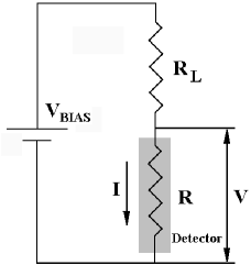
Figure 2: Typical detector readout circuit.

In general, the bias power will change with temperature, since $R$ changes, and its expression depends on the bias source impedance. A typical bias circuit is illustrated in Fig. 2 where $R$ is the thermometer resistance and $R_{L}$ is a load resistor. The most commonly used bias conditions are near current bias ($R_{L}\gg R$) and near voltage bias ($R_{L}\ll R$). More complex bias circuits are also used, and can always be represented by the circuit of Fig. 2 using Thevenin equivalence theorems. Differentiating the expression for the Joule power $P=I^{2}R=V^{2}/R$ and using the bias circuit of Fig. 2 we obtain:

$$\Delta P=-\frac{P}{T}\frac{R-R_{L}}{R_{L}+R}\alpha\Delta T.$$ (9)

This term is generally referred to as the electro-thermal feedback term and it often plays an important role in the response of a detector. For simplicity in the small signal analytical calculations, we write the electro-thermal feedback term as:

$$\Delta P=-G_{\mathit{ETF}}\Delta T,$$ (10)

where

$$G_{\mathit{ETF}}\equiv\frac{P}{T}\frac{R-R_{L}}{R_{L}+R}\alpha,$$ (11)

so that Eq. 8 becomes:

$$C\frac{d(\Delta T)}{dt}+(G+G_{\mathit{ETF}})\cdot\Delta T=W$$ (12)

or, introducing an equivalent thermal conductivity $G_{\mathit{eff}}=G+G_{\mathit{ETF}}$ (which we refer to as effective thermal conductivity):

$$C\frac{d(\Delta T)}{dt}+G_{\mathit{eff}}\cdot\Delta T=W.$$ (13)

The easiest way to solve this differential equation is using Fourier transforms. The procedure is to use Fourier transforms to convert the terms of Eq. 13 to the frequency domain, solve the equation in the frequency domain where it becomes a linear equation, then Fourier invert transform the result to the time domain. The advantage of solving Eq. 13 in the frequency domain comes from the fact that the expression $d\Delta T(t)/dt$ in the frequency domain becomes $j\omega\Delta T(\omega)$, where we used the engineering notation $j=\sqrt{-1}$. Equation 13 in the frequency domain then becomes:

$$j\omega C\Delta T(\omega)+G_{\mathit{eff}}\cdot\Delta T(\omega)=W(\omega).$$ (14)

whose solution is:

$$\Delta T(\omega)=\frac{1}{G_{\mathit{eff}}}\frac{1}{1+j\omega\tau_{\mathit{eff}}}W(\omega)$$ (15)

with $\tau_{\mathit{eff}}=C/G_{\mathit{eff}}$.

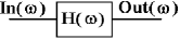
Figure 3: Block diagram representation of a system with transfer function $H(\omega)$.

The detector system behaves as a low pass system, with time constant $\tau_{\mathit{eff}}$. For negative electrothermal feedback $G_{\mathit{ETF}}$ must be positive and the detector time constant is shortened. For positive feedback $G_{\mathit{ETF}}$ is negative and the detector time constant is lengthened and, in the case of $|G_{\mathit{ETF}}|$ bigger than $G$, the detector becomes unstable. The sign of $G_{\mathit{ETF}}$ depends on the sign of $\alpha$ and on the bias condition used (i.e., the ratio $R/R_{L}$). In the small-signal (linear) limit considered here and in absence of amplifier noise, the signal has no effect on the detector performance. However positive feedback reduces the effect of amplifier noise, while negative feedback helps linearize the large signal gain, and improves microcalorimeter resolution for large signals at high count rate. Since it can usually be arranged that amplifier noise is negligible, these practical considerations normally favor negative feedback. People then use current bias ($R<R_{L}$) for detectors with negative $\alpha$ and voltage bias ($R>R_{L}$) for detectors with positive $\alpha$.

In operating a detector, what is really detected is not directly the temperature variation $\Delta T$, but the resistance variation $\Delta R$, which is read out either as a voltage or current variation, that is:

$$\Delta V=V\frac{\alpha}{T}\frac{R_{L}}{R_{L}+R}\Delta T$$ (16)

$$\Delta I=-I\frac{\alpha}{T}\frac{R}{R_{L}+R}\Delta T.$$ (17)

We can generically indicate the output signal as $X$ and the relation between the output and the temperature as:

$$\frac{\Delta X}{X}=\alpha\cdot A_{tr}\frac{\Delta T}{T}$$ (18)

where $A_{tr}$ is a dimensionless parameter that quantifies how much the output signal is sensitive to resistance changes and that we call the transducer sensitivity. Numerically $A_{tr}$ is defined as:

$$A_{tr}\equiv\frac{R}{X}\frac{dX}{dR}.$$ (19)

Notice that the expression of $A_{tr}$ can be easily derived from Eqs. 18 and 16 or 17 for voltage and current readout, and is always smaller or equal to unity for passive bias circuit ($R_{L}>0$).

The response of a detector is usually quantified by the responsivity $S(\omega)$, defined as:

$$S(\omega)=\frac{\Delta X(\omega)}{W(\omega)}$$ (20)

that is, the responsivity characterizes the response of the detector, $\Delta X$, to an input power $W$. In the ideal model just described we can combine Eqs. 15 and 18 to obtain:

$$\Delta X(\omega)=\frac{1}{G_{\mathit{eff}}}\frac{1}{1+j\omega\tau_{\mathit{eff}}}\frac{X\cdot\alpha\cdot A_{tr}}{T}\cdot W(\omega),$$ (21)

and the responsivity is then equal to:

$$S(\omega)=\frac{1}{G_{\mathit{eff}}}\frac{1}{1+j\omega\tau_{\mathit{eff}}}\frac{X\cdot\alpha\cdot A_{tr}}{T}.$$ (22)

A detector at the working point is also often described by the complex dynamic impedance $Z(\omega)=dV(\omega)/dI(\omega)$. The dynamic impedance $Z(\omega)$ differs from the detector resistance $R=V/I$ due to effect of the electro-thermal feedback. When the current changes, the power dissipated into the detector changes too, therefore the temperature and the detector resistance change. It is often useful to express the detector performance and characteristics in terms of the dynamic impedance since it can be easily measured experimentally.

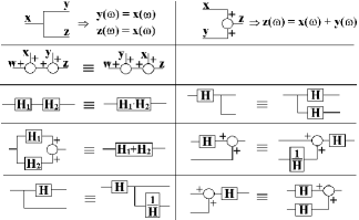
Figure 4: Some general operations with the block diagram algebra.

The calculation of the analytical expression of the dynamic impedance is simple. Differentiating Ohm’s law, $V=I\cdot R$, we obtain:

$$dV=I\cdot dR+R\cdot dI.$$ (23)

Using Eq. 8 in the frequency domain with $W=0$ and the definition of the thermometer sensitivity $\alpha$ in Eq. 1, we obtain:

$$dR=\frac{R}{T}\alpha dT=\frac{R\alpha}{GT}\frac{1}{1+j\omega\tau}dP.$$ (24)

with $\tau=C/G$. This $\tau$ is called the “intrinsic” or “thermal” time constant of the detector. Differentiating the expression of the Joule power dissipated into the thermometer $P=V\cdot I$, we obtain:

$$dP=V\cdot dI+I\cdot dV,$$ (25)

which, combined with Eqs. 23 and 24 gives:

$$dV=R\cdot dI+I\frac{R\alpha}{GT}\frac{1}{1+j\omega\tau}(I\cdot dV+V\cdot dI).$$ (26)

Notice that in Eqs. 23 through 26 most of the terms are function of the frequency $\omega$. Solving Eq. 26 we obtain:

$$Z(\omega)=\frac{dV(\omega)}{dI(\omega)}=R\frac{1+\frac{P\alpha}{GT}+j\omega\tau}{1-\frac{P\alpha}{GT}+j\omega\tau}=Z_{0}\frac{1+j\omega\tau\frac{Z_{0}+R}{2Z_{0}}}{1+j\omega\tau\frac{Z_{0}+R}{2R}},$$ (27)

where we used the expression

$$Z_{0}=Z(\omega=0)=R\frac{1+\frac{P\alpha}{GT}}{1-\frac{P\alpha}{GT}}.$$ (28)

Notice that when $\omega\rightarrow\infty$, $Z\rightarrow R$.

The dynamic impedance, $Z(\omega)=dV/dI$, is easily measured experimentally. It can be determined most readily by adding a small A.C. signal to the bias voltage and measuring the transfer function of the detector $TF(\omega)$. This is the ratio of amplitudes and relative phase between changes in the detector voltage and changes in the bias voltage as a function of frequency. Most spectrum analyzers have the capability of measuring the complex ratio between two signals as a function of frequency, and can do this simultaneously over the frequency range of interest using a band-limited white noise source. Signal averaging allows very precise measurement to be made while remaining in the small-signal limit. The dynamic impedance is easily derived from the transfer function using the value of the load resistance and making appropriate corrections for stray electrical capacitance or inductance in the circuit. For example, in the bias circuit of Fig. 2, without stray capacitance, the impedance is equal to: $Z(\omega)=R_{L}\cdot TF(\omega)/(1-TF(\omega))$.

It is then possible to determine values for many of the important parameters of the detector by fitting the real and imaginary parts of the transfer function by adjusting the thermal and electrical parameters in the expressions given in this paper. This is very valuable for diagnosing performance problems or improving the design of detectors. Note that when the thermometer temperature coefficient $\alpha$ is positive, the impedance can become infinite. It is then more convenient to work with the inverse quantity $1/Z(\omega)=dI/dV$.

In the case of a detector whose signal is read out as a voltage change, where the responsivity $S$ is defined as $S(\omega)=dV(\omega)/dW(\omega)$, we can also write:

$$S(\omega)=\frac{1}{2I}\frac{(Z_{0}/R)-1}{(Z_{0}/R_{L})+1}\frac{1}{1+j\omega\tau_{\mathit{eff}}}.$$ (29)

At this point we want to introduce a useful technique for analyzing the response of a bolometer or a microcalorimeter: block diagram algebra. This technique is generally used in electrical engineering to analyze feedback systems and it is very useful when extending the theory of bolometers and microcalorimeters to more complicated realistic systems. The algebra of block diagrams and the language of control theory have been successfully used before in the analysis of microcalorimeters and bolometer lee ; nivelle ; max_feed . The basic idea is that a system with transfer function in the frequency domain equal to $H(\omega)$ is represented by the diagram of Fig. 3. If an input $In(\omega)$ is applied to the system the output is $Out(\omega)=H(\omega)\cdot In(\omega)$. Complicated systems can always be reduced to the system of Fig. 3 using the block diagram algebra. Fig. 4 shows some of the common operations that will be used in this paper. The procedure to solve the response of a system using the block diagram algebra is then the following:

• Write the differential equations that define the system response.

• Convert the equations to the frequency domain and, for each equation define the individual system response and the input to that system.

• Layout the block diagram that describes all the equations together.

• Use the block diagram algebra to reduce the block diagram to the form of Fig. 3 that represents the system response in the frequency domain.

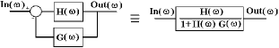
Figure 5: Block diagram representation of a feedback system.

This representation is particularly useful to deal with feedback systems, i.e. systems where the output is combined to the input through a transfer function $G(\omega)$ as in Fig. 5. In this case, whenever an external input $In(\omega)$ is applied to the system the output is:

$$Out(\omega)=\frac{H(\omega)}{1+H(\omega)G(\omega)}In(\omega)=H_{\mathit{c-l}}(\omega)\cdot In(\omega),$$ (30)

where $H_{\mathit{c-l}}(\omega)$ is called the closed loop transfer function.

Going back to the theory of bolometers and microcalorimeters, we can write Eq. 12 as:

$$C\frac{d(\Delta T)}{dt}+G\cdot\Delta T=W-G_{\mathit{ETF}}\cdot\Delta T,$$ (31)

that, in the frequency domain, becomes:

$$j\omega C\Delta T+G\Delta T=W-G_{\mathit{ETF}}\Delta T.$$ (32)

We now want to generate the block diagram describing this equation. The left part represents the response of the system that we are analyzing (the output $\Delta T$ as a function of an input power), while the right part represents the input to that system. The fact that the input depends on the output $\Delta T$ is a consequence of feedback. The left part of the equation represents a low pass system with transfer function

$$H(\omega)=\frac{1}{G}\frac{1}{1+j\omega\tau}$$ (33)

The input consists of an external input $W$ minus the output itself modified by the transfer function $G_{\mathit{ETF}}$. This is a typical feedback system represented by the block diagram of Fig. 6, where we also included the conversion of $\Delta T$ to $\Delta X$. If we now solve the block diagram using the block diagram algebra and Eq. 30, we obtain:

$$\Delta X(\omega)=\frac{1}{G+G_{\mathit{ETF}}}\frac{1}{1+j\omega\frac{C}{G+G_{\mathit{ETF}}}}\frac{X\cdot\alpha\cdot A_{tr}}{T}W(\omega)=\frac{1}{G_{\mathit{eff}}}\frac{1}{1+j\omega\tau_{\mathit{eff}}}\frac{X\cdot\alpha\cdot A_{tr}}{T}W(\omega)$$ (34)

that is the same expression of Eq. 21.

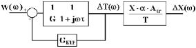
Figure 6: Block diagram representation of a detector.

II The Hot-electron Model

A first order correction to the standard theory of bolometers and microcalorimeters is the introduction of the hot-electron model. The model assumes that the thermal coupling between electrons and lattice in the sensor at low temperature is weaker than the coupling between electrons, so that the electric power applied to the electrons rises them to a higher temperature than the lattice. This behavior is a known property of metals and has recently been quantified in doped silicon dahai , so that it affects both TES and semiconductor sensors. The detector can therefore be described as composed of two different systems: the electron system and the phonon or lattice system and the two are thermally connected by a thermal conductivity $G_{\mathit{e-l}}$. We assume for models derived in this paper that the detector resistance responds to the temperature of its electron system, and that the Joule power of the bias is dissipated there. For economy of presentation, the models derived here assume the input power enters through the absorber phonon system, which is then thermally connected to the thermometer lattice, and further to the heat sink through the thermal conductivity $G$ (see Fig. 7). There are important classes of detectors where signal power is absorbed directly in the electron system of the thermometer or absorber, and the primary thermal path to the heat sink could be from the absorber lattice or either electron system. In the general case, these all result in different thermal circuits, and the block diagrams must be modified accordingly. In the approximation of this section, the phonon system includes both the absorber and the phonons in the thermometer (we will discuss later the case of a decoupled absorber).

In equilibrium with no external power, the electron system is at a higher temperature than the phonon system is and the Joule power flows from the electron system to the phonon system and from there to the heat sink. The equilibrium temperature of the two systems without any signal power applied can be calculated in a way similar to that used for the simple model described in the previous paragraph. As reported in the literature, the thermal conductivity between electrons and phonons can be described as a power law of the electron temperature $T_{e}$ wang ; g_hot-el :

$$G_{\mathit{e-l}}=G_{0e}\cdot T_{e}^{\beta_{e}}.$$ (35)

From the definition of thermal conductivity, we also have:

$$G_{\mathit{e-l}}=\frac{dP}{dT_{e}}$$ (36)

and if we combine the two and integrate from the lattice temperature $T_{l}$ to the equilibrium electron temperature $T_{e}$ we obtain

$$T_{e}^{\beta_{e}+1}=\frac{\beta_{e}+1}{G_{0e}}\cdot P(T_{e})+T_{l}^{\beta_{e}+1}$$ (37)

where we explicitly indicated the dependence of the power $P$ on the electron temperature $T_{e}$. The equilibrium temperature of the lattice system is still determined by Eq. 4 that, in this case, can be written as:

$$(T_{l}^{\beta+1}-T_{S}^{\beta+1})=\frac{\beta+1}{G_{0}}P(T_{e}).$$ (38)

Equations 37 and 38 represent a system with two variables $T_{e}$ and $T_{l}$ that can be solved numerically.

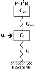
Figure 7: Thermal sketch of a bolometer or microcalorimeter in the hot electron model

Here we are considering detectors where the external power is absorbed in the phonon system, and the sensitivity of the detector can be strongly affected by the reduced sensitivity of $T_{e}$ to changes in $T_{l}$ introduced by the equilibrium difference of these temperatures and non-linear nature of $G_{\mathit{e-l}}$. We consider these effects in two steps. A first approximation is to assume that the heat capacity of the electron system is negligible. This case can be solved easily, and it is sufficient in many cases. We will then derive the general result for $C_{e}\neq 0$.

II.1 Hot Electron Model with $C_{e}$ = 0

If the electron system heat capacity $C_{e}$ can be neglected, the dependence of the electron temperature on the lattice temperature is simply determined by Eq. 37. When the temperature of the lattice system changes by ${\Delta T_{l}}$ the temperature of the electron system will instantly change by $\Delta T_{e}$ and Eq. 37 becomes:

$$(T_{e}+\Delta T_{e})^{\beta_{e}+1}=\frac{\beta_{e}+1}{G_{0e}}\cdot P(T_{e}+\Delta T_{e})+(T_{l}+\Delta T_{l})^{\beta_{e}+1}.$$ (39)

If we subtract Eq. 37 from Eq. 39 we obtain

$$(T_{e}+\Delta T_{e})^{\beta_{e}+1}-T_{e}^{\beta_{e}+1}=\frac{\beta_{e}+1}{G_{0e}}(P(T_{e}+\Delta T_{e})-P(T_{e}))+(T_{l}+\Delta T_{l})^{\beta_{e}+1}-T_{l}^{\beta_{e}+1}.$$ (40)

Assuming that $\Delta T_{e}\ll T_{e}$ and $\Delta T_{l}\ll T_{l}$ we can expand Eq. 40 to lowest order in $\Delta T_{e}/T_{e}$ and $\Delta T_{l}/T_{l}$, obtaining:

$$(1+(\beta_{e}+1)\frac{\Delta T_{e}}{T_{e}})\cdot T_{e}^{\beta_{e}+1}-T_{e}^{\beta_{e}+1}=\frac{\beta_{e}+1}{G_{0e}}\cdot\Delta P+(1+(\beta_{e}+1)\frac{\Delta T_{l}}{T_{l}})\cdot T_{l}^{\beta_{e}+1}-T_{l}^{\beta_{e}+1}$$ (41)

that reduces to:

$$T_{e}^{\beta_{e}}\cdot\Delta T_{e}=\frac{\Delta P}{G_{0e}}+T_{l}^{\beta_{e}}\cdot\Delta T_{l}.$$ (42)

We already calculated the change in Joule power $\Delta P$ in Eqs. 9 and 10, that in the hot electron case depends on the change in electron temperature $\Delta T_{e}$:

$$\Delta P=-G_{\mathit{ETF}}\Delta T_{e},$$ (43)

therefore

$$\Delta T_{e}=\frac{T_{l}^{\beta_{e}}}{T_{e}^{\beta_{e}}+\frac{G_{\mathit{ETF}}}{G_{0e}}}\Delta T_{l}=\frac{G_{\mathit{e-l}}(T_{l})}{G_{\mathit{e-l}}(T_{e})+G_{\mathit{ETF}}}\Delta T_{l}=\frac{G_{\mathit{e-l}}(T_{l})}{G_{\mathit{e-l}}(T_{e})}\frac{1}{1+\frac{G_{\mathit{ETF}}}{G_{\mathit{e-l}}(T_{e})}}\Delta T_{l}=A_{\mathit{e-l}}\Delta T_{l}$$ (44)

where $G_{\mathit{e-l}}(T_{e})$ is the electron-lattice thermal conductivity calculated at the electron temperature and $G_{\mathit{e-l}}(T_{l})$ is the electron-lattice thermal conductivity calculated at the lattice temperature, and:

$$A_{\mathit{e-l}}=\frac{\Delta T_{e}}{\Delta T_{l}}=\frac{G_{\mathit{e-l}}(T_{l})}{G_{\mathit{e-l}}(T_{e})}\frac{1}{1+\frac{G_{\mathit{ETF}}}{G_{\mathit{e-l}}(T_{e})}}.$$ (45)

The quantity $A_{\mathit{e-l}}$ is adimensional and represents the temperature sensitivity of the thermometer. When $A_{\mathit{e-l}}=1$, the thermometer is completely sensitive to temperature changes in the lattice system, when $A_{\mathit{e-l}}=0$ the thermometer is completely insensitive to temperature changes in the lattice.

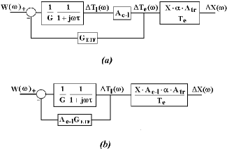
Figure 8: Block diagram representation of a detector using the hot electron model with $C_{e}=0$. (a) Block diagram as derived from the the equations that describe the detector. Notice that the representation of the $ETF$ as acting on the lattice system of the sensor is due to the fact that we are assuming that $C_{e}=0$. In general, if $C_{e}\neq 0$, the $ETF$ is an electric effect and acts on the electron system. (b) Equivalent representation to highlight the effect of the term $A_{e-l}$.

We now want to represent the detector using the block diagram algebra. The detector behavior is described by Eqs. 18, 31, and 44, that in the frequency domain can be written as:

$$j\omega C\Delta T_{l}+G\Delta T_{l}=W-G_{\mathit{ETF}}\Delta T_{e},$$ (46)

$$\Delta T_{e}=A_{e-l}\Delta T_{l},$$ (47)

and

$$\Delta X=\frac{X\alpha A_{tr}}{T_{e}}\Delta T_{e}.$$ (48)

Converting these three equations in block diagram algebra and connecting the blocks of the algebra together we obtain the representation of Fig. 8a. With some simple algebra, the diagram is equivalent to that of Fig. 8b, and considering that $G_{\mathit{ETF}}\propto\alpha$, the hot electron model with negligible heat capacity of the electron system is then equivalent to the standard model with the substitutions:

$$\alpha\rightarrow\alpha_{\mathit{eff}}=A_{\mathit{e-l}}\cdot\alpha$$ (49)

$$T\rightarrow T_{e}$$ (50)

and therefore the responsivity of the detector becomes

$$S(\omega)=\frac{1}{(G+A_{\mathit{e-l}}G_{\mathit{ETF}})}\frac{1}{(1+j\omega\tau_{\mathit{eff}})}\frac{A_{\mathit{e-l}}\cdot\alpha\cdot X\cdot A_{tr}}{T_{e}}.$$ (51)

with $\tau_{\mathit{eff}}=C_{l}/(G+A_{\mathit{e-l}}G_{\mathit{ETF}})$, where $C_{l}$ is the lattice heat capacity.

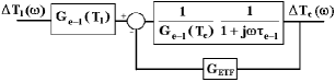
Figure 9: Representation of the electron system in the hot electron model with $C_{e}\neq 0$.

II.2 Hot Electron Model with C_e $\neq$ 0

If the heat capacity of the electron system is not negligible, the electron temperature is defined (in analogy to Eq. 5) by:

$$C_{e}\frac{dT_{e}}{dt}+\int_{T_{l}}^{T_{e}}G_{\mathit{e-l}}(T^{\prime})dT^{\prime}=P(T_{e})$$ (52)

with $G_{\mathit{e-l}}$ defined by Eq. 35. What we are interested in is the rise of the electron temperature $\Delta T_{e}$ above equilibrium when the lattice temperature rises by $\Delta T_{l}$. Eq. 52 then becomes

$$C_{e}\frac{d(T_{e}+\Delta T_{e})}{dt}+\int_{T_{l}+\Delta T_{l}}^{T_{e}+\Delta T_{e}}G_{\mathit{e-l}}(T^{\prime})dT^{\prime}=P(T_{e}+\Delta T_{e}).$$ (53)

Subtracting Eq. 52 from Eq. 53 we obtain

$$C_{e}\frac{d(\Delta T_{e})}{dt}+\int_{T_{e}}^{T_{e}+\Delta T_{e}}G_{\mathit{e-l}}(T^{\prime})dT^{\prime}-\int_{T_{l}}^{T_{l}+\Delta T_{l}}G_{\mathit{e-l}}(T^{\prime})dT^{\prime}=\Delta P$$ (54)

which, using Eq. 35 and expanding the result to lowest order in $\Delta T_{e}/T_{e}$ and $\Delta T_{l}/T_{l}$, becomes

$$C_{e}\frac{d(\Delta T_{e})}{dt}+G_{\mathit{e-l}}(T_{e})\Delta T_{e}=G_{\mathit{e-l}}(T_{l})\Delta T_{l}-G_{\mathit{ETF}}\Delta T_{e},$$ (55)

with $G_{\mathit{ETF}}$ defined by Eq. 43. The system of Eq. 55 is represented by the block diagram of Fig. 9 with $\tau_{\mathit{e-l}}=C_{e}/G_{\mathit{e-l}}(T_{e})$, which has the solution

$$\Delta T_{e}(\omega)=A_{\mathit{e-l}}\frac{1}{1+j\omega\tau_{e}}\Delta T_{l},$$ (56)

with $\tau_{e}=C_{e}/(G_{\mathit{e-l}}(T_{e})+G_{\mathit{ETF}})$ and $A_{\mathit{e-l}}$ defined by Eq. 45. Notice that Eq. 56 reduces to Eq. 44 if $C_{e}=0$.

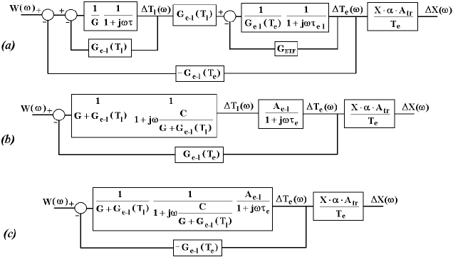
Figure 10: Block diagram representation of a detector using the hot electron model with $C_{e}\neq 0$. (a) Block diagram as derived from the equations describing the system. (b),(c) Intermediate steps for the solution of the block diagram representation.

The behavior of the lattice system is still regulated by Eqs. 5, 7 and 8, with the substitutions of $C_{l}$ for $C$ and of $T_{l}$ for $T$, i.e.:

$$C_{l}\frac{d(\Delta T_{l})}{dt}+G\cdot\Delta T_{l}=W+\Delta P_{l}.$$ (57)

The power $P_{l}$ is the power flowing from the electron system to the lattice system through the thermal conductivity $G_{\mathit{e-l}}$:

$$P_{l}=\int_{T_{l}}^{T_{e}}G_{\mathit{e-l}}(T^{\prime})dT^{\prime}.$$ (58)

Therefore

$$\Delta P_{l}=\int_{T_{e}}^{T_{e}+\Delta T_{e}}G_{\mathit{e-l}}(T^{\prime})dT^{\prime}-\int_{T_{l}}^{T_{l}+\Delta T_{l}}G_{\mathit{e-l}}(T^{\prime})dT^{\prime},$$ (59)

which, considering the expression of Eq. 35 for the thermal conductivity and expanding the result to lowest order in $\Delta T_{e}/T_{e}$ and $\Delta T_{l}/T_{l}$, becomes:

$$\Delta P_{l}=G_{\mathit{e-l}}(T_{e})\Delta T_{e}-G_{\mathit{e-l}}(T_{l})\Delta T_{l}.$$ (60)

Eq. 57 then becomes:

$$C_{l}\frac{d(\Delta T_{l})}{dt}+G\cdot\Delta T_{l}=W+G_{\mathit{e-l}}(T_{e})\Delta T_{e}-G_{\mathit{e-l}}(T_{l})\Delta T_{l}.$$ (61)

Equations 55 and 61 can be written in the frequency domain as:

$$j\omega C_{e}\Delta T_{e}+G_{\mathit{e-l}}(T_{e})\Delta T_{e}=G_{\mathit{e-l}}(T_{l})\Delta T_{l}-G_{\mathit{ETF}}\Delta T_{e}$$ (62)

and

$$j\omega C_{l}\Delta T_{l}+G\cdot\Delta T_{l}=W+G_{\mathit{e-l}}(T_{e})\Delta T_{e}-G_{\mathit{e-l}}(T_{l})\Delta T_{l},$$ (63)

and are represented by the block diagram of Fig. 10a. The diagram can be solved to obtain an analytical expression for the detector responsivity. In Figs. 10b and 10c we show two intermediate steps in the solution of the block diagram algebra. The detector responsivity is then equal to:

$$S(\omega)=\frac{1}{G_{\mathit{ETF}}A_{\mathit{e-l}}(1+j\omega\frac{C_{e}}{G_{\mathit{ETF}}})+G(1+j\omega\tau_{l})(1+j\omega\tau_{e})}\frac{A_{\mathit{e-l}}\cdot X\cdot\alpha\cdot A_{tr}}{T_{e}}.$$ (64)

with $\tau_{l}=C_{l}/G$. Notice that in the case of $C_{e}=0$ this expression reduces to Eq. 51, i.e. the hot electron model with negligible electron heat capacity, as expected.

Moreover, in the case of $G_{0e}\rightarrow\infty$, i.e. electrons and phonons can be thermally considered as a single system the responsivity becomes:

$$S(\omega)=\frac{1}{(G+G_{\mathit{ETF}})}\frac{1}{\left(1+j\omega\frac{C_{l}+C_{e}}{G+G_{\mathit{ETF}}}\right)}\frac{X\cdot A_{tr}\cdot\alpha}{T_{e}}.$$ (65)

This is just the ideal responsivity of a bolometer or microcalorimeter with thermal conductivity $G$, temperature $T_{e}$ and heat capacity $C=C_{l}+C_{e}$.

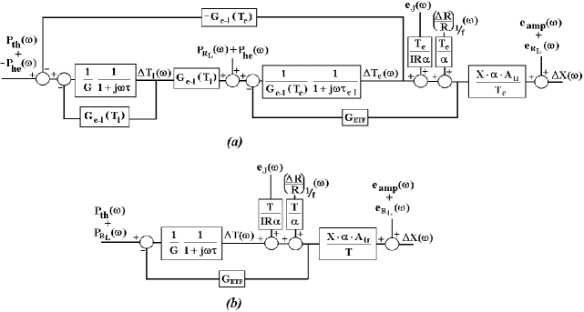
Figure 11: Block diagram representation of the noise in a a detector using the hot electron model(a) and equivalent representation for the ideal model (b). Notice that if the output $X$ is a current, the load resistor noise that adds to the output is represented by $i_{R_{L}}$.

In analogy to Eqs. 23 through 27, we can also calculate the dynamic impedance of the detector. We can write Eqs. 62 and 63 without external power $W$ and explicitly using the symbol $\Delta P$ for the change in Joule power: Converting Eqs. 55 and 61 to the frequency domain we obtain:

$$j\omega C_{e}\Delta T_{e}+G_{\mathit{e-l}}(T_{e})\Delta T_{e}=G_{\mathit{e-l}}(T_{l})\Delta T_{l}+\Delta P$$ (66)

and

$$j\omega C_{l}\Delta T_{l}+G\Delta T_{l}=G_{\mathit{e-l}}(T_{e})\Delta T_{e}-G_{\mathit{e-l}}(T_{l})\Delta T_{l}.$$ (67)

Combining Eqs. 1, 23, 25, 66 and 67, we then obtain:

$$Z(\omega)=R\frac{(G+G_{\mathit{e-l}}(T_{l})+j\omega C_{l})\left(G_{\mathit{e-l}}(T_{e})+j\omega C_{e}+\frac{P\alpha}{T_{e}}\right)-G_{\mathit{e-l}}(T_{e})\cdot G_{\mathit{e-l}}(T_{l})}{(G+G_{\mathit{e-l}}(T_{l})+j\omega C_{l})\left(G_{\mathit{e-l}}(T_{e})+j\omega C_{e}-\frac{P\alpha}{T_{e}}\right)-G_{\mathit{e-l}}(T_{e})\cdot G_{\mathit{e-l}}(T_{l})}$$ (68)

III Noise sources

There are several noise sources that affect the performance of bolometers and microcalorimeters, most of which have already been taken into account by Mather in 1982 mather82 . These include the Johnson noise of the sensor, the thermal noise due to the thermal link between the detector and the heat sink (also referred to as phonon noise), the Johnson noise of the load resistor used in the bias circuit and the noise of the read-out electronics (amplifier noise). In his paper Mather also mentions a $1/f$ noise contribution that seems to be more related to the sensor characteristics. This noise has been studied and quantified for silicon implanted thermistors by Han et al. in 1998 han .

The effect of the noise on the detector performance is generally quantified by the Noise Equivalent Power ($NEP$). The $NEP$ corresponds to the power $W(\omega)$ that would be necessary as input of the detector to generate an output $\Delta X(\omega)$ equal to the output generated by the noise. The $NEP$ is calculated as the ratio between the output $\Delta X(\omega)$ generated by the noise and the responsivity of the detector $S(\omega)$. In the case of bolometers, the $NEP$ directly quantifies the limit of the bolometer in detecting a power signal at frequency $\omega$. In the case of microcalorimeters the $NEP$ is related to the best possible energy resolution of the microcalorimeter by the expression moseley :

$$\Delta E_{RMS}=\frac{1}{\sqrt{\int_{0}^{\infty}\frac{2d\omega}{\pi NEP^{2}(\omega)}}}.$$ (69)

Here we want to analyze the effect of the noise on the detector performance in the picture of the hot electron model. The introduction of the hot electron model has two main effects: it changes the $NEP$ of the noise sources and it introduces a new noise term, that is the thermal noise due to the thermal fluctuations between the lattice and electron systems.

III.1 Effect of the Hot Electron Model on the Noise

The different noise contributions affect the detector in different ways. In particular, the thermal noise corresponds to a power noise on the lattice system. The Johnson noise is calculated as a voltage fluctuation but can be introduced in the model as an electron temperature noise term. The $1/f$ noise is calculated as a fluctuation in the value of the resistance but can be described as electron temperature noise term as well. The load resistor noise can be described as a noise that adds to the output signal and also generates a Joule power noise on the electron system. The amplifier noise adds directly to the output signal. In Fig. 11a the contribution of the different noise terms in the microcalorimeter are shown. The same noise sources in the ideal model scenario are shown in Fig. 11b max_feed . Dimensionally, the thermal noise $P_{th}$ is a power spectral density (in units of $W/\sqrt{Hz}$), the Johnson noise $e_{J}$ and the load resistor noise $e_{R_{L}}$ are voltage spectral densities ($V/\sqrt{Hz}$), the $1/f$ noise $\left(\frac{\Delta R}{R}\right)_{1/f}$ has dimensions $Hz^{-1/2}$ and the amplifier noise $e_{amp}$ has the dimension of the transducer output $X$ divided by square root of frequency ($V/\sqrt{Hz}$ or $A/\sqrt{Hz}$). The thermal noise has been calculated quantitatively by Mather in 1982 (assuming diffusive thermal conductivity) and is equal to:

$$P_{th}=\sqrt{4k_{b}GT_{l}^{2}}\left(\frac{\int_{T_{S}}^{T_{l}}\frac{(T^{\prime}k(T^{\prime}))^{2}}{(T_{l}k(T_{l}))^{2}}dT^{\prime}}{\int_{T_{S}}^{T_{l}}\frac{k(T^{\prime})}{k(T_{l})}dT^{\prime}}\right)^{1/2}$$ (70)

where $k_{b}$ is the Boltzmann constant and $k(T^{\prime})$ is the function describing the temperature dependence of the thermal conductivity of the heat link material.

The Johnson noise of the sensor resistance is simply described by:

$$e_{J}=\sqrt{4k_{b}T_{e}R}$$ (71)

The Load resistor noise can be represented by a voltage noise across the detector, equal to:

$$e_{R_{L}}=\sqrt{4k_{b}T_{S}R_{L}}\frac{R}{R_{L}+R}$$ (72)

where we assumed that the electrical circuit is heat sunk at the temperature $T_{S}$. This noise adds directly to the output signal as a voltage $e_{R_{L}}$ or as a current $i_{R_{L}}=e_{R_{L}}/R$, and generates Joule power noise in the electron system $P_{R_{L}}=2I\cdot e_{R_{L}}$ (see Fig. 11).

The $1/f$ noise is, by definition, frequency dependent, and it is usually described as a fluctuation in the value of the resistance:

$$\left(\frac{\Delta R}{R}\right)_{1/f}\propto\frac{1}{\sqrt{\omega}}.$$ (73)

Solving the block diagram of Fig. 11 independently for each noise contribution and using the expression of $S(\omega)$ of Eq. 64 we obtain:

$$NEP_{th}=P_{th}$$ (74)

$$NEP_{J}=\sqrt{\frac{4k_{b}T_{e}}{P\alpha^{2}}}\frac{T_{e}^{\beta_{e}+1}}{T_{l}^{\beta_{e}}}\left(G(1+j\omega\tau_{l})(1+j\omega\tau_{\mathit{e-l}})+j\omega C_{e}\frac{T_{l}^{\beta_{e}}}{T_{e}^{\beta_{e}}}\right)$$ (75)

$$NEP_{R_{L}}=\frac{e_{R_{L}}}{S(\omega)}+\frac{2Ie_{R_{L}}}{G_{\mathit{e-l}}(T_{l})}\left(G+G_{\mathit{e-l}}(T_{l})+j\omega C_{l}\right)$$ (76)

$$NEP_{1/f}=\left(\frac{\Delta R}{R}\right)_{1/f}\frac{T_{e}}{\alpha}\frac{T_{e}^{\beta_{e}}}{T_{l}^{\beta_{e}}}\left(G(1+j\omega\tau_{l})(1+j\omega\tau_{\mathit{e-l}})+j\omega C_{e}\frac{T_{l}^{\beta_{e}}}{T_{e}^{\beta_{e}}}\right)$$ (77)

$$NEP_{amp}=\frac{e_{amp}}{S(\omega)}.$$ (78)

Notice that the $NEP$ due to the read-out electronics and to the load resistor are the only terms that depend on the electro-thermal feedback. Therefore, if these terms are small compared to the other contributions, as it is usually the case, the electro-thermal feedback changes the time constant of the detector, but does not affect $NEP(\omega)$.

The expression of the $NEP$ in the case of negligible electron heat capacity is easily derived using $C_{e}=0$. Notice that in the limit of $G_{0e}\rightarrow\infty$, Eqs. 74 and 75 reduce to the ideal expressions calculated by Mather mather82 :

$$NEP_{th}=P_{th}$$ (79)

$$NEP_{J}=\frac{\sqrt{4k_{b}T_{e}}}{\sqrt{P}\alpha}T_{e}G\left(1+j\omega\frac{C_{l}+C_{e}}{G}\right).$$ (80)

III.2 Thermal Noise Due to Hot Electron Decoupling

The hot electron model also introduces an extra noise term in addition to those just considered. This is due to power fluctuations between the lattice and electron system. The magnitude of these fluctuations depends in part on the physics of the electron-phonon decoupling. A simple expression appropriate for “radiative” energy transfer was calculated by Boyle and Rodger in 1959 boyle :

$$P_{he}=\sqrt{2k_{b}G_{\mathit{e-l}}(T_{e})\frac{T_{e}^{5}+T_{l}^{5}}{T_{e}^{3}}}.$$ (81)

A more rigorous expression for electron-phonon decoupling has also been calculated by Golwala et al. in 1997 golwala .

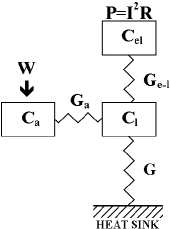
Figure 12: Thermal sketch of a bolometer or microcalorimeter in the case of absorber decoupling and hot electron model

Notice that these fluctuations transport power from the lattice system to the electron system and viceversa, therefore if a power $P_{he}$ adds to the electron system, the same power $P_{he}$ is subtracted from the lattice system. The effect is shown in the block diagram of Fig. 11. Solving the block diagram for the hot electron noise we obtain:

$$NEP_{he}=P_{he}\frac{G}{G_{\mathit{e-l}}(T_{l})}(1+j\omega\tau_{l}),$$ (82)

where $\tau_{l}$ has been previously defined as $\tau_{l}=C_{l}/G$. This expression does not depend on $C_{e}$, therefore is valid also for the case $C_{e}=0$. Moreover, if $G_{0e}\rightarrow\infty$, this term is zero, as expected.

IV Absorber Decoupling

Another aspect that may affect the performance of bolometers and microcalorimeters that we want to study is the effect of the absorber thermal conductivity. Most of the detectors are built with absorber and sensor as different entities connected by epoxy or other material with a thermal conductivity $G_{a}$. Depending on the experimental setup, there are different configurations that must be used to describe the thermal system. For example, the thermal link to the heat sink can be through the absorber or the thermometer and the absorber can be in thermal connection with the lattice system (when an electrical insulating material is used) or the electron system (when a conducting material is used).

What we want to analyze here is the case in which the detector is connected to the heat sink through the thermometer lattice system and the absorber is connected to the lattice system of the thermometer. In this case, the external power hits the absorber, is released to the lattice system and then detected in the electron system (see Fig. 12). We assume that the absorber has a heat capacity $C_{a}$. Notice that the analytical tools that we give here can be easily used to quantify the behavior of any other configuration.

IV.1 Responsivity and Dynamic Impedance

In equilibrium, with no other power input than the Joule power in the sensor, there is no power flow through the thermal link $G_{a}$ and therefore the temperature of the absorber is equal to the lattice temperature $T_{a}=T_{l}$. If an external power $W$ is applied to the absorber, the detector is described in the frequency domain by the set of equations:

$$j\omega C_{a}\Delta T_{a}+G_{a}\Delta T_{a}=W+G_{a}\Delta T_{l}$$ (83)

$$j\omega C_{l}\Delta T_{l}+(G+G_{a}+G_{\mathit{e-l}}(T_{l}))\Delta T_{l}=G_{a}\Delta T_{a}+G_{\mathit{e-l}}(T_{e})\Delta T_{e}$$ (84)

$$j\omega C_{e}\Delta T_{e}+G_{\mathit{e-l}}(T_{e})\Delta T_{e}=G_{\mathit{e-l}}(T_{l})\Delta T_{l}-G_{\mathit{ETF}}\Delta T_{e}.$$ (85)

If we want to build the block diagram associated with these three equations we can consider the left side of the equations as the response function of the three systems (absorber, lattice, electrons), and the right side as the input to each system. Connecting the three systems gives the block diagram of Fig. 13. The diagram can be solved to obtain the detector responsivity:

$$\begin{array}[]{c}S(\omega)=\frac{1}{j\omega C_{a}(1+j\omega\tau_{e})+(1+j\omega\tau_{e})(1+j\omega\tau_{a})(G+G_{\mathit{e-l}}(T_{l})+j\omega C_{l})-G_{\mathit{e-l}}(T_{e})A_{\mathit{e-l}}(1+j\omega\tau_{a})}\frac{A_{\mathit{e-l}}X\alpha A_{tr}}{T_{e}}\end{array}$$ (86)

with $\tau_{a}=C_{a}/G_{a}$. Notice that if $G_{a}\rightarrow\infty$ this expressions reduces to the one without absorber decoupling for a detector with lattice heat capacity $C_{l}=C_{l}+C_{a}$.

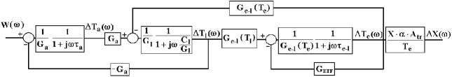
Figure 13: Block diagram representation of a detector with a finite thermal conductivity between absorber and lattice system. We have used the notation $G_{l}=G+G_{a}+G_{\mathit{e-l}}(T_{l})$. Notice that this implicitly integrates the heat relief for the lattice system provided by the electron and absorber decouling into the lattice response function. This is different from what was done before in Fig. 10, where the heat relief was explicitly reported in the block diagram as a feedback effect. The two descriptions are equivalent. We used the implicit description here to compact the block diagram algebra.

Using Eqs. 1, 23, 25, and 83 through 85, we can also calculate the detector dynamic impedance:

$$\begin{array}[]{c}Z(\omega)=R\frac{[(G+G_{\mathit{e-l}}(T_{l})+j\omega C_{l})(1+j\omega\tau_{a})+j\omega C_{a}]\left(G_{\mathit{e-l}}(T_{e})+j\omega C_{e}+\frac{P\alpha}{T_{e}}\right)-G_{\mathit{e-l}}(T_{e})\cdot G_{\mathit{e-l}}(T_{l})\cdot(1+j\omega\tau_{a})}{[(G+G_{\mathit{e-l}}(T_{l})+j\omega C_{l})(1+j\omega\tau_{a})+j\omega C_{a}]\left(G_{\mathit{e-l}}(T_{e})+j\omega C_{e}-\frac{P\alpha}{T_{e}}\right)-G_{\mathit{e-l}}(T_{e})\cdot G_{\mathit{e-l}}(T_{l})\cdot(1+j\omega\tau_{a})}\end{array}$$ (87)

IV.2 Noise contribution

As in the hot electron model of the thermometer, there are two effects introduced by the thermal link between the absorber and the lattice system. The first effect is that the response of the detector is different, therefore the $NEPs$ due to thermal, Johnson, $1/f$, load resistor, amplifier, and hot-electron noise are different. The second effect is the introduction of an extra noise term due to the power fluctuations between absorber and lattice.

Fig. 14 shows the block diagram of the detector with the noise sources evident. As in the hot electron model, the noise due to the link between absorber and lattice can be described as a power flow out of the absorber and into the lattice or viceversa. This power has same value $P_{a}$, but opposite sign at the two ends of the link. Since the temperature of absorber and lattice systems are equal, the value of $P_{a}$ is simply:

$$P_{a}=\sqrt{4k_{b}G_{a}T_{l}^{2}}.$$ (88)

Solving the block diagram of Fig. 14 independently for each noise source we obtain:

$$NEP_{th}=P_{th}(1+j\omega\tau_{a})$$ (89)

$$\begin{array}[]{c}NEP_{J}=\sqrt{\frac{4k_{b}T_{e}}{P\alpha^{2}}}\frac{T_{e}^{\beta_{e}+1}}{T_{l}^{\beta_{e}}}\left[(1+j\omega\tau_{\mathit{e-l}})\left(j\omega C_{a}+G(1+j\omega\tau_{a})(1+j\omega\tau_{l})\right)+(1+j\omega\tau_{a})\frac{T_{l}^{\beta_{e}}}{T_{e}^{\beta_{e}}}j\omega C_{e}\right]\end{array}$$ (90)

$$\begin{array}[]{rcl}NEP_{1/f}&=&\left(\frac{\Delta R}{R}\right)_{1/f}\frac{T_{e}}{\alpha}\frac{T_{e}^{\beta_{e}}}{T_{l}^{\beta_{e}}}\\ &\times&\left[(1+j\omega\tau_{\mathit{e-l}})\left(j\omega C_{a}+G(1+j\omega\tau_{a})(1+j\omega\tau_{l})\right)+(1+j\omega\tau_{a})\frac{T_{l}^{\beta_{e}}}{T_{e}^{\beta_{e}}}j\omega C_{e}\right]\end{array}$$ (91)

$$NEP_{R_{L}}=\frac{e_{R_{L}}}{S(\omega)}+\frac{2Ie_{R_{L}}}{G_{\mathit{e-l}}(T_{l})}\left[j\omega C_{a}+(1+j\omega\tau_{a})(G+G_{\mathit{e-l}}(T_{l})+j\omega C_{l})\right]$$ (92)

$$NEP_{amp}=e_{amp}/S(\omega)$$ (93)

$$NEP_{he}=\frac{P_{he}}{G_{\mathit{e-l}}(T_{l})}\left[j\omega C_{a}+G(1+j\omega\tau_{a})(1+j\omega\tau_{l})\right]$$ (94)

$$NEP_{a}=P_{a}j\omega\tau_{a}$$ (95)

Notice again that if $G_{a}\rightarrow\infty$ these expressions are equal to the hot-electron expressions for a detector with lattice heat capacity $C_{l}+C_{a}$ and the absorber $NEP$ is equal to zero.

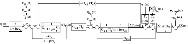
Figure 14: Block diagram representation of noise in a detector with a finite thermal conductivity between absorber and lattice system.

V Non-ohmic Behavior of the Thermometer

Another effect that may change the performance of a detector is the non-ohmic behavior of the thermometer, i.e., the thermometer resistance may not depend only on the thermometer electron temperature, but also on the current (or voltage) that is used to readout the temperature change: $R=R(T_{e},I)$ mather84 . This effect is particularly strong when TES thermometers are used mark . The responsivity of a detector with non-ohmic thermometer has already been calculated by J. C. Mather in 1984 mather84 and its effect on TES microcalorimeters has been studied in detail by M. A. Lindeman in 2000 mark . A non-ohmic thermometer can also be easily included in our model. If the resistance of the thermometer depends on the readout signal, we can write:

$$dR=\frac{R}{T_{e}}\alpha_{I}dT_{e}+\frac{R}{I}\beta_{I}dI$$ (96)

or equivalently

$$dR=\frac{R}{T_{e}}\alpha_{V}dT_{e}+\frac{R}{V}\beta_{V}dV,$$ (97)

where:

$$\alpha_{I}=\frac{T_{e}}{R}\frac{\partial R}{\partial T_{e}}\Bigg{|}_{I},\;\beta_{I}=\frac{I}{R}\frac{\partial R}{\partial I}\Bigg{|}_{T_{e}},\;\alpha_{V}=\frac{T_{e}}{R}\frac{\partial R}{\partial T_{e}}\Bigg{|}_{V},\;\mathrm{and}\;\beta_{V}=\frac{V}{R}\frac{\partial R}{\partial V}\Bigg{|}_{T_{e}}.$$ (98)

Using Eq. 96 or Eq. 97 is equivalent, and it is always possible to go from one notation to the other using Ohm’s laws:

$$\beta_{V}=\frac{\beta_{I}}{1+\beta_{I}}\;\mathrm{and}\;\alpha_{V}=\frac{\alpha_{I}}{1+\beta_{I}}.$$ (99)

The only terms in our model that are affected by the non-ohmic behavior are the electro-thermal feedback term $G_{\mathit{ETF}}$ and the transducer responsivity $A_{tr}$. We can calculate them assuming the bias circuit of Fig. 2.

$$P=I^{2}R\Rightarrow\Delta P=2IR\Delta I+I^{2}\Delta R,$$ (100)

$$I=\frac{V_{bias}}{R_{L}+R}\Rightarrow\Delta I=-\frac{I}{R_{L}+R}\Delta R,$$ (101)

and

$$V=V_{bias}-IR_{L}\Rightarrow\Delta V=-R_{L}\Delta I.$$ (102)

Using Eq. 96 we obtain:

$$\Delta P=-\frac{P}{T_{e}}\frac{R-R_{L}}{R_{L}+R(1+\beta_{I})}\alpha_{I}\Delta T_{e},$$ (103)

$$\frac{\Delta V}{V}=\alpha_{I}\frac{R_{L}}{R_{L}+R(1+\beta_{I})}\frac{\Delta T_{e}}{T_{e}},$$ (104)

and

$$\frac{\Delta I}{I}=-\alpha_{I}\frac{R}{R_{L}+R(1+\beta_{I})}\frac{\Delta T_{e}}{T_{e}}.$$ (105)

The model describing a non-ohmic thermometer is therefore identical to that describing a linear one, with the substitution:

$$\alpha\rightarrow\alpha_{I}$$ (106)

$$G_{\mathit{ETF}}=\frac{P}{T_{e}}\frac{R-R_{L}}{R_{L}+R(1+\beta_{I})}\alpha_{I},$$ (107)

and

$$A_{tr}=\frac{R_{L}}{R_{L}+R(1+\beta_{I})}$$ (108)

for voltage readout, or

$$A_{tr}=-\frac{R}{R_{L}+R(1+\beta_{I})}$$ (109)

for current readout. With this substitution in the equations that we derived previously in the paper, it is possible to predict both responsivity and noise in the detector.

We can also use Eq. 96 to calculate the dynamic impedance of the detector. In the case of absorber and hot-electron decoupling we obtain:

$$\begin{array}[]{rcl}Z(\omega)&=&R(\beta_{I}+1)\\ &\times&\frac{[(G+G_{\mathit{e-l}}(T_{l})+j\omega C_{l})(1+j\omega\tau_{a})+j\omega C_{a}]\left(G_{\mathit{e-l}}(T_{e})+j\omega C_{e}+\frac{P\alpha_{I}}{T_{e}(\beta_{I}+1)}\right)-G_{\mathit{e-l}}(T_{e})\cdot G_{\mathit{e-l}}(T_{l})\cdot(1+j\omega\tau_{a})}{[(G+G_{\mathit{e-l}}(T_{l})+j\omega C_{l})(1+j\omega\tau_{a})+j\omega C_{a}]\left(G_{\mathit{e-l}}(T_{e})+j\omega C_{e}-\frac{P\alpha_{I}}{T_{e}}\right)-G_{\mathit{e-l}}(T_{e})\cdot G_{\mathit{e-l}}(T_{l})\cdot(1+j\omega\tau_{a})}.\end{array}$$ (110)

This reduces to:

$$\begin{array}[]{c}Z(\omega)=R(\beta_{I}+1)\frac{(G+G_{\mathit{e-l}}(T_{l})+j\omega C_{l})\left(G_{\mathit{e-l}}(T_{e})+j\omega C_{e}+\frac{P\alpha_{I}}{T_{e}(\beta_{I}+1)}\right)-G_{\mathit{e-l}}(T_{e})\cdot G_{\mathit{e-l}}(T_{l})}{(G+G_{\mathit{e-l}}(T_{l})+j\omega C_{l})\left(G_{\mathit{e-l}}(T_{e})+j\omega C_{e}-\frac{P\alpha_{I}}{T_{e}}\right)-G_{\mathit{e-l}}(T_{e})\cdot G_{\mathit{e-l}}(T_{l})}\end{array}$$ (111)

for hot-electron decoupling only, and to:

$$Z(\omega)=R(\beta_{I}+1)\frac{1+\frac{P\alpha_{I}}{GT(\beta_{I}+1)}+j\omega\tau}{1-\frac{P\alpha_{I}}{GT}+j\omega\tau}$$ (112)

for the ideal model.

We do not know of a rigorous general method for deriving the Johnson noise in a non-ohmic resistor. Nor does there seem to be a single definite scheme for determining the net response of the detector to this fundamental thermal noise, since it is an internal noise generated in the non-ohmic resistor, and it is not clear how it should itself affect the non-ohmicity of the resistor. We are investigating this further, but for the present have assumed that the Johnson noise can be represented as a random voltage source with power spectral density $4k_{b}T_{e}R$ in series with the non-ohmic resistance, and that the Johnson fluctuations in the source cause the resistance to fluctuate due to the current dependence of the resistor. This results in the same suppression of the Johnson noise due to the current dependence of the resistance as occurs for external signals and noise if the non-ohmic resistance is expressed as $R(T_{e},I)$. This uncertainty (or dependence on the details of the physics) applies only to the Johnson noise of the sensor. Small-signal responsivities to all external sources of signal and noise are unambiguous, so it is only the detector Johnson noise contribution to the $NEP$ that is uncertain.

VI Results

To verify our results we simulated the performance of an existing microcalorimeter and compared the results with data from the detector. We considered a microcalorimeter used in the development phase of the X-Ray Spectrometer (XRS) for the Astro-E satellite xrs . The detector that we used for the comparison was part of a 6x6 test array of microcalorimeters with silicon implanted thermistors and HgTe absorbers. We chose this detector because the array has been studied in great detail and the characteristics of the pixels are well known.

We first used Eq. 37 and 38 to calculate the expected equilibrium temperature of the detector. We then used Eqs. 89 through 95 to calculated the expected noise spectra. The sum of these can be compared with the measured noise spectrum, as shown in Fig. 15. In the model all the input parameters are fixed to the values measured experimentally. The only value that was not available and that has been adjusted during the calculation of the theoretical noise is the stray capacitance between gate and source of the FET electronics. The value of 5 pF obtained for the stray capacitance is in good agreement with typical values for the FET amplifiers used in the measurement. The agreement between the model and the measurement is very good.

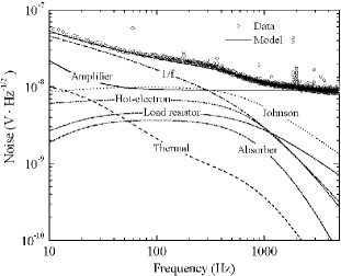
Figure 15: Comparison between the noise from a 6x6 XRS array pixel (courtesy of Caroline K. Stahle) and our model. The model includes the effect of the decoupling between hot electrons and phonons in the sensor and between absorber and sensor. The noise sources that are included are Johnson noise of the sensor, thermal noise due to the link between detector and heat sink, thermal noise due to the link between phonons and electrons in the sensor, thermal noise due to the link between absorber and sensor, Johnson noise of the load resistor, $1/f$ noise, and noise of the readout electronics.

The data set has been acquired at a heat sink temperature of 65 mK. The model predicts an equilibrium temperature of 77 mK and, through Eq. 69, an energy resolution of 8.4 eV, to be compared with the measured values of 78 mK and 8.65 eV. The agreement is well within the accuracy of the input parameters in the model and demonstrates the power of the model in predicting detector performance.

Our analytical model has also been compared with a model that uses matrix notation to numerically solve the linearized differential equations of the microcalorimeter tali . The numerical model was developed independently at the NASA/Goddard Space Flight Center to predict the performance of more complex detectors tali . Using the same parameter values, the agreement between the two is within the numerical error in the implementation of the models maxltd9 .

VII Conclusions

We have developed an analytical model that predicts the behavior of microcalorimeters and bolometers. The model includes the effect of hot electrons in the detector sensor, a thermal decoupling between absorber and sensor, and the effect of a non-ohmic thermometer. The model analytically predicts the detector responsivity and expected noise under these conditions. The noise sources that are included in the model are the Johnson noise of the sensor, the thermal noise due to the link between detector and heat sink, the thermal noise due to the link between phonons and electrons in the sensor, the thermal noise due to the link between absorber and sensor, the Johnson noise of the load resistor, the $1/f$ noise as thermal noise, and the noise of the readout electronics. A comparison between the predictions of our model and data from a detector developed for the XRS instrument shows good agreement.

We also described a different way to analyze the performance of bolometers and microcalorimeters, using block diagram algebra. The formalism that we introduced can be applied to the description of different detector configurations.

References

- (1) J. C. Mather, Appl. Opt. 21, 1125 (1982).
- (2) S. H. Moseley, J. C. Mather, and D. McCammon, J. Appl. Phys. 56, 1257 (1984).
- (3) H. F. .C. Hoevers, et al., Appl. Phys. Lett. 77, 4422 (2000).
- (4) J. M. Gildemeister, et al., Appl. Opt. 40, 6229 (2001).
- (5) A. Fleischmann, et al., AIP Conf. Proc. 605, 67 (2002), edited by F. S. Porter, D. McCammon, M. Galeazzi and C. K. Stahle.
- (6) M. Piat, et al., AIP Conf. Proc. 605, 79 (2002), edited by F. S. Porter, D. McCammon, M. Galeazzi and C. K. Stahle.
- (7) A. T. Lee, et al., IEEE Trans. Appl Supercon. 7, 2378 (1997).
- (8) M. J. M. E. de Nivelle, et al., J. Appl. Phys. 82, 4719 (1997).
- (9) M. Galeazzi, Rev. Sci. Instrum. 69, 2017 (1998).
- (10) Ning Wang, F. C. Wellstood, B. Saudolet, E. E. Haller, and J. Beeman, Phys. Rev. B 41, 3761 (1990).
- (11) J. Zhang, et al., Phys. Rev. B 57, 4472 (1998).
- (12) D. Liu, et al., AIP Conf. Proc. 605, 87 (2002), edited by F. S. Porter, D. McCammon, M. Galeazzi and C. K. Stahle.
- (13) M. Lindeman, Ph.D. Thesis, University of California at Davis (2000).
- (14) S-I Han, et al, Proc. SPIE 3445, 640 (1998), edited by O. H. Siegmund and M. A. Gummin.
- (15) W. S. Boyle and K. F. Rodgers Jr., J. Opt. Soc. Am. 49, 66 (1959).
- (16) S. R. Golwala, J. Jochum, and B. Saudolet, Proceedings of the Seventh International Workshop on Low Temperature Detectors, Munich, Germany, 27 July-2 August, edited by S. Cooper (The MAx Plank Institute, Munich, Germany, 1997) p. 64.
- (17) J. C. Mather, Appl. Opt. 23, 584 (1984).
- (18) C. K. Stahle, et al., Nucl. Instrum. Methods. Phys. Res. A 436, 218 (1999).
- (19) E. Figueroa-Feliciano, Ph.D. Thesis, Stanford University (2001).
- (20) M. Galeazzi, E. Figueroa-Feliciano, D. Liu, D. McCammon, W. T. Sanders, C. K. Stahle, and P. Tan, AIP Conf. Proc. 605, 95 (2002), edited by F. S. Porter, D. McCammon, M. Galeazzi and C. K. Stahle.