Chemical abundances of planet-host stars

In this paper, we present a study of the abundances of Si, Ca, Sc, Ti, V, Cr, Mn, Co, and Ni in a large set of stars known to harbor giant planets, as well as in a comparison sample of stars not known to have any planetary-mass companions. We have checked for possible chemical differences between planet hosts and field stars without known planets. Our results show that overall, and for a given value of [Fe/H], the abundance trends for the planet hosts are nearly indistinguishable from those of the field stars. In general, the trends show no discontinuities, and the abundance distributions of stars with giant planets are high [Fe/H] extensions to the curves traced by the field dwarfs without planets. The only elements that might present slight differences between the two groups of stars are V, Mn, and to a lesser extent Ti and Co. We also use the available data to describe galactic chemical evolution trends for the elements studied. When comparing the results with former studies, a few differences emerge for the high [Fe/H] tail of the distribution, a region that is sampled with unprecedented detail in our analysis.

1 Introduction

Stars with planetary companions have been shown to be, on average, considerably metal-rich when compared with stars in the solar neighborhood (e.g. Gonzalez 1997; Fuhrmann et al. 1997; Gonzalez 1998; Sadakane et al. 1999; Santos et al. 2000; Gonzalez et al. 2001; Santos et al. 2001, 2003). The most recent results suggest indeed that the efficiency of planetary formation seems to be strongly dependent on the metal content of the cloud that gave origin to the star and planetary system.

Until now, however, most chemical studies of the planet hosts used iron as the reference element. The few systematic studies in the literature concerning other metals (Gonzalez 1997; Sadakane et al. 1999; Gonzalez & Laws 2000; Santos et al. 2000; Sadakane et al. 2001; Gonzalez et al. 2001; Smith et al. 2001; Sadakane et al. 2002) revealed a few possible (but not clear) anomalies. The situation concerning the light elements (in particular Li and Be – García López & Perez de Taoro 1998; Deliyannis et al. 2000; Gonzalez & Laws 2000; Ryan 2000; Gonzalez et al. 2001; Israelian et al. 2001; Santos et al. 2002; Reddy et al. 2002; Israelian et al. 2003) is not very different; the debate is just beginning to heat up and many questions remain open.

In almost every case, the authors have been constrained to compare the results for the star-with-planet samples with other studies in the literature concerning stars without known planetary companions. This might have introduced undesirable systematic errors, given that the different studies have not used the same set of spectral lines and model atmospheres to derive the stellar parameters and abundances. How important are the systematic differences between the various studies? And how can these differences lead to mistakes? A systematic comparison between two groups of stars (with and without planetary companions) is thus needed.

To try to fill (at least in part) this gap, we present in this paper a detailed and uniform study of the elements Si, Ca, Sc, Ti, V, Cr, Mn, Co, and Ni in a large sample of planet-host stars, and in a “comparison” volume-limited sample of stars not known to have any planetary-mass companions. In Sect.2, we present our samples as well as the chemical analysis, and in Sect.3 we compare the abundances. The results seem to indicate that no clearly significant differences exist between the two groups of stars. In Sect.4, we use the current data to explore the galactic chemical evolution trends. Given the high metal content of many stars in our sample, we could access the high [Fe/H] tail of the distributions with unprecedented detail. We conclude in Sect.5.

2 Data, atmospheric parameters, and chemical analysis

2.1 The data

In a series of recent papers (Santos et al. 2000, 2001, 2003), we have been gathering spectra for most of the planet-host stars known today. This data has been used to derive precise and uniform stellar parameters for the target stars, as well as accurate iron abundances. The results published to this point have been used to show that stars with planets are substantially metal-rich when compared with average field dwarfs.

The current paper employs the same spectra and stellar parameters derived in these works. This allowed access to elemental abundances for 77 stars with low-mass companions (planetary or brown-dwarf candidates).

Spectra for the comparison sample used in this work were obtained with the main goal of deriving the metallicities for a large sample of stars in a limited volume around the Sun and not known to harbor any planetary-mass companions (Santos et al. 2001). With the exception of HD 39091 (that was, in the meanwhile, found to have a brown-dwarf candidate companion – (Jones et al. 2002)), the comparison sample used here consists of the remaining 42 objects in Table 1 of Santos et al. (2001). This sample is indeed perfect and appropriate for the current work, as its stellar parameters and iron abundances have been derived using the same methods as those used for all the planet hosts analyzed in this paper.

We should caution that this comparison sample is built from a list of stars that are surveyed for planets, but for which none have yet been found. Of course, this does not mean that these stars do not have any planetary mass companions at all (they might have e.g. very low mass and/or long period planets which are more difficult to detect with radial-velocity surveys). However, the odds that planets similar to the ones found to date are present among these stars are not very high.

In the rest of the paper, all the stellar parameters and [Fe/H] values have been taken from the uniform studies of Santos et al. (2000, 2001, 2003) for both samples. For more details on the reduction and analysis we refer to these works.

2.2 Chemical Analysis

Abundances for all the elements studied here were derived in standard Local Thermodynamic Equilibrium (LTE) using a revised version of the code MOOG (Sneden 1973), and a grid of Kurucz (1993) ATLAS9 atmospheres. For each element, a set of (weak) lines was chosen from the literature, with wavelengths between about 5000 and 6800Å (the usual spectral domain of our data). Then, using the Kurucz Solar Atlas (Kurucz et al. 1984), we verified each line to check for possible blends. Only isolated lines were taken; for these, the solar equivalent widths (EW) were measured.

Table 1: Spectral lines of the elements used in this experiment. Col. 1: wavelength (in Ångstroms). Col. 2: excitation energy of the lower energy level in the transition (in eV). Col. 3: oscillator strengths based on an inverse solar analysis.

$\lambda$	$\chi_{l}$	$\log{gf}$		$\lambda$	$\chi_{l}$	$\log{gf}$
Si I ; $\log\epsilon_{\circ}=7.55$ A $=$ 14				6261.11	1.43	$-$0.4881
5665.56	4.92	$-$1.9788		6303.76	1.44	$-$1.6003
5690.43	4.93	$-$1.7878		6312.24	1.46	$-$1.5850
5701.10	4.93	$-$2.0227		V I ; $\log\epsilon_{\circ}=4.00$ A $=$ 23
5772.14	5.08	$-$1.6179		5727.05	1.08	$-$0.0004
5793.09	4.93	$-$1.9134		6090.21	1.08	$-$0.1549
5948.55	5.08	$-$1.1135		6216.35	0.28	$-$0.8996
6125.02	5.61	$-$1.5157		6452.31	1.19	$-$0.8239
6142.49	5.62	$-$1.4788		6531.42	1.22	$-$0.9208
6145.02	5.61	$-$1.4012		Cr I ; $\log\epsilon_{\circ}=5.67$ A $=$ 24
6155.15	5.62	$-$0.7520		5304.18	3.46	$-$0.6777
6721.86	5.86	$-$1.0872		5312.86	3.45	$-$0.5850
Ca I ; $\log\epsilon_{\circ}=6.36$ A $=$ 20				5318.77	3.44	$-$0.7099
5512.98	2.93	$-$0.4377		5480.51	3.50	$-$0.8268
5581.97	2.52	$-$0.6536		5574.39	4.45	$-$0.4814
5590.12	2.52	$-$0.7077		5783.07	3.32	$-$0.4034
5867.56	2.93	$-$1.5900		5783.87	3.32	$-$0.1487
6161.29	2.52	$-$1.2182		5787.92	3.32	$-$0.1067
6166.44	2.52	$-$1.1163		Mn I ; $\log\epsilon_{\circ}=5.39$ A $=$ 25
6169.05	2.52	$-$0.7328		5388.50	3.37	$-$1.6289
6169.56	2.52	$-$0.4436		5399.47	3.85	$-$0.0969
6449.82	2.52	$-$0.6289		6440.93	3.77	$-$1.2518
6455.60	2.52	$-$1.3736		Co I ; $\log\epsilon_{\circ}=4.92$ A $=$ 27
Sc II ; $\log\epsilon_{\circ}=3.10$ A $=$ 21				5301.04	1.71	$-$1.9318
5239.82	1.45	$-$0.7594		5312.65	4.21	$-$0.0199
5318.36	1.36	$-$1.6989		5483.36	1.71	$-$1.2182
5526.82	1.77	0.14612		6455.00	3.63	$-$0.2839
6245.62	1.51	$-$1.0409		6632.44	2.28	$-$1.8827
6300.69	1.51	$-$1.9586		Ni I ; $\log\epsilon_{\circ}=6.25$ A $=$ 28
6320.84	1.50	$-$1.8386		5578.72	1.68	$-$2.6517
6604.60	1.36	$-$1.1611		5587.86	1.93	$-$2.3819
Ti I ; $\log\epsilon_{\circ}=4.99$ A $=$ 22				5682.20	4.10	$-$0.3872
5471.20	1.44	$-$1.5528		5694.99	4.09	$-$0.6020
5474.23	1.46	$-$1.3615		5805.22	4.17	$-$0.5767
5490.15	1.46	$-$0.9829		5847.00	1.68	$-$3.4089
5866.46	1.07	$-$0.8386		6086.28	4.26	$-$0.4436
6091.18	2.27	$-$0.4559		6111.07	4.09	$-$0.8013
6126.22	1.07	$-$0.4145		6128.98	1.68	$-$3.3665
6258.11	1.44	$-$0.4365		6130.14	4.26	$-$0.9469

Table 2: Sensitivity of the derived abundances to changes of 0.10 dex in metallicity, 0.15 dex in gravity, 0.10 km s^-1 in microturbulence, and 50 K in effective temperature for the K dwarf HD 50281 A, for a solar-type star (HD 43162), and for the late-F dwarf HD 10647.

Star	Si	Ca	Sc	Ti	V	Cr	Mn	Co	Ni
HD 50281A	($[$Fe$/$H$]$ ; $\log\,g$ ; $\xi_{t}$ ; Teff) = (0.07 ; 4.75 ; 0.85 ; 4790)
$\Delta[$Fe$/$H$]=+$0.10 dex	0.03	0.02	0.04	0.01	0.02	0.02	0.02	0.03	0.03
$\Delta\log\,g=+$0.15 dex	0.03	0.02	0.06	$-$0.02	$-$0.03	$-$0.01	0.00	0.03	0.02
$\Delta\xi_{t}=+$0.10 km$\cdot$s-1	0.00	$-$0.01	$-$0.01	$-$0.03	$-$0.04	$-$0.01	$-$0.01	$-$0.02	$-$0.02
$\Delta$ T${}_{\mathrm{eff}}=+$50 K	$-$0.02	0.05	$-$0.01	0.06	0.06	0.03	0.01	0.01	$-$0.01
HD 43162	($[$Fe$/$H$]$ ; $\log\,g$ ; $\xi_{t}$ ; Teff) = ($-$0.02 ; 4.57 ; 1.36 ; 5630)
$\Delta[$Fe$/$H$]=+$0.10 dex	0.01	0.00	0.03	0.00	$-$0.01	0.00	0.00	0.01	0.01
$\Delta\log\,g=+$0.15 dex	0.01	$-$0.04	0.06	0.00	$-$0.01	$-$0.01	0.00	0.01	0.01
$\Delta\xi_{t}=+$0.10 km$\cdot$s-1	$-$0.01	$-$0.03	$-$0.01	$-$0.01	$-$0.02	$-$0.01	$-$0.01	$-$0.01	$-$0.01
$\Delta$ T${}_{\mathrm{eff}}=+$50 K	0.00	0.03	0.00	0.05	0.05	0.03	0.03	0.04	0.03
HD 10647	($[$Fe$/$H$]$ ; $\log\,g$ ; $\xi_{t}$ ; Teff) = ($-$0.03 ; 4.45 ; 1.31 ; 6130)
$\Delta[$Fe$/$H$]=+$0.10 dex	0.00	$-$0.01	0.02	0.00	0.00	0.00	$-$0.01	0.00	0.00
$\Delta\log\,g=+$0.15 dex	0.00	$-$0.02	0.06	0.00	0.00	0.00	$-$0.01	0.00	0.00
$\Delta\xi_{t}=+$0.10 km$\cdot$s-1	$-$0.01	$-$0.02	$-$0.02	0.00	0.00	$-$0.01	$-$0.01	$-$0.01	$-$0.01
$\Delta$ T${}_{\mathrm{eff}}=+$50 K	0.01	0.03	0.01	0.04	0.05	0.03	0.02	0.04	0.03

Using these measured EW values and a solar atmosphere with (T_eff,$\log{g}$,$\xi_{t}$)=(5770 K,4.44 dex,1.00 km s^-1), we have derived $\log{gf}$ values for the individual lines from an inverted solar analysis (using the ewfind driver in MOOG). The solar abundances were taken from Anders & Grevesse (1989). In order to do the subsequent chemical analysis for our targets in a reasonable amount of time, we reduced the number of lines per element to a maximum of $\sim$10. The final list of lines used is presented in Table 1.

For each line in our targets, the EW was measured using the IRAF splot tool, and the abundances were computed using MOOG with the abfind driver. The average of the abundances for the lines of a given element was then considered. In Tables 3, 4, 5, and 6 we summarize the derived abundances for all stars with and without planetary-mass companions. The uncertainties in the tables denote the rms around the mean. The number of lines used in each case is also noted.

We remark that in particular cases, some lines were eliminated from the analysis when the quality of the spectrum in the region of interest was not good enough to permit a reliable EW measurement (e.g. lower than usual S/N or the presence of cosmic-rays).

2.3 Uncertainties

Uncertainties can sway the abundances in various ways. For example, errors can affect individual lines with random errors in the EWs, oscillator strengths and damping constants. Systematic errors in the EWs can arise from unnoticed blends or a poor location of the continuum. These errors are hard to spot, but they are minimized thanks to the normally high quality of our data. Atmospheric parameter uncertainties should be the primary source of abundance error in a species with many lines, whereas inaccuracies in the EWs are eventually more important when only a few lines are available.

Assuming perturbations of 0.10 dex in the overall metallicity (scaled with [Fe/H]), 0.15 dex in $\log g$, 0.10 km s^-1 in $\xi_{t}$, and 50 K in effective temperatures (usual values for our sample), this leads to a total typical uncertainty of about 0.05 dex in the [X/H] abundance ratios (see Table 2) using the lines listed in Table 1. Adding quadratically to the abundance dispersions for each element, we estimate that the errors in the abundances derived here are usually lower than 0.10 dex.

Table 3: Atmospheric parameters (taken from Santos et al. 2001, 2003) and abundances derived for Si, Ca, Sc, and Ti for the stars with giant planets studied in this paper. All the abundances are expressed as [X/H]=$\log{N(\mathrm{X})/N(\mathrm{H})}$+12. The number of spectral lines used is given by $n$, while $\sigma$ denotes the rms around the average.

Star	Teff	$\log g$	$\xi_{t}$	Fe	Si	$\sigma$	$n$	Ca	$\sigma$	$n$	Sc	$\sigma$	$n$	Ti	$\sigma$	$n$
HD 142	6290	4.38	1.91	0.11	0.14	0.04	10	0.08	0.08	10	0.10	0.07	4	0.03	0.04	2
HD 1237	5555	4.65	1.50	0.11	0.06	0.06	11	0.09	0.07	10	0.08	0.09	5	0.12	0.06	9
HD 2039	5990	4.56	1.24	0.34	0.33	0.03	11	0.29	0.05	10	0.36	0.05	5	0.33	0.04	8
HD 4203	5650	4.38	1.15	0.40	0.44	0.05	11	0.33	0.07	10	0.48	0.07	6	0.39	0.09	10
HD 4208	5625	4.54	0.95	$-$0.23	$-$0.20	0.05	11	$-$0.20	0.03	10	$-$0.18	0.08	5	$-$0.17	0.07	10
HD 6434	5790	4.56	1.40	$-$0.55	$-$0.34	0.05	11	$-$0.40	0.04	10	$-$0.33	0.08	5	$-$0.32	0.06	6
HD 8574	6080	4.41	1.25	0.05	$-$0.02	0.04	11	0.01	0.08	6	0.12	0.07	4	$-$0.05	0.04	3
HD 9826	6120	4.07	1.50	0.10	0.12	0.04	9	0.16	0.08	5	0.08	0.09	3	0.08	0.00	1
HD 10697	5665	4.18	1.19	0.14	0.14	0.02	11	0.09	0.04	7	0.23	0.09	6	0.12	0.03	9
HD 12661	5715	4.49	1.09	0.36	0.35	0.05	11	0.23	0.12	9	0.49	0.13	6	0.30	0.04	7
HD 13445	5205	4.70	0.82	$-$0.20	$-$0.14	0.05	11	$-$0.19	0.07	9	$-$0.12	0.12	6	$-$0.01	0.08	10
HD 16141	5805	4.28	1.37	0.15	0.10	0.03	11	0.09	0.03	10	0.22	0.09	7	0.13	0.04	9
HD 17051	6225	4.65	1.20	0.25	0.20	0.04	11	0.23	0.05	10	0.24	0.06	6	0.20	0.08	6
HD 19994	6175	4.14	1.52	0.21	0.22	0.08	11	0.22	0.07	8	0.20	0.12	4	0.15	0.05	4
HD 20367	6100	4.55	1.31	0.14	0.06	0.08	11	0.05	0.06	10	0.01	0.11	5	$-$0.01	0.14	6
HD 22049	5135	4.70	1.14	$-$0.07	$-$0.10	0.05	11	$-$0.10	0.07	9	$-$0.07	0.16	5	0.00	0.04	10
HD 23079	5945	4.44	1.21	$-$0.11	$-$0.14	0.05	11	$-$0.08	0.05	10	$-$0.12	0.13	7	$-$0.11	0.05	7
HD 23596	6125	4.29	1.32	0.32	0.30	0.03	11	0.27	0.05	9	0.33	0.01	5	0.28	0.05	9
HD 27442	4890	3.89	1.24	0.42	0.46	0.13	11	0.18	0.09	8	0.57	0.12	6	0.39	0.09	9
HD 28185	5705	4.59	1.09	0.24	0.23	0.04	11	0.16	0.04	10	0.35	0.09	6	0.23	0.05	8
HD 30177	5590	4.45	1.07	0.39	0.41	0.07	11	0.23	0.07	10	0.52	0.20	7	0.32	0.09	10
HD 33636	5990	4.68	1.22	$-$0.05	$-$0.06	0.04	11	$-$0.04	0.03	10	0.04	0.09	5	$-$0.03	0.08	7
HD 37124	5565	4.62	0.90	$-$0.37	$-$0.24	0.06	11	$-$0.28	0.05	10	$-$0.16	0.10	5	$-$0.14	0.05	8
HD 38529	5675	4.01	1.39	0.39	0.39	0.05	11	0.32	0.05	10	0.43	0.04	6	0.37	0.05	10
HD 39091	5995	4.48	1.30	0.09	0.08	0.02	11	0.05	0.02	10	0.13	0.05	7	0.05	0.04	9
HD 46375	5315	4.54	1.11	0.21	0.21	0.06	11	0.14	0.10	10	0.21	0.08	5	0.28	0.07	10
HD 50554	6050	4.59	1.19	0.02	$-$0.01	0.06	11	0.01	0.06	10	0.10	0.06	5	0.03	0.05	6
HD 52265	6098	4.29	1.31	0.24	0.22	0.04	11	0.21	0.05	10	0.21	0.06	5	0.18	0.03	6
HD 74156	6105	4.40	1.36	0.15	0.13	0.03	11	0.12	0.07	10	0.19	0.00	4	0.10	0.03	7
HD 75289	6135	4.43	1.50	0.27	0.22	0.04	11	0.24	0.04	10	0.27	0.10	5	0.22	0.03	6
HD 75732	5307	4.58	1.06	0.35	0.38	0.06	11	0.19	0.09	10	0.40	0.10	6	0.38	0.11	10
HD 80606	5570	4.56	1.11	0.34	0.36	0.04	11	0.22	0.09	10	0.40	0.11	6	0.36	0.07	10
HD 82943	6025	4.54	1.12	0.32	0.31	0.07	11	0.24	0.03	10	0.30	0.05	6	0.24	0.05	10
HD 83443	5500	4.50	1.12	0.39	0.44	0.07	11	0.25	0.10	10	0.41	0.09	6	0.38	0.07	10
HD 92788	5820	4.60	1.12	0.34	0.32	0.03	11	0.25	0.05	10	0.44	0.11	7	0.35	0.03	10
HD 95128	5925	4.45	1.24	0.05	0.01	0.08	11	0.01	0.03	6	0.09	0.04	6	0.04	0.03	10
HD 106252	5890	4.40	1.06	$-$0.01	$-$0.07	0.04	11	$-$0.06	0.03	10	$-$0.04	0.10	7	$-$0.10	0.06	9
HD 108147	6265	4.59	1.40	0.20	0.14	0.03	11	0.14	0.02	10	0.20	0.08	4	0.10	0.03	4
HD 108874	5615	4.58	0.93	0.25	0.21	0.04	11	0.12	0.05	8	0.36	0.10	6	0.23	0.09	9
HD 114386	4875	4.69	0.63	0.00	0.00	0.06	11	$-$0.06	0.13	10	0.11	0.07	4	0.20	0.09	10
HD 114729	5820	4.20	1.03	$-$0.26	$-$0.24	0.03	10	$-$0.23	0.05	8	$-$0.06	0.11	6	$-$0.18	0.04	6
HD 114762	5870	4.25	1.28	$-$0.72	$-$0.57	0.02	8	$-$0.57	0.05	10	$-$0.61	0.06	7	$-$0.58	0.08	9
HD 114783	5160	4.75	0.79	0.16	0.14	0.05	10	$-$0.03	0.10	6	0.27	0.05	6	0.25	0.08	10
HD 117176	5530	4.05	1.08	$-$0.05	$-$0.07	0.09	11	$-$0.06	0.03	7	0.02	0.09	7	$-$0.03	0.03	10
HD 121504	6090	4.73	1.35	0.17	0.12	0.03	11	0.09	0.03	10	0.19	0.09	5	0.17	0.04	6
HD 128311	4950	4.80	1.00	0.10	0.07	0.07	10	$-$0.04	0.12	8	0.15	0.13	5	0.16	0.09	9
HD 130322	5430	4.62	0.92	0.06	0.02	0.08	10	0.01	0.06	6	0.09	0.12	7	0.11	0.04	10
HD 134987	5780	4.45	1.06	0.32	0.32	0.03	10	0.23	0.03	6	0.45	0.11	7	0.31	0.03	10
HD 136118	6175	4.18	1.61	$-$0.06	$-$0.08	0.06	10	$-$0.03	0.08	6	$-$0.13	0.13	7	$-$0.15	0.12	5
HD 137759	4750	3.15	1.78	0.09	0.12	0.06	9	$-$0.09	0.14	6	0.28	0.05	5	0.18	0.13	9
HD 141937	5925	4.62	1.16	0.11	0.15	0.04	11	0.10	0.03	10	0.18	0.13	7	0.11	0.07	10
HD 143761	5835	4.40	1.29	$-$0.21	$-$0.15	0.04	10	$-$0.17	0.03	6	$-$0.05	0.06	7	$-$0.11	0.06	10
HD 145675	5255	4.40	0.68	0.51	0.49	0.09	10	0.29	0.10	6	0.51	0.13	6	0.44	0.08	8
HD 147513	5880	4.58	1.17	0.07	$-$0.01	0.03	11	0.08	0.04	10	0.04	0.10	6	0.03	0.03	9
HD 150706	6000	4.62	1.16	0.01	$-$0.06	0.03	10	$-$0.03	0.04	8	$-$0.04	0.08	5	$-$0.05	0.07	8
HD 160691	5820	4.44	1.23	0.33	0.32	0.03	11	0.22	0.03	10	0.38	0.04	6	0.31	0.04	10
HD 162020	4830	4.76	0.72	0.01	$-$0.08	0.07	8	$-$0.15	0.11	8	$-$0.12	0.22	4	0.09	0.09	10
HD 168443	5600	4.30	1.18	0.06	0.08	0.05	10	0.02	0.04	6	0.19	0.03	4	0.13	0.02	9
HD 168746	5610	4.50	1.02	$-$0.06	0.01	0.04	11	$-$0.03	0.06	10	0.09	0.15	5	0.08	0.04	8
HD 169830	6300	4.04	1.37	0.22	0.15	0.03	11	0.18	0.08	10	0.15	0.12	6	0.09	0.02	6
HD 177830	4840	3.60	1.18	0.32	0.35	0.06	8	0.17	0.11	8	0.38	0.10	5	0.33	0.12	9
HD 179949	6235	4.41	1.38	0.21	0.16	0.05	8	0.20	0.07	8	0.11	0.07	4	0.10	0.02	3
HD 186427	5765	4.46	1.03	0.09	0.04	0.06	10	0.04	0.02	6	0.16	0.10	7	0.06	0.04	9
HD 187123	5855	4.48	1.10	0.14	0.06	0.07	11	0.08	0.02	6	0.15	0.11	7	0.08	0.05	10
HD 190228	5340	3.99	1.11	$-$0.24	$-$0.23	0.02	11	$-$0.24	0.03	6	$-$0.12	0.08	7	$-$0.15	0.02	9
HD 190360	5590	4.48	1.06	0.25	0.26	0.04	11	0.14	0.08	8	0.41	0.13	6	0.28	0.05	8
HD 192263	4995	4.76	0.90	0.04	0.02	0.07	10	$-$0.06	0.11	10	0.09	0.16	5	0.11	0.09	10
HD 195019	5840	4.36	1.24	0.08	0.04	0.02	11	0.05	0.03	10	0.15	0.08	6	0.10	0.04	8
HD 196050	5905	4.41	1.40	0.21	0.23	0.03	11	0.13	0.02	10	0.33	0.08	6	0.17	0.06	10
HD 202206	5765	4.75	0.99	0.37	0.30	0.03	11	0.24	0.03	10	0.45	0.04	4	0.28	0.04	7
HD 209458	6120	4.56	1.37	0.02	0.01	0.03	9	0.01	0.02	10	0.07	0.06	7	$-$0.02	0.06	8
HD 210277	5570	4.45	1.08	0.22	0.23	0.04	11	0.20	0.08	10	0.23	0.10	6	0.27	0.04	10
HD 213240	5975	4.32	1.30	0.16	0.12	0.04	11	0.09	0.04	10	0.24	0.08	6	0.11	0.04	6
HD 216435	5905	4.16	1.26	0.22	0.19	0.04	11	0.14	0.06	10	0.20	0.05	5	0.11	0.04	7
HD 216437	5875	4.38	1.30	0.25	0.22	0.03	11	0.16	0.03	10	0.33	0.12	7	0.17	0.03	10
HD 217014	5805	4.51	1.22	0.21	0.21	0.04	11	0.12	0.03	9	0.29	0.09	7	0.18	0.05	9
HD 217107	5658	4.43	1.08	0.39	0.37	0.04	11	0.28	0.07	10	0.46	0.13	5	0.34	0.04	10
HD 222582	5850	4.58	1.06	0.06	0.00	0.05	9	$-$0.10	0.15	9	0.08	0.10	5	$-$0.03	0.10	4

Table 4: Same as Table 3 but for V, Cr, Mn, Co, and Ni.

Star	Teff	V	$\sigma$	$n$	Cr	$\sigma$	$n$	Mn	$\sigma$	$n$	Co	$\sigma$	$n$	Ni	$\sigma$	$n$
HD 142	6290	0.08	0.00	1	0.05	0.05	3	–	–	0	–	–	0	0.03	0.06	4
HD 1237	5555	0.11	0.07	3	0.12	0.05	6	0.18	0.10	2	0.01	0.03	3	0.07	0.04	10
HD 2039	5990	0.34	0.12	4	0.33	0.05	6	0.50	0.00	1	0.45	0.04	3	0.35	0.06	10
HD 4203	5650	0.40	0.07	4	0.36	0.06	7	0.54	0.17	2	0.54	0.01	3	0.45	0.05	9
HD 4208	5625	$-$0.29	0.10	4	$-$0.28	0.05	7	$-$0.41	0.00	1	$-$0.29	0.00	3	$-$0.23	0.05	10
HD 6434	5790	$-$0.45	0.07	3	$-$0.55	0.03	4	–	–	0	$-$0.51	0.09	2	$-$0.54	0.05	10
HD 8574	6080	$-$0.08	0.00	2	$-$0.06	0.03	6	$-$0.18	0.00	1	$-$0.09	0.19	2	$-$0.03	0.03	9
HD 9826	6120	$-$0.05	0.01	2	0.03	0.02	3	$-$0.02	0.00	1	–	–	0	0.02	0.07	4
HD 10697	5665	0.14	0.09	4	0.11	0.03	7	0.12	0.09	2	0.15	0.09	5	0.11	0.05	10
HD 12661	5715	0.38	0.07	5	0.31	0.06	7	0.50	0.16	2	0.48	0.05	4	0.36	0.07	10
HD 13445	5205	$-$0.06	0.01	3	$-$0.19	0.05	7	$-$0.39	0.05	2	$-$0.07	0.08	4	$-$0.21	0.06	10
HD 16141	5805	0.12	0.02	4	0.16	0.05	7	0.05	0.09	2	0.14	0.06	4	0.10	0.05	10
HD 17051	6225	0.24	0.07	3	0.21	0.06	4	0.25	0.00	1	$-$0.02	0.12	2	0.19	0.03	10
HD 19994	6175	0.17	0.09	3	0.14	0.01	3	0.13	0.00	1	–	–	0	0.20	0.05	7
HD 20367	6100	0.07	0.06	3	0.09	0.05	4	0.00	0.00	1	$-$0.21	0.00	1	$-$0.02	0.09	10
HD 22049	5135	0.07	0.11	4	$-$0.09	0.03	8	$-$0.09	0.11	2	$-$0.09	0.10	5	$-$0.16	0.04	10
HD 23079	5945	$-$0.22	0.03	3	$-$0.19	0.05	6	$-$0.28	0.00	1	$-$0.30	0.09	3	$-$0.18	0.06	10
HD 23596	6125	0.37	0.11	5	0.27	0.04	7	0.31	0.00	1	0.34	0.09	3	0.32	0.07	10
HD 27442	4890	0.65	0.14	3	0.25	0.04	7	0.69	0.30	2	0.84	0.08	4	0.45	0.11	9
HD 28185	5705	0.31	0.07	3	0.24	0.03	7	0.42	0.00	1	0.38	0.09	4	0.31	0.04	10
HD 30177	5590	0.45	0.13	3	0.34	0.03	7	0.41	0.34	2	0.56	0.16	4	0.38	0.09	10
HD 33636	5990	$-$0.09	0.06	3	$-$0.12	0.05	4	$-$0.28	0.00	1	$-$0.17	0.10	2	$-$0.12	0.06	10
HD 37124	5565	$-$0.30	0.11	3	$-$0.46	0.06	7	$-$0.72	0.00	1	$-$0.31	0.02	2	$-$0.42	0.05	10
HD 38529	5675	0.40	0.02	3	0.34	0.07	7	0.33	0.00	1	0.55	0.11	4	0.40	0.06	10
HD 39091	5995	0.07	0.08	3	0.05	0.05	6	0.06	0.00	1	0.04	0.09	2	0.08	0.04	10
HD 46375	5315	0.34	0.04	3	0.21	0.05	7	0.41	0.23	2	0.42	0.14	5	0.24	0.03	9
HD 50554	6050	$-$0.06	0.05	3	$-$0.04	0.05	6	$-$0.15	0.00	1	$-$0.01	0.30	2	$-$0.04	0.04	10
HD 52265	6098	0.18	0.07	3	0.20	0.04	5	0.17	0.00	1	0.06	0.01	2	0.21	0.04	10
HD 74156	6105	0.11	0.08	3	0.08	0.04	6	0.02	0.00	1	0.07	0.11	2	0.13	0.04	10
HD 75289	6135	0.25	0.09	3	0.19	0.02	3	0.15	0.00	1	0.12	0.02	2	0.21	0.04	10
HD 75732	5307	0.52	0.08	3	0.29	0.04	8	0.53	0.27	2	0.64	0.16	4	0.39	0.09	10
HD 80606	5570	0.47	0.19	5	0.35	0.07	7	0.52	0.11	2	0.52	0.14	5	0.40	0.06	9
HD 82943	6025	0.30	0.08	4	0.25	0.03	7	0.29	0.09	2	0.21	0.05	5	0.31	0.04	10
HD 83443	5500	0.46	0.05	3	0.32	0.06	8	0.64	0.27	2	0.56	0.17	5	0.42	0.07	10
HD 92788	5820	0.40	0.05	5	0.30	0.05	8	0.40	0.11	3	0.42	0.10	5	0.37	0.06	10
HD 95128	5925	0.05	0.05	3	0.02	0.05	7	0.04	0.07	2	$-$0.02	0.06	5	0.04	0.04	9
HD 106252	5890	$-$0.11	0.05	3	$-$0.09	0.02	5	$-$0.14	0.00	1	$-$0.10	0.12	2	$-$0.09	0.04	10
HD 108147	6265	0.18	0.11	3	0.13	0.03	3	–	–	0	–	–	0	0.10	0.04	8
HD 108874	5615	0.23	0.11	4	0.20	0.08	6	0.24	0.08	3	0.27	0.21	5	0.27	0.06	9
HD 114386	4875	0.34	0.14	4	$-$0.04	0.07	8	0.11	0.12	3	0.16	0.20	5	0.02	0.09	10
HD 114729	5820	$-$0.25	0.17	4	$-$0.33	0.10	6	$-$0.49	0.00	1	$-$0.38	0.13	4	$-$0.31	0.04	9
HD 114762	5870	$-$0.71	0.06	3	$-$0.87	0.22	2	$-$1.18	0.00	1	$-$0.87	0.08	4	$-$0.75	0.04	9
HD 114783	5160	0.33	0.01	2	0.11	0.03	8	0.27	0.19	2	0.32	0.08	4	0.19	0.08	10
HD 117176	5530	$-$0.07	0.07	4	$-$0.11	0.03	7	$-$0.16	0.00	1	$-$0.08	0.10	5	$-$0.10	0.03	9
HD 121504	6090	0.18	0.07	3	0.14	0.04	6	0.12	0.00	1	0.09	0.10	2	0.13	0.05	10
HD 128311	4950	0.25	0.09	2	0.03	0.10	6	0.16	0.09	3	0.21	0.09	4	0.05	0.11	9
HD 130322	5430	0.12	0.18	4	0.06	0.03	8	0.10	0.09	2	0.11	0.13	5	0.06	0.04	10
HD 134987	5780	0.35	0.07	4	0.28	0.03	8	0.29	0.26	3	0.41	0.13	5	0.36	0.04	10
HD 136118	6175	$-$0.20	0.00	2	$-$0.07	0.05	3	$-$0.24	0.00	1	–	–	0	$-$0.14	0.04	8
HD 137759	4750	0.29	0.09	3	0.08	0.10	8	0.23	0.02	2	0.47	0.21	5	0.11	0.15	9
HD 141937	5925	0.13	0.06	5	0.12	0.03	8	0.02	0.14	2	0.03	0.06	5	0.13	0.03	10
HD 143761	5835	$-$0.16	0.04	3	$-$0.28	0.03	7	$-$0.44	0.00	1	$-$0.26	0.04	5	$-$0.25	0.05	10
HD 145675	5255	0.58	0.12	2	0.39	0.10	8	0.51	0.00	1	0.77	0.24	5	0.60	0.09	10
HD 147513	5880	0.03	0.03	3	0.03	0.04	7	$-$0.06	0.00	1	$-$0.09	0.06	5	$-$0.04	0.03	10
HD 150706	6000	$-$0.04	0.06	3	$-$0.04	0.05	5	$-$0.22	0.09	2	$-$0.27	0.03	3	$-$0.08	0.05	9
HD 160691	5820	0.33	0.08	5	0.28	0.04	7	0.37	0.07	2	0.39	0.09	5	0.34	0.04	10
HD 162020	4830	0.18	0.11	4	$-$0.07	0.06	7	0.01	0.00	1	0.08	0.15	3	$-$0.07	0.09	9
HD 168443	5600	0.10	0.10	4	0.02	0.05	8	$-$0.02	0.11	2	0.15	0.09	5	0.05	0.05	10
HD 168746	5610	0.02	0.12	3	$-$0.12	0.04	7	$-$0.23	0.00	1	0.02	0.11	4	$-$0.08	0.06	10
HD 169830	6300	0.13	0.12	3	0.09	0.02	6	0.03	0.00	1	$-$0.09	0.00	1	0.10	0.04	10
HD 177830	4840	0.50	0.08	3	0.19	0.04	7	0.68	0.41	2	0.72	0.13	3	0.41	0.13	10
HD 179949	6235	0.05	0.00	2	0.13	0.03	3	0.07	0.00	1	–	–	0	0.14	0.06	7
HD 186427	5765	0.11	0.10	4	0.04	0.03	8	0.06	0.02	2	0.09	0.06	5	0.08	0.03	10
HD 187123	5855	0.11	0.03	3	0.08	0.03	8	0.13	0.04	2	0.09	0.06	5	0.12	0.03	10
HD 190228	5340	$-$0.14	0.04	3	$-$0.29	0.03	7	$-$0.35	0.00	1	$-$0.16	0.13	5	$-$0.25	0.05	10
HD 190360	5590	0.23	0.09	4	0.19	0.05	6	0.25	0.17	2	0.35	0.15	5	0.27	0.03	8
HD 192263	4995	0.15	0.04	3	$-$0.01	0.04	6	0.09	0.15	2	0.14	0.13	3	0.03	0.05	10
HD 195019	5840	0.07	0.03	4	0.05	0.02	6	0.02	0.00	1	0.03	0.03	4	0.04	0.04	10
HD 196050	5905	0.21	0.01	3	0.18	0.02	7	0.33	0.00	1	0.23	0.06	4	0.22	0.06	10
HD 202206	5765	0.31	0.12	4	0.27	0.03	6	0.47	0.00	1	0.45	0.06	2	0.33	0.04	10
HD 209458	6120	0.04	0.09	5	$-$0.03	0.04	4	$-$0.08	0.00	1	$-$0.13	0.07	5	$-$0.04	0.03	9
HD 210277	5570	0.26	0.00	3	0.18	0.05	8	0.19	0.13	2	0.33	0.12	5	0.22	0.05	10
HD 213240	5975	0.15	0.03	3	0.10	0.06	6	0.07	0.00	1	0.09	0.04	2	0.14	0.04	10
HD 216435	5905	0.13	0.10	3	0.11	0.04	5	0.15	0.00	1	0.11	0.04	3	0.18	0.04	10
HD 216437	5875	0.22	0.08	4	0.14	0.08	8	0.29	0.00	1	0.23	0.05	5	0.22	0.04	10
HD 217014	5805	0.20	0.06	5	0.16	0.01	6	0.24	0.00	1	0.26	0.01	3	0.21	0.03	10
HD 217107	5658	0.40	0.11	5	0.34	0.04	7	0.51	0.26	2	0.47	0.13	5	0.41	0.06	10
HD 222582	5850	0.06	0.04	3	$-$0.02	0.04	6	$-$0.04	0.00	1	0.08	0.16	3	$-$0.05	0.12	8

Table 5: Same as Table 3 for the comparison sample (stars without giant planets).

Star	Teff	$\log g$	$\xi_{t}$	Fe	Si	$\sigma$	$n$	Ca	$\sigma$	$n$	Sc	$\sigma$	$n$	Ti	$\sigma$	$n$
HD 1581	5940	4.41	1.13	$-$0.15	$-$0.13	0.06	11	$-$0.11	0.03	9	$-$0.10	0.05	7	$-$0.12	0.06	10
HD 4391	5955	4.85	1.22	0.01	$-$0.04	0.06	11	$-$0.02	0.04	9	0.07	0.08	5	0.06	0.03	7
HD 5133	5015	4.82	0.92	$-$0.08	$-$0.13	0.07	11	$-$0.14	0.12	10	0.09	0.19	4	0.07	0.06	10
HD 7570	6135	4.42	1.46	0.17	0.19	0.03	11	0.14	0.02	9	0.17	0.05	6	0.12	0.02	6
HD 10360	5045	4.77	0.89	$-$0.19	$-$0.18	0.05	11	$-$0.29	0.07	9	$-$0.18	0.11	5	$-$0.07	0.05	10
HD 10647	6130	4.45	1.31	$-$0.03	$-$0.05	0.03	11	$-$0.01	0.04	10	$-$0.08	0.05	4	$-$0.10	0.02	4
HD 10700	5370	4.70	1.01	$-$0.50	$-$0.38	0.04	11	$-$0.41	0.06	10	$-$0.35	0.06	6	$-$0.23	0.04	10
HD 14412	5410	4.70	1.01	$-$0.44	$-$0.43	0.04	11	$-$0.44	0.04	9	$-$0.33	0.04	4	$-$0.35	0.05	10
HD 17925	5220	4.60	1.44	0.08	0.03	0.06	11	0.07	0.06	9	0.05	0.15	6	0.13	0.03	10
HD 20010	6240	4.27	2.23	$-$0.20	$-$0.18	0.05	11	$-$0.26	0.04	10	$-$0.18	0.09	5	$-$0.16	0.06	6
HD 20766	5770	4.68	1.24	$-$0.20	$-$0.19	0.02	11	$-$0.20	0.03	10	$-$0.12	0.09	6	$-$0.13	0.02	8
HD 20794	5465	4.62	1.04	$-$0.36	$-$0.19	0.03	11	$-$0.24	0.05	10	$-$0.13	0.09	6	$-$0.04	0.05	8
HD 20807	5865	4.59	1.28	$-$0.22	$-$0.20	0.02	11	$-$0.24	0.02	10	$-$0.13	0.07	6	$-$0.22	0.04	8
HD 23249	5135	4.00	1.12	0.17	0.18	0.06	11	0.10	0.07	10	0.20	0.08	6	0.25	0.11	10
HD 23356	5035	4.73	0.96	$-$0.05	$-$0.06	0.05	11	$-$0.10	0.08	9	0.08	0.18	4	0.10	0.07	10
HD 23484	5230	4.62	1.13	0.10	0.07	0.04	11	0.06	0.08	9	0.06	0.09	5	0.15	0.05	10
HD 26965A	5185	4.73	0.75	$-$0.26	$-$0.11	0.04	11	$-$0.21	0.08	9	$-$0.07	0.06	5	0.08	0.04	9
HD 30495	5880	4.67	1.29	0.03	0.00	0.04	11	0.02	0.03	10	0.02	0.06	6	0.03	0.06	9
HD 36435	5510	4.78	1.15	0.03	$-$0.02	0.03	11	$-$0.02	0.03	9	0.04	0.10	6	0.03	0.03	10
HD 38858	5750	4.56	1.22	$-$0.22	$-$0.20	0.03	11	$-$0.21	0.03	10	$-$0.18	0.07	5	$-$0.18	0.04	10
HD 40307	4925	4.57	0.79	$-$0.25	$-$0.27	0.06	9	$-$0.18	0.08	9	$-$0.24	0.10	5	0.03	0.07	10
HD 43162	5630	4.57	1.36	$-$0.02	$-$0.03	0.03	11	$-$0.02	0.06	9	$-$0.02	0.10	5	$-$0.03	0.04	8
HD 43834	5620	4.56	1.10	0.12	0.14	0.03	11	0.07	0.06	10	0.18	0.10	7	0.13	0.05	10
HD 50281A	4790	4.75	0.85	0.07	$-$0.04	0.04	8	$-$0.03	0.11	10	0.11	0.16	4	0.15	0.07	9
HD 53705	5810	4.40	1.18	$-$0.19	$-$0.14	0.03	11	$-$0.17	0.03	10	$-$0.08	0.07	6	$-$0.13	0.03	8
HD 53706	5315	4.50	0.90	$-$0.22	$-$0.16	0.05	11	$-$0.18	0.06	9	$-$0.13	0.12	6	$-$0.03	0.03	10
HD 65907A	5940	4.56	1.19	$-$0.29	$-$0.12	0.02	11	$-$0.16	0.03	10	$-$0.08	0.08	7	$-$0.06	0.07	9
HD 69830	5455	4.56	0.98	0.00	0.00	0.03	11	$-$0.02	0.05	9	0.06	0.10	6	0.08	0.05	10
HD 72673	5290	4.68	0.81	$-$0.33	$-$0.33	0.04	11	$-$0.32	0.05	9	$-$0.23	0.09	5	$-$0.18	0.03	10
HD 74576	5080	4.86	1.20	0.04	$-$0.01	0.05	11	$-$0.06	0.08	9	0.08	0.16	6	0.09	0.06	10
HD 76151	5825	4.62	1.08	0.15	0.14	0.02	11	0.11	0.04	10	0.15	0.03	4	0.14	0.03	10
HD 84117	6140	4.35	1.38	$-$0.04	$-$0.03	0.03	11	$-$0.06	0.05	10	$-$0.05	0.07	4	$-$0.06	0.07	5
HD 189567	5750	4.57	1.21	$-$0.23	$-$0.18	0.02	11	$-$0.22	0.04	10	$-$0.14	0.07	7	$-$0.13	0.04	9
HD 191408A	5025	4.62	0.74	$-$0.51	$-$0.40	0.04	10	$-$0.33	0.09	9	$-$0.38	0.09	4	$-$0.04	0.06	10
HD 192310	5125	4.63	0.88	0.05	0.09	0.06	11	$-$0.01	0.08	9	0.18	0.14	7	0.17	0.07	10
HD 196761	5460	4.62	1.00	0.27	$-$0.24	0.03	11	$-$0.28	0.02	9	$-$0.21	0.10	5	$-$0.19	0.06	10
HD 207129	5910	4.53	1.21	$-$0.01	0.00	0.03	11	$-$0.01	0.03	10	0.07	0.08	6	$-$0.02	0.07	9
HD 209100	4700	4.68	0.60	0.01	$-$0.05	0.06	9	$-$0.19	0.12	9	0.05	0.16	6	0.10	0.11	10
HD 211415	5925	4.65	1.27	$-$0.16	$-$0.17	0.04	11	$-$0.21	0.03	9	$-$0.10	0.10	6	$-$0.13	0.03	8
HD 216803	4647	4.88	0.90	0.07	$-$0.01	0.09	8	$-$0.20	0.09	9	0.18	0.02	2	0.05	0.11	10
HD 222237	4770	4.79	0.35	$-$0.22	$-$0.20	0.04	9	$-$0.29	0.11	9	$-$0.05	0.09	3	0.10	0.10	9
HD 222335	5310	4.64	0.97	$-$0.10	$-$0.13	0.06	11	$-$0.12	0.06	9	$-$0.17	0.12	6	$-$0.02	0.05	10

Table 6: Same as Table 4 for the comparison sample (stars without giant planets).

Star	Teff	V	$\sigma$	$n$	Cr	$\sigma$	$n$	Mn	$\sigma$	$n$	Co	$\sigma$	$n$	Ni	$\sigma$	$n$
HD 1581	5940	$-$0.20	0.11	4	$-$0.21	0.02	6	$-$0.27	0.12	2	$-$0.20	0.10	3	$-$0.22	0.05	10
HD 4391	5955	0.05	0.02	3	$-$0.07	0.09	6	$-$0.23	0.08	2	$-$0.13	0.00	1	$-$0.05	0.06	10
HD 5133	5015	0.04	0.23	5	$-$0.13	0.04	7	$-$0.08	0.04	2	0.01	0.13	3	$-$0.16	0.08	9
HD 7570	6135	0.16	0.10	3	0.13	0.03	6	0.14	0.00	1	0.06	0.06	4	0.14	0.06	10
HD 10360	5045	$-$0.06	0.04	3	$-$0.24	0.03	7	$-$0.27	0.06	2	$-$0.10	0.11	5	$-$0.23	0.04	10
HD 10647	6130	$-$0.03	0.10	2	$-$0.09	0.05	6	$-$0.21	0.00	1	$-$0.38	0.00	1	$-$0.14	0.04	10
HD 10700	5370	$-$0.31	0.03	3	$-$0.51	0.03	6	$-$0.73	0.00	1	$-$0.40	0.05	1	$-$0.50	0.04	10
HD 14412	5410	$-$0.35	0.04	3	$-$0.49	0.05	7	$-$0.61	0.00	1	$-$0.45	0.02	3	$-$0.49	0.04	10
HD 17925	5220	0.14	0.14	5	0.11	0.05	7	0.07	0.08	2	0.08	0.08	4	0.01	0.07	10
HD 20010	6240	$-$0.11	0.12	3	$-$0.29	0.09	6	$-$0.46	0.00	1	$-$0.45	0.00	1	$-$0.23	0.07	10
HD 20766	5770	$-$0.18	0.03	4	$-$0.24	0.06	7	$-$0.29	0.00	1	$-$0.28	0.05	3	$-$0.23	0.03	10
HD 20794	5465	$-$0.25	0.15	5	$-$0.38	0.04	7	$-$0.57	0.00	1	$-$0.21	0.05	5	$-$0.35	0.02	10
HD 20807	5865	$-$0.22	0.04	4	$-$0.26	0.03	7	$-$0.32	0.06	2	$-$0.31	0.03	3	$-$0.26	0.03	10
HD 23249	5135	0.34	0.05	3	0.07	0.04	6	0.28	0.26	2	0.36	0.08	3	0.21	0.08	10
HD 23356	5035	0.15	0.07	3	$-$0.08	0.03	7	$-$0.02	0.01	2	0.09	0.10	4	$-$0.07	0.06	10
HD 23484	5230	0.24	0.10	4	0.09	0.03	7	0.14	0.12	2	0.16	0.09	4	0.05	0.05	10
HD 26965A	5185	0.01	0.06	3	$-$0.26	0.02	7	$-$0.36	0.05	2	$-$0.02	0.03	4	$-$0.22	0.04	10
HD 30495	5880	0.01	0.05	3	0.05	0.03	7	$-$0.06	0.00	1	$-$0.04	0.09	4	$-$0.03	0.04	10
HD 36435	5510	0.05	0.06	4	0.03	0.02	7	$-$0.04	0.02	2	$-$0.06	0.01	3	$-$0.05	0.02	10
HD 38858	5750	$-$0.25	0.04	3	$-$0.21	0.04	7	$-$0.36	0.00	1	$-$0.20	0.03	3	$-$0.25	0.04	10
HD 40307	4925	0.05	0.06	3	$-$0.25	0.03	7	$-$0.29	0.00	1	$-$0.13	0.14	4	$-$0.30	0.07	10
HD 43162	5630	$-$0.05	0.03	3	0.00	0.05	6	$-$0.08	0.00	1	$-$0.16	0.07	2	$-$0.11	0.06	10
HD 43834	5620	0.13	0.12	4	0.10	0.02	7	0.19	0.10	2	0.21	0.08	5	0.14	0.04	10
HD 50281A	4790	0.30	0.11	4	0.00	0.09	8	0.09	0.03	2	0.21	0.12	4	$-$0.03	0.04	9
HD 53705	5810	$-$0.15	0.06	4	$-$0.26	0.04	7	$-$0.41	0.00	1	$-$0.17	0.10	3	$-$0.23	0.02	10
HD 53706	5315	$-$0.05	0.12	4	$-$0.23	0.01	7	$-$0.29	0.00	1	$-$0.09	0.09	5	$-$0.22	0.05	10
HD 65907A	5940	$-$0.15	0.09	5	$-$0.35	0.03	6	$-$0.58	0.00	1	$-$0.26	0.07	3	$-$0.30	0.04	10
HD 69830	5455	0.12	0.10	4	$-$0.02	0.03	7	$-$0.01	0.03	2	0.05	0.11	5	0.00	0.03	10
HD 72673	5290	$-$0.15	0.08	3	$-$0.36	0.03	7	$-$0.51	0.06	2	$-$0.24	0.09	5	$-$0.35	0.03	10
HD 74576	5080	0.16	0.10	4	$-$0.01	0.05	7	0.01	0.05	2	0.11	0.01	3	$-$0.03	0.07	10
HD 76151	5825	0.17	0.03	4	0.18	0.05	7	0.16	0.03	2	0.16	0.03	4	0.15	0.02	10
HD 84117	6140	$-$0.10	0.11	3	$-$0.08	0.05	5	$-$0.18	0.00	1	$-$0.29	0.04	2	$-$0.08	0.06	10
HD 189567	5750	$-$0.25	0.04	4	$-$0.26	0.04	7	$-$0.37	0.00	1	$-$0.22	0.02	3	$-$0.25	0.04	10
HD 191408A	5025	$-$0.13	0.04	3	$-$0.46	0.03	7	$-$0.58	0.12	2	$-$0.27	0.08	5	$-$0.50	0.04	10
HD 192310	5125	0.25	0.07	3	0.03	0.04	7	0.16	0.12	2	0.23	0.14	5	0.12	0.07	10
HD 196761	5460	$-$0.25	0.09	3	$-$0.26	0.04	7	$-$0.34	0.02	2	$-$0.24	0.08	5	$-$0.29	0.02	10
HD 207129	5910	$-$0.04	0.05	4	$-$0.05	0.06	7	$-$0.11	0.07	2	$-$0.10	0.09	3	$-$0.06	0.03	10
HD 209100	4700	0.22	0.11	4	$-$0.10	0.07	8	$-$0.02	0.07	2	0.20	0.14	4	$-$0.06	0.09	10
HD 211415	5925	$-$0.18	0.06	4	$-$0.21	0.06	7	$-$0.38	0.00	1	$-$0.22	0.00	1	$-$0.19	0.02	10
HD 216803	4647	0.17	0.12	4	$-$0.10	0.08	8	0.03	0.03	2	0.14	0.05	3	$-$0.04	0.07	9
HD 222237	4770	0.16	0.09	4	$-$0.31	0.08	8	$-$0.35	0.02	2	0.04	0.16	3	$-$0.22	0.10	10
HD 222335	5310	$-$0.07	0.03	3	$-$0.10	0.04	7	$-$0.17	0.01	2	$-$0.06	0.10	4	$-$0.17	0.04	10

Non-LTE effects, that are not taken into account in our analysis, and the assumption of plane-parallel model atmospheres, are also sources of errors. These are discussed in more detail in the Appendix. Overall, these produce errors that are of the same order of magnitude (or lower) as the errors in the analysis, and are thus more or less negligible (see also discussions in e.g. Edvardsson et al. 1993; Feltzing & Gustafsson 1998; Thévenin & Idiart 1999).

3 Comparing the samples

The major goal of this work is to check for any significant differences between the planet-host star sample and the sample of stars without any known giant planets, concerning metals other than iron. There are already a few studies in the literature on this subject. Santos et al. (2000) compared the abundances of planet hosts and non-hosts for several elements (including C and O), and found no statistically significant differences. Gonzalez & Laws (2000) and Gonzalez et al. (2001) have discussed some possible anomalies concerning Na, Mg and Al, in the sense that the [X/Fe] abundance ratios for the planet-host stars seemed to be slightly lower than those found for field dwarfs. Zhao et al. (2002) have further discussed a possible anomaly for Mg, but in contrast to Gonzalez et al. (2001), they observed an enrichment of Mg in planet-host stars. On the other hand, Sadakane et al. (2002) found no special (general) trends concerning any of the elements discussed above. Finally, both Smith et al. (2001) and Sadakane et al. (2002) compared the condensation-temperature slopes (computed as the slope of the points in the T_c vs. [X/H] plane) for stars with and without planets. They found no significant differences, although a few particular planet-host stars deviated from the main trend.

This confusing situation is due, in part, to the fact that all the studies until now have been based upon comparisons of non-uniform sets of data. Frequently, different line lists and model atmospheres were used in the chemical analysis for the two comparing samples. The data that we are presenting here gives us the possibility to solve this problem (at least for the elements studied). Let us then see what we find.

3.1 The [X/H] distributions

In Fig. 1, we provide the distributions of the [X/H] for planet hosts and non-hosts. These histograms, which are similar to the ones presented for iron in Santos et al. (2003), indicate that the excess metallicity observed for planet hosts is, as expected, clearly widespread, and is not unique to iron.

An interesting feature of these histograms is that they show that the star-with-planet sample is usually not symmetrical. As observed for iron (Santos et al. 2001, 2003; Reid 2002), the distributions for the various elements (this is particularly evident for e.g. Ca, Ti and Cr) seem to be an increasing function of [X/H] up to a given value where the distribution falls abruptly; possible interpretations for this are discussed in e.g. Santos et al. (2001, 2003).

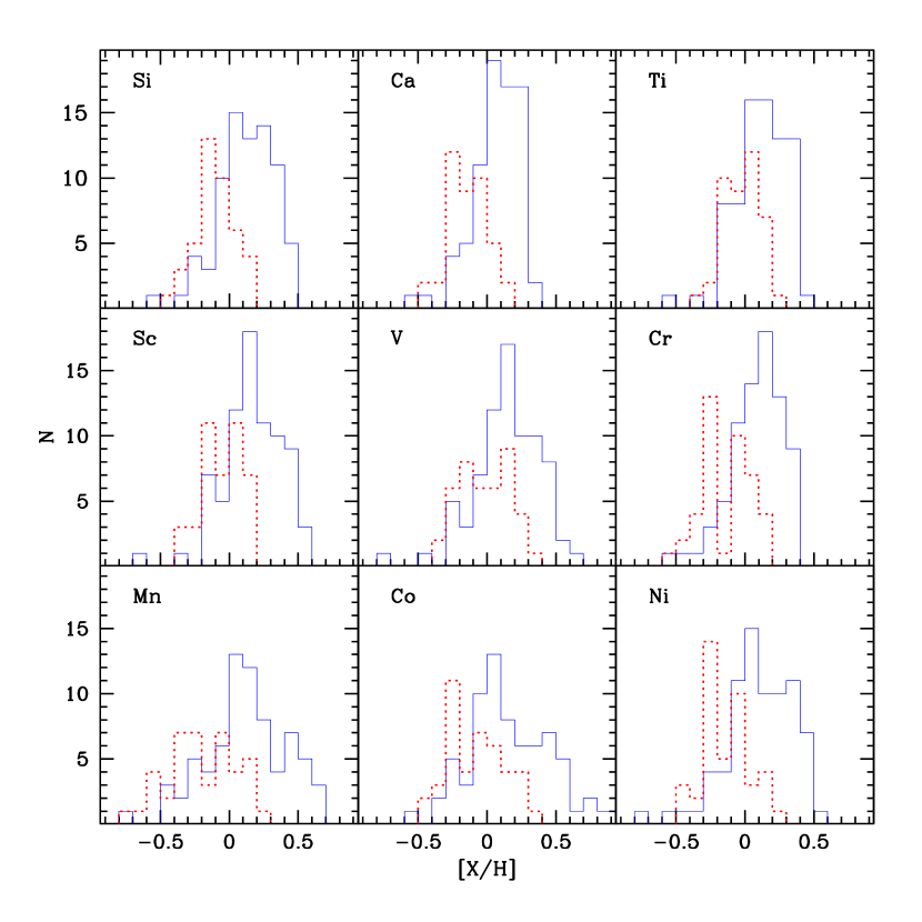
Figure 1: [X/H] distributions of planet-host stars (solid lines) and for our comparison sample (dotted lines).

On the other hand, for a few elements (e.g. Co, and Mn), the star-with-planet distributions appear to be slightly bimodal. The significance and possible implications of this are not clear. It is difficult to conceive that some of the planet hosts had been enriched only in these particular elements (producing the bimodal distributions). If stellar “pollution” were involved, we would not expect large differences between all the elements studied here since their condensation temperatures are not very different (Wasson 1985). This feature may be related to the lack of stars in our samples with [Fe/H] around $+$0.3.

Table 7: Average abundance values $<$[X/H]$>$ for stars with planets and for our comparison sample. Also listed are the rms around the mean and the difference between the two samples for each element. The number of stars is 77 and 42 for the two samples mentioned, respectively.

	Comparison sample		Planet hosts
Species	$<$[X/H]$>$	rms	$<$[X/H]$>$	rms	Difference
Si	$-0.10$	0.15	0.11	0.20	0.21
Ca	$-0.13$	0.14	0.07	0.17	0.20
Ti	$-0.01$	0.13	0.12	0.18	0.13
Sc	$-0.04$	0.15	0.17	0.21	0.21
V	$-0.01$	0.18	0.14	0.24	0.15
Cr	$-0.14$	0.18	0.07	0.22	0.21
Mn	$-0.20$	0.25	0.10	0.33	0.30
Co	$-0.08$	0.20	0.14	0.31	0.22
Ni	$-0.14$	0.18	0.10	0.24	0.24

In Table 7, we list the average values of [X/H] for each element in the two distributions, as well as the rms dispersions and the difference between the average [X/H] for stars with and without planetary-mass companions. The differences vary from 0.13 (for Ti) to 0.30 (for Mn). Given the usually high dispersions around the mean values, these discrepancies are not very significant. In any case, they probably reflect the “normal” chemical evolution of the galaxy (see Sect.4).

3.2 Comparing in the [X/Fe] vs. [Fe/H] plane

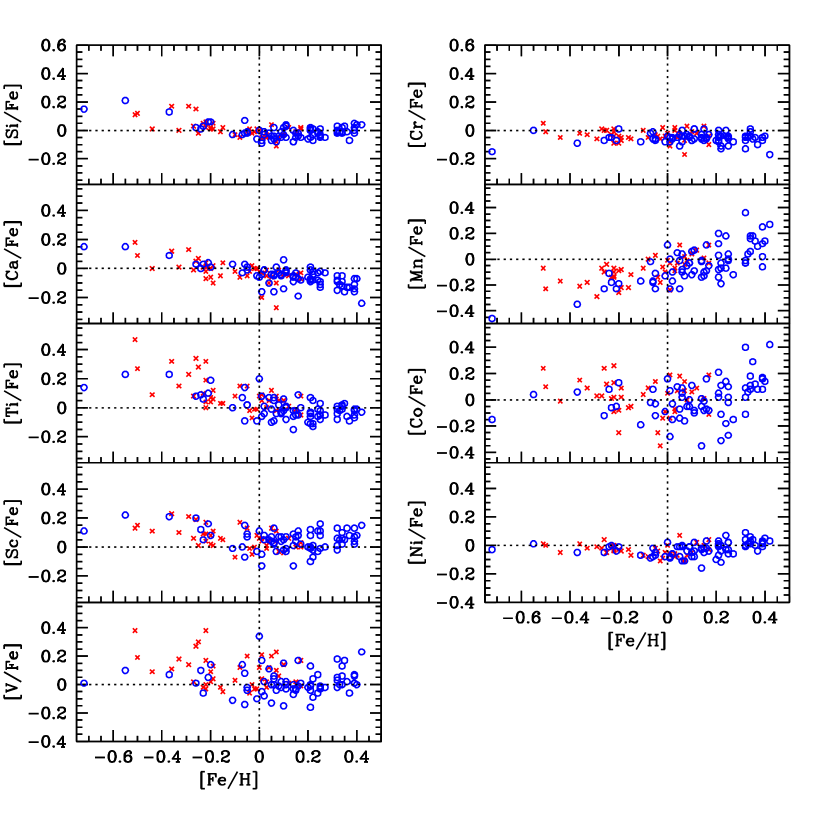
Figure 2: [X/Fe] vs. [Fe/H] plots for the 9 elements studied in this paper. The crosses represent the comparison-sample stars, while the open circles denote the planet-host stars. The dotted lines represent the position of the Sun.

Fig. 2 presents the abundance ratios [X/Fe] of all elements as functions of [Fe/H] for both samples discussed above. Overall, the abundance trends for the stars with planets are nearly indistinguishable from those of the field stars. The only conspicuous difference is the higher average iron content of the planet-host sample. The abundance distributions of stars with giant planets are high [Fe/H] extensions to the curves traced by the field dwarfs without planets (no discontinuity is seen), and in the regions of overlap, we do not find any clearly significant difference between samples.

In Fig. 3, we present the same kind of plots, but with binned average values. For both samples, the bins are centered at [Fe/H]=$-$0.4, $-$0.2, 0.0, 0.2, and 0.4 dex, and are 0.2 dex wide. These plots show that for most elements, the two groups of stars seem to behave in the same manner. Overall, V and Mn, and to a lesser extent Ti and Co, are alone in featuring somewhat distinguishing and systematic traits between the two samples. Field stars are consistently more abundant in vanadium than the planet hosts (up to 0.15 dex apart). Sadakane et al. (2002) proposed a similar overabundance for [Fe/H]$\geq$0.0 dex, except that in their case, the planet-bearing stars were the ones that were vanadium-enriched. Strong star-to-star scatter per metallicity obscures vanadium trends and could be responsible for disagreements between the two groups (see also discussion in the next section). The same is true for Co. Manganese is somewhat more prevalent in the field sample but the fact that a maximum of three spectral lines are available casts some doubt on this assessment. As for Ti, the differences found are small.

All these trends might be related to the NLTE effects described in the Appendix. In any case, these dissimilarities are subtle, and may very well be negligible, but they are still intriguing enough to merit renewed tests using comparable techniques and parameters.

It is important to note that these possible differences, if confirmed, are probably not indicators of differential accretion of material by the star, for example, since the condensation temperatures of these elements are all in a short range of merely $\sim$300 K (e.g. Wasson 1985) (they are all refractory). The reason would then probably have to do with the source of the metals examined. Whether the general trends (see discussion in Sect.4) are so that planets might form more easily around stars with specific metallicity ratios is not excluded. Once again, this does not seem very likely given the nature of the elements analyzed here.

Unfortunately, this comparison is somewhat limited since the two stellar samples overlap in a small region of [Fe/H]. In particular, the (high-)metallicity region where most of the planet hosts are located does not contain many comparison stars. Thus, we can not completely exclude the existence of important differences for these objects.

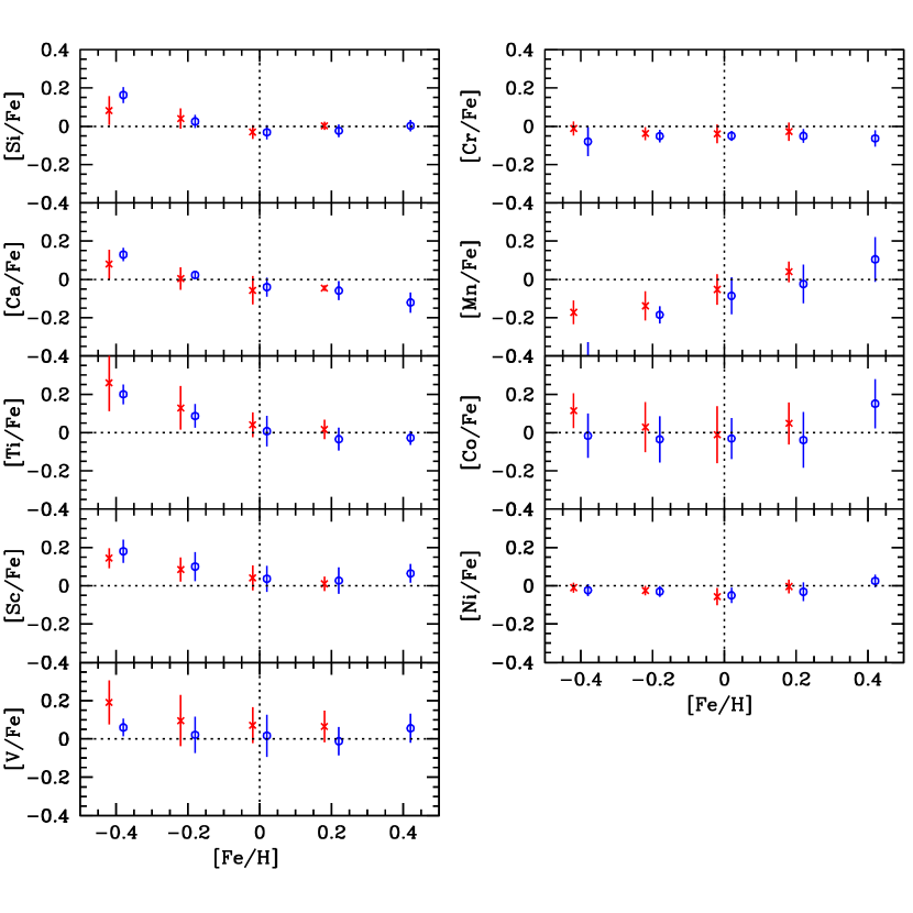
Figure 3: Same as Fig. 2, but now using binned average values. For both samples the bins are centered at [Fe/H]=$-$0.4, $-$0.2, 0.0, 0.2, and 0.4 dex, and are 0.2 dex wide. The crosses represent the comparison-sample stars, while the circles denote the planet-host stars. The error bars depict the rms around the mean value.

4 Galactic trends

Although the main goal of this work is to compare the elemental distributions for stars with and without giant-planetary companions, a clear byproduct of this study is the chance to increase our knowledge of galactic chemical evolution trends. This is especially true for the high [Fe/H] region, for which the number of detailed studies is still limited.

In this section, we will therefore make a brief comparison of the results we have obtained with those presented in the major studies in the literature regarding this subject. Given the small (and probably insignificant) differences argued above between planet hosts and non-hosts, we will consider our sample as a whole in the rest of the analysis. We will also keep the discussion brief, leaving the interpretation of the galactic chemical evolution to a future paper.

Of course, some of the trends discussed below (in particular for the more metal-rich stars) may eventually be seen as signatures of the presence of planets, since these stars are (in our sample) all planet hosts. For example, differences between the observed trends and those published in the literature could reflect the presence of planets, and would thus be of great importance. However, the trends are probably (and easily) best interpreted as simple byproducts of galactic evolution, and their relation to the presence of a planet are probably coincidental (besides the fact, of course, that these are the more globally metal-rich stars). Furthermore, given that there are no metal-rich stars that lack planets in the current sample, it is not possible to compare the two groups of stars in these high-[Fe/H] regions of the plots. Again, this means that we cannot exclude that the observed trends for the high-[Fe/H] stars are due to some kind of planetary induced chemical variation, or that the abundance ratios for these stars are themselves influencing the efficiency of planetary formation.

4.1 Silicon

From Figs. 2 and 3, we can see that [Si/Fe] is inversely related to [Fe/H] for $-$0.6$<$[Fe/H]$<$$-$0.2 dex, and then appears to level off at $-$0.2$<$[Fe/H]$<$0.0 dex. Similar results were also found by Edvardsson et al. (1993) (hereafter EAGLNT) and Chen et al. (2000) (hereafter, C00). As these authors have found, the dispersion in the abundance ratio [Si/Fe] is very small in the metallicity range studied here.

For metallicities above solar, our data shows a plateau in the [Si/Fe] vs. [Fe/H] relation. Again, this result is compatible with the one found by both EAGLNT and C00. However, we also see a hint of an increase in the [Si/Fe] vs. [Fe/H] trend for [Fe/H]$>$0.3 (and maybe before this value). This upturn was already slightly noticeable in the data of EAGLNT, but given the low upper limit in [Fe/H] of the objects analyzed by these authors, no serious conclusion was possible. Feltzing & Gustafsson (1998) (hereafter FG98) analyzed stars with [Fe/H] up to $\sim$0.4 dex, but they found a much larger scatter in the abundances; their results do not permit an investigation of the behavior of [Si/Fe] for these high metallicities. We note, however, that the data for planet-host stars of Gonzalez et al. (2001) (see their Fig. 10) does not support the presence of such a trend.

4.2 Calcium

For [Fe/H] lower than solar, the behavior of [Ca/Fe] is very similar to the one described above for Si. Contrary to this latter element, the [Ca/Fe] ratio seems to decrease almost continuously for the entire metallicity range studied in this paper (see Figs. 2 and 3). A glance at the figures suggests the presence of a plateau in the region $-$0.2$<$[Fe/H]$<$0.2 dex, immediately followed, for higher metallicities, by a clear drop-off. While the former trends have been found both by FG98 and EAGLNT (also visible in the plots of Sadakane et al. (2002)), this latter downturn was not clearly visible in the data presented by these authors, probably because their data never ventured above $\sim$0.4 and 0.3 dex, respectively. This downturn was also seen in the data of Gonzalez et al. (2001).

Once again, the dispersion of our abundance is very small (except for abundances around [Fe/H]=0.0-0.2 dex for which a few stragglers are present: HD 209100 with [Ca/Fe]=$-$0.20 and HD 216803 with [Ca/Fe]=$-$0.27 dex, both very cool dwarfs). This fact gives us confidence for the reliability of the trends discussed above. The scatter for these two objects was first explained by the existence of NLTE effects (see discussion in FG98). However, Thoren (2000) has shown that this was not the main reason for the observed discrepancy. Furthermore, Thoren & Feltzing (2000) demonstrated that the use of temperatures computed from a strict excitation equilibrium (as used here) eliminates most NLTE effects. As also discussed in the Appendix, there still seems to be a systematic decline of the [Ca/Fe] abundance ratios with decreasing temperature for the most metal-rich stars. We note, though, that this effect cannot be responsible for the downturn of [Ca/Fe] seen for the higher [Fe/H] stars since the stars that occupy this region of the plot ([Fe/H]$>$0) present all kinds of effective temperatures.

4.3 Titanium

Established by FG98, EAGLNT, and C00, [Ti/Fe] seems to follow a continuous decline with [Fe/H]. The [Ti/Fe] distribution has a more precipitous slope than for [Si/Fe] and [Ca/Fe], but it also carries a wider dispersion (see Fig. 2). Judging from Figs. 2 and 3, titanium drops until $-0.2<[$Fe$/$H$]<0.0$ dex and then settles. This supports C00 and is unlike the continuing downward trend proposed by EAGLNT.

The results of FG98, C00, EAGLNT, and Gonzalez et al. (2001) have all reproduced the pronounced scatter in titanium abundances seen here. The scatter can probably be attributed to NLTE effects over things like line-blending or real “physical” galactic evolution effects. As mentioned in the Appendix, there is a large dependence of the [Ti/Fe] as a function of T_eff, which is likely behind the large scatter. Given that the stars with [Fe/H] below $-$0.2 are, in average, cooler (by about 200 K) than the rest of the sample, it is possible that part (but very unlikely all) of the decreasing trend discussed above is due to NLTE effects..

4.4 Scandium

Scandium abundances begin above solar (about 0.15 dex) at the iron-poor end of the distributions and then settle at [Fe/H]$\sim$$-$0.2 dex. The distribution of scandium graphed in Fig. 2 basically mimics the trends of the $\alpha$-elements (in particular Si). The figures also show that there might be a slight upswing in scandium concentrations for iron-rich stars, much like the upturn that potentially characterizes the [Si/Fe] ratio.

Nissen et al. (2000) offered a thorough study of the abundances of scandium. The results presented here for the metallicity range up to [Fe/H]$\sim$0.0 support their trends. Their study stops at solar metallicities, and does not permit the confirmation of our interesting result for the more metal-rich stars. It is interesting to note, however, that in the [Sc/Fe] vs. [Fe/H] plot presented by Sadakane et al. (2002) (combining their data with those of C00 and FG98) the same upward trend is suggested.

4.5 Vanadium

Despite the large scatter, the overall shape of the vanadium distribution resembles the functions for silicon and scandium: overabundance at the iron-poor end, (almost) flat at solar values, and a potential (but not clear) upturn for the most iron-rich stars. An overabundance of vanadium ($[$V$/$Fe$]\sim 0.2$ dex for iron-poor stars) was not detected by either FG98 or C00 (although the latter’s plots hint at some trend), who proposed instead that the $[$V$/$Fe$]$ ratio followed iron for all metallicities. However, a look at Fig. 19 of FG98 suggests a slight upper trend for higher metallicities as observed here.

It is important to note that vanadium seems to suffer strongly from NLTE effects (see Appendix). For all metallicities, our analysis gives a decreasing [V/Fe] with increasing effective temperature trend. This is probably the reason for the large scatter seen in Fig. 2. As discussed for Ti, NLTE effects might e.g. be responsible (in part) for the decreasing trend seen for lower metallicity stars (Fe/H]$<$$-$0.2).

4.6 Chromium

Figs. 2 and 3 illustrate that the $[$Cr$/$Fe$]$ ratio stays fairly constant with increasing $[$Fe$/$H$]$, as was found by FG98 and C00. For a given metallicity, chromium abundances have about half the star-to-star scatter encountered by C00. The authors noted that with a few weak lines at their disposal, any dependence relation was tentative, and that the source of the scatter in $[$Cr$/$Fe$]$ could not be readily ascribed to either systematic errors or cosmic effects. The C00 chromium distribution flirted with solar values whereas the stars in the current survey have about 0.05 dex less chromium than the Sun. Although this shift is close to the established error, it might conceal an underestimation if we suppose that the abundances of solar-type stars should reflect solar values. Nevertheless, even if this indicates a systematic error, the trends discussed should not be affected. As noted by FG98, the flatness is well explained by the balance between the different types of sources for Fe and Cr (Timmes et al. 1995).

4.7 Manganese

Manganese abundances increase with iron for the metallicity range studied, in agreement with Nissen et al. (2000), FG98, and Sadakane et al. (2002). Figs. 2 and 3 show that $[$Mn$/$Fe$]$ begins with an underabundance of about $-0.2$ dex at [Fe/H]$\sim$$-$0.4, then rises to solar levels and beyond for the higher-metallicity stars in our sample.

4.8 Cobalt

Hampered by a low number of measurable lines and possible strong NLTE effects (see Appendix), cobalt abundances possess substantial star-to-star scatter, but the distribution appears to veer upwards for iron-rich stars, a result similar to the one found by both FG98 and Sadakane et al. (2002) (a trend that recalls those of Si, Sc, and V in our analysis). Given the dispersion in our data, we cannot confirm the long plateau found by the former authors for [Fe/H] below solar. But our data insinuates decreasing [Co/Fe] as a function of [Fe/H] up to metallicities around solar (which, as for Ti and V, might in part be due to NLTE effects).

4.9 Nickel

Echoing the results of FG98 and C00, nickel abundances follow iron with low interstellar scatter per metallicity (Fig. 2). The shape of the $[$Ni$/$Fe$]$ distribution exhibits a slight decreasing trend (but probably a plateau) for $-0.6<[$Fe$/$H$]<0.0$ dex, and then an upturn. This upturn was also visible in the data of FG98, and was discussed by C00. Furthermore, EAGLNT showed that their constant trend of $[$Ni$/$Fe$]=0.0$ became disrupted and overabundance ensued once the stars passed the solar metallicity.

It should be noted that the nickel abundances derived here are somewhat lower than the values offered by the other authors. The reason for this might have to do with the determination of the $\log{gf}$ values. However, as already noted above, the general trends should not perish from any systematic errors. A similar result might indeed be found in the study of FG98.

5 Concluding Remarks

In this paper, we have derived precise and uniform abundances for nine different elements (other than iron) for a large sample of planet-host stars, as well as in a comparison sample of stars without any discovered planetary-mass companions. The results were used to compare the two samples and to look for possible differences eventually connected to the presence of planets. The data was also used to explore galactic chemical evolution trends.

Overall, we found that no significant differences were present between stars with and without planetary companions, at least in the metallicity region where the two samples overlap. The only elements showing potential trends were V, Mn, and to a lesser extent Ti and Co. However, in no case were the differences clear. These might be related e.g. to NLTE effects – see Appendix A.

Furthermore, the available data gave us the possibility to investigate galactic chemical evolution trends for metal-rich stars with unprecedented detail. The results revealed some interesting (and previously unnoticed) behavior concerning the metal-rich tail of the distributions (particularly for Si, Ca, and possibly Sc, and V).

The study of metal abundances in planet-host stars has already helped to clarify the formation processes of giant planets. For example, they have shown that the efficiency of planetary formation is a strong function of the metallicity (e.g. Santos et al. 2001). More details are likely to emerge as new planets are found. The continuing study of the abundances in planet hosts might indeed be a source of many more compelling results. The determination of the abundances of volatile elements, for example, will give us the chance to discuss the relative importance of differential accretion (e.g. Gonzalez 1997; Smith et al. 2001; Sadakane et al. 2002) in planet-host stars. Further interesting results might be derived from the study of specific elemental abundance ratios like [C/O] (e.g. Gaidos 2000). On the other hand, some clues might come from the study of the sources of the elements present in planet-harboring stars. At present, we are working to extend the current study to other elements, as well as to increase the number of stars in the current samples. Soon we hope to be able to answer many of the questions that were raised here.

Appendix A Possible NLTE effects

In this article, all the elemental abundances are derived assuming LTE. However, the dominance of this regime is questionable in solar atmospheres. The assumption of LTE and a plane-parallel, homogeneous model atmosphere can introduce systematic errors, and change the slope of elemental abundance ratios $[$X$/$H$]$ versus $[$Fe$/$H$]$ (e.g. Edvardsson et al. 1993). Plane-parallel atmospheres can lead to too little adiabatic cooling and too much radiative heating (e.g. Chen et al. 2000).

If, for metal-poor stars, the NLTE effects have been shown to be important (e.g. Edvardsson et al. 1993), they are usually not very strong for their metal-rich counterparts (Edvardsson et al. 1993), and NLTE corrections are frequently of the same order of magnitude (or lower) as the errors in the analysis. Thévenin & Idiart (1999) have shown, for example, that the NLTE effects on iron abundances for metal-rich dwarfs are very small.

However, and at least for a few elements, the NLTE corrections seem to be quite strong. For example, Feltzing & Gustafsson (1998) noticed that cool, metal-rich stars show up as underabundant in calcium, an effect attributed to NLTE effects, as previously discussed in Drake (1991). In this case, at least part of the errors were later shown to be due to wrongly-calculated damping parameters (Thoren 2000). But similar behavior was found by Feltzing & Gustafsson (1998) for nickel, and other elements studied by these authors also showed odd abundances.

In a recent paper, Thoren & Feltzing (2000) showed that the use of a strict excitation equilibrium eliminates (at least in part) this problem. Following this result, and since this is the method that we have used to estimate the effective temperatures for our program stars in Santos et al. (2000, 2001, 2003), we should expect our parameters to be reasonably free from NLTE effects (i.e. NLTE corrections should not be very strong).

In Fig.4, we plot the abundance ratios [X/Fe] for the nine elements studied in this paper against T_eff. In these plots, the stars are separated into two groups of metallicity: objects with [Fe/H] lower than solar (circles) and above solar (disks). For each group, a least-squares fit was done. The slopes are listed in Table 8.

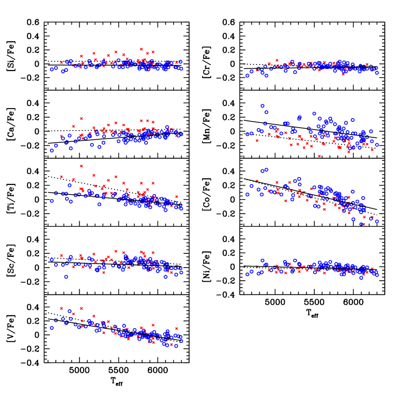
Figure 4: [X/Fe] vs. T_eff plots for the nine elements studied in this paper. The stars are separated based on their metallicities. The slopes represent linear least-squares fits to the iron-poor stars (crosses and dashed lines) and the iron-rich stars (circles and solid lines).

Table 8: Slopes of $[$X$/$Fe$]$ ratios as functions of effective temperatures in dex per 1000 K.

Species	slope: $[$Fe$/$H$]<0$	slope: $[$Fe$/$H$]\geq 0$
Si	$-0.001\pm 0.028$	$-0.001\pm 0.011$
Ca	$0.006\pm 0.026$	$0.083\pm 0.014$
Ti	$-0.213\pm 0.041$	$-0.093\pm 0.012$
Sc	$-0.050\pm 0.032$	$-0.031\pm 0.016$
V	$-0.246\pm 0.034$	$-0.176\pm 0.014$
Cr	$-0.034\pm 0.013$	$0.013\pm 0.013$
Mn	$-0.107\pm 0.030$	$-0.152\pm 0.033$
Co	$-0.294\pm 0.033$	$-0.243\pm 0.033$
Ni	$-0.024\pm 0.013$	$-0.025\pm 0.015$

As we can see from these plots, a few elements have considerable dependence of the derived abundances on the effective temperature. If for Si, Sc, Cr, Ni, and Ca the effects seem to be very small, for V, Ti and Co the difference between the K and F-dwarfs in our sample are of the order of 0.2 to 0.3 dex. The situation for Mn is intermediate. Furthermore, for a few species we find relevant distinctions between the slopes for iron-rich and iron-poor stars, namely for Ca and Ti. For the former of these two elements, only the metal-rich dwarfs seem to be affected by a dependence on T_eff, whereas for Ti, the effect seems to be much stronger for the most metal-poor objects. We note that the sensitivity of the Ti I lines to NLTE effects has already been discussed (e.g. Brown et al. 1983). A test with Ti ii lines has shown that the abundances obtained from these present a much smaller dispersion; the use of Ti ii might indeed be preferable (Shchukina 2002, personal communication). In fact, since Ti ii abundances are barely sensitive to T_eff (Santos et al. 2000), it is normal that no relation between [Ti ii/Fe] and temperature is present.

The trends observed for V, Ti, Co, and Mn are reasons behind the large dispersions observed in the plots of Fig. 2. We note that for most of the remaining elements the scatter is very small (except perhaps for Sc, for which the cause may lie in the low number of spectral lines used).

Although we do not pretend to explain the causes for the observed trends here, it is important to note them for future studies. In particular, for the elements that seem to suffer more from these kind of effects, a precise and reliable comparison between planetary hosts and non-host probably needs the use of NLTE analysis.