Abstract

The Sloan Digital Sky Survey (SDSS) is collecting photometry and intermediate resolution spectra for $\sim 10^{5}$ stars in the thick-disk and stellar halo of the Milky Way. This massive dataset can be used to infer the properties of the stars that make up these structures, and considerably deepen our vision of the old components of the Galaxy. We devise tools for automatic analysis of the SDSS photometric and spectroscopic data based on plane-parallel line-blanketed LTE model atmospheres and fast optimization algorithms. A preliminary study of about 5000 stars in the Early Data Release gives a hint of the vast amount of information that the SDSS stellar sample contains.

Chapter 0 New Resources to Explore the
Old Galaxy: Mining the SDSS

1 Introduction

The Sloan Digital Sky Survey is an ambitious project that is imaging about one fourth of the sky with five broad-band filters. The survey includes followup intermediate-dispersion ($\lambda/\delta\lambda\simeq 1800$) spectroscopy (York et al. 2000). The final catalog is expected to include photometry and spectroscopy for about $10^{8}$ and $10^{6}$ sources, respectively. Focused on extragalactic science, the spectroscopic survey aims at amassing the largest possible collection of galaxy redshifts. The dedicated f/5 Ritchey-Chrétien-like 2.5m telescope has a three-degree field of view. In the spectroscopic mode, up to 640 (180$\mu$m or 3 arcsec Ø) fibers can be simultaneously positioned on the focal plane to feed two identical spectrographs. Each spectrograph has a blue and a red arm that provide continuous coverage in the range 381–910 nm.

The selection criteria for the spectroscopic targets are rather complex (Eisenstein et al. 2001; Richards et al. 2002; Stoughton et al. 2002; Strauss et al. 2002). Galaxies and quasar candidates take about 90% of the fibers, with the remaining used to observe the sky background and Galactic stars, which are either selected for being peculiar (brown dwarfs, blue-horizontal branch stars, carbon stars, etc.), or intended for reddening and flux calibration. In addition, almost a third of the quasar candidates in the Early Data Release turned out to be stars. Nearly $\sim 10^{5}$ stellar spectra will be released by the end of the survey in 2006. With exposure times per plate of the order of 45 minutes, the targeted stars have $V$ magnitudes in the range 14–21, signal-to-noise ratios ($S/N$) between 5 and 150, and lie at distances of up to hundreds of kiloparsecs from the Galactic plane. When released, the SDSS stellar spectra will constitute the largest spectroscopic survey of the Galactic thick-disk and halo populations yet assembled.

2 Analysis

The analysis of a massive dataset calls for automated procedures. The SDSS images and spectra are processed by a series of pipelines specialized in tasks such as astrometric, wavelength, and flux calibrations, aperture photometry, or the extraction and classification of spectra. Starting from the released photometry and spectra for Galactic stars, we are interested in a detailed classification based on the fundamental atmospheric parameters. Projected radial velocities are directly measurable from the spectra. Given the large spectral coverage, we expect to be able to quantify the interstellar reddening towards the observed stars. Stellar metallicities, and even perhaps the abundance ratios of chemical elements or groups of elements well-represented in the spectra, are obviously some of the most valuable information to search for. It is also most interesting to use the derived stellar parameters, chemical abundances, and interstellar reddening to infer distances and ages.

We make use of the SDSS ($ugriz$) photometry and the $\sim 3800$ pixels in an object’s spectrum altogether. We found it helpful to trade resolution for $S/N$, and therefore the spectra are smoothed to $\lambda/\delta\lambda=1000$ by convolution with a Gaussian profile. As absolute fluxes are not relevant at this point, we use photometric indices and normalize the spectra $\{S_{i}\}$ to satisfy $\sum_{i=1}^{m}S_{i}/m=0.5$. The relevant data vector is ${\bf T}\equiv\{u-g,g-r,r-i,i-z,S_{1},S_{2},S_{3},\dots,S_{m}\}$, where $m=2600$. We model T with plane-parallel line-blanketed LTE model atmospheres and radiative transfer calculations, as a function of the stellar parameters (effective temperature $T_{\rm eff}$, surface gravity $g$, and overall metallicity [Fe/H]). The collection of model atmospheres and low-resolution synthetic spectra of Kurucz (1993) is used. This grid was calculated with a mixing-length $l/H_{p}=1.25$, and a micro-turbulence of 2 km s^-1. The low-dispersion spectra are convolved with the SDSS filter responses (Strauss & Gunn 2001). The atmospheric structures are used to produce LTE synthetic spectra with a resolving power $\lambda/\delta\lambda=1000$ between 381 and 910 nm. Balmer line profiles are treated as in Hubeny, Hummer, & Lanz (1994). The radiative transfer equation is solved with the code synspec (Hubeny & Lanz 2000), using very simple continuous opacities: H, H^-, Rayleigh and electron scattering (with the prescriptions in Hubeny 1988). The calculations included 131821 atomic line transitions, but no molecular features.

Both photometric magnitudes and spectra are computed for a discreet $12\times 4\times 6$ grid spanning the ranges 4500 to 10000 K, 2.0 to 5.0 dex, and $-4.5$ to $+0.5$ dex in $T_{\rm eff}$, $\log g$ (c.g.s units), and [Fe/H], respectively. The interstellar reddening ($E(B-V)$) is parameterized as in Fitzpatrick (1999), adopting $R\equiv A(V)/E(B-V)=3.1$. This parameter gives one more dimension to the grid. We consider $E(B-V)$ in the range $0.0-0.1$ with just three values. Model spectra and photometry for sets of parameters off the grid nodes are derived by multi-linear interpolation.

Some elements show abundance ratios to iron that are non-solar in metal-poor stars. This is largely ignored in our modeling. However, we consider enhancements to the abundances of Mg and Ca in metal-poor stars when calculating synthetic spectra because these elements produce strong lines on which our analysis heavily relies. Following Beers et al. (1999) we adopt [$\alpha$/Fe] $\simeq$ [Ca/Fe] $\simeq$ [Mg/Fe]:

$$[\alpha/Fe]=\left\{\begin{tabular}[]{cc}0&if $0\geq$ [Fe/H]\\ $-0.267$ [Fe/H]&if $-1.5\leq$ [Fe/H] $<0$\\ $+0.4$&if [Fe/H] $<-1.5$.\\ \end{tabular}\right.$$ (1)

We perform a search for the model parameters that minimize the distance between the model T ($T_{\rm eff},g$, [Fe/H], $E(B-V)$) and the observations’ vector O. In a $\chi^{2}$ fashion, we define such distance as

$$\mu=\sum_{i=1}^{m+4}{W_{i}(O_{i}-T_{i})^{2}}$$ (2)

where the weights $W_{i}$ are optimized for performance. The search is accomplished by using either the Nelder-Mead simplex method (Nelder & Mead 1965) or a genetic algorithm (Carroll 1999). The multi-linear interpolation was deemed as accurate enough after repeating the interpolations with the decimal logarithm of the fluxes. Testing with finer grids in $\log g$, [Fe/H], and $E(B-V)$, led only to marginal variations in the results. Classification of a single spectrum takes a few seconds on a 600 MHz workstation.

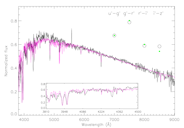
Figure 1: Comparison of observed spectra (black line) and photometric indices (open circles) with the best-fitting model (red line and green circles) for one of the EDR stars. The inset shows an enlarge view of the bluest part of the spectrum. The primes in the photometric magnitudes are related to technical subtleties between different calibrations. For our purposes these are the same as the non-primed magnitudes we refer to in the text.

Fig. 1 shows an example of observed (black) and model (red and green) fluxes for one of the EDR stars that we fit with $T_{\rm eff}=5388$ K, $\log g=4.71$, [Fe/H]$=-1.2$, and $E(B-V)=0.004$. The inset plot gives an expanded view of the blue part of the spectrum. Note that molecular features, such as the G band (CH) at $\sim 4300$ Å are not reproduced by the model spectrum. The photometric indices have been scaled to fit in the graph’s box and placed at arbitrary wavelengths.

Once the atmospheric parameters are defined, we make use of stellar evolutionary calculations by the Padova group (Alongi et al. 1993; Bressan et al. 1993; Fagotto et al. 1994; Bertelli et al. 1994) to find the best estimates for other stellar parameters: radius, $M_{V}$, mass ($M$), $Age$, etc. With the atmospheric parameters and their uncertainties in hand we define a normalized probability density distribution that is Normal for $T_{\rm eff}$ and $\log g$, and a boxcar function in $\log(Z/Z_{\odot})$

$$P\propto\exp\left[-\left(\frac{T_{\rm eff}-T_{\rm eff}^{*}}{\sqrt{2}\sigma(T_{\rm eff})}\right)^{2}\right]\exp\left[-\left(\frac{\log g-\log g^{*}}{\sqrt{2}\sigma(\log g)}\right)^{2}\right]B\left(\log(Z/Z_{\odot})\right),$$ (3)

which is then used to find the best estimate of a stellar parameter $X$ by integration over the space ($Z/H$, Age, and initial mass $M$) that characterizes the stellar isochrones of Bertelli et al. (1994)

$$\bar{X}=\int_{Z/H}\int_{Age}\int_{M}XP(Z/H,Age,M)d(Z/Z_{\odot})d(Age)dM.$$ (4)

The isochrones employed do not consider enhancements in the abundances of the $\alpha$ elements for metal-poor stars. Thus, we simply equate [Fe/H] $=\log(Z/Z_{\odot})$. More realistic relations should take this into account, and will be explored in the future.

Finally, the magnitudes in the SDSS passbands can be used to estimate the Johnson $V$ magnitudes of the stars (Zhao & Newberg 2002). Knowing $M_{V}$ and the reddening, it is then straightforward to derive distances.

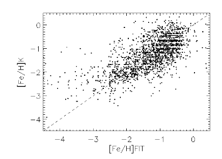
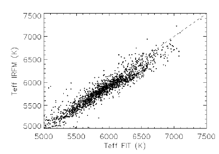
Figure 2: Top panel: Comparison between the [Fe/H] derived by our spectral fitting technique and those with the K method of Beers et al. (1999). Lower panel: The effective temperatures from fitting the spectra are compared to those based on the photometry and the IRFM calibrations of Alonso et al. (1996, 1999). The dashed lines have a slope of one.

3 Checking on $T_{\rm eff}$ and [Fe/H]

The inclusion of the Ca K line and the seven first members of the Balmer series in the EDR spectra makes them suitable for the application of well-tested techniques developed for the followup of stars in the HK survey (Beers, Preston & Shectman 1992; Beers et al. 1990; Beers et al. 1999).

After measuring the pseudo-equivalent widths of the relevant spectral features and estimating the $(B-V)$ colors from the SDSS photometry, we obtain a second, relatively independent, measure of the metallicities of the EDR stars. After visual inspection, a subsample of 1910 stars was deemed of reasonably good quality, and their metallicities are compared with those determined by spectral fitting in the upper panel of Fig. 2. The overall agreement for [Fe/H] $>-2.5$ is reasonable, with a scatter of about 0.5 dex. A systematic discrepancy is apparent for the most metal-poor stars. This disagreement exceeds the internal uncertainties of each method and should be investigated. We have found that, in the presence of severe noise, the optimization algorithms tend to underestimate the metallicity. We should also note that a spurious feature is apparent in many EDR spectra right between the Ca H and K lines, which might be affecting the Ca II K method.

The $(B-V)$ colors estimated from the SDSS $ugriz$ photometry and the stellar metallicities were fed to the photometric calibrations of Alonso et al. (1996, 1999), which are based on the Infrared Flux Method (IRFM; Blackwell, Shallis & Selby 1979). These calibrations have an internal scatter of about 2% and an uncertainty in the zero point of about 1%. Therefore, they offer a reliable external check to the $T_{\rm eff}$s determined automatically from the simultaneous analysis of EDR spectra and photometry. The interstellar reddening was corrected using the values determined spectroscopically. The lower panel of Fig. 2 shows a pleasing correspondence between the two $T_{\rm eff}$ determinations. The IRFM $T_{\rm eff}$s are, on average, lower by 66 K with an rms scatter between the two scales of 160 K.

4 Application to the EDR. Preliminary results.

The SDSS begun standard operations in April 2000. The Early Data Release (EDR; Stoughton et al. 2002) was made public on June 5, 2001. It consists of 462 square degrees of imaging data and 54008 spectra. The data were acquired in three regions, two of them following the celestial equator in the southern and northern Galactic skies, and a third which overlaps with the SIRTF First Look Survey (Storrie-Lombardi et al. 2001). We have selected the spectra that were finally identified as stellar. Our sample includes 5604 objects, but we were only able to identify Balmer lines in 4714, whose distribution in Galactic coordinates is shown in Fig. 3. The brightness distribution of the sample ranges between $V=$ 14 and 21, and it is depicted in Fig. 4.

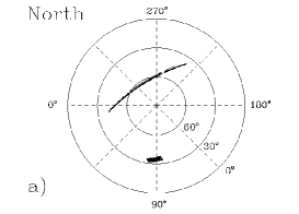
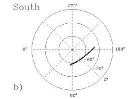
Figure 3: Location of the EDR stars in galactic coordinates for each hemisphere. The galactic latitude corresponds to the radius in the plot and the longitude to the azimuth.

Figure 4: Distribution of brightness for the EDR stars. $V$ magnitudes were not directly measured, but inferred from the SDSS $ugriz$ fluxes following Zhao & Newberg (2002).

It is interesting to compare the distances found for the sample as a function of the stellar $T_{\rm eff}$. In Fig. 5, dwarf stars define a tilted band that marks the minimum distance at a given $T_{\rm eff}$. The K-type dwarfs in the sample are located at distances of 1–2 Kpc. Warmer stars on the main sequence are more distant, with an obvious drop in density at $T_{\rm eff}\simeq 6500$ K. Some areas in Fig. 5 are underpopulated. Subgiants cause the overdensity in a band nearly perpendicular to the main-sequence that crosses it at about $T_{\rm eff}=7400$ K. As stars evolve off the main-sequence, they become cooler but more luminous, and can be seen at larger distances. A second band parallel to the first is weakly apparent intersecting the main-sequence at a $T_{\rm eff}$ of $\sim 6000-6300$ K. Interpreting these features as ’turn-offs’, this diagram marks two preferred ages for the sample.

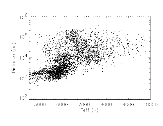
Figure 5: Position of the EDR stars in the $T_{\rm eff}-$ distance plane.

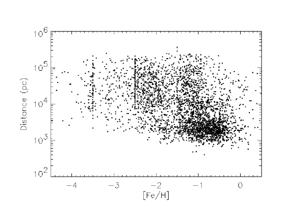
Figure 6: Position of the EDR stars in the [Fe/H] – distance plane.

The limiting magnitude for the sample of EDR stellar spectra is $V\simeq 20-21$. G-type giant stars with $M_{V}\sim 1$ allow us to reach out to distances as far as $\sim 50$ Kpc, but supergiants with $M_{V}\sim-4$ extend our scope about ten times farther. The sharp drop in density of stars for distances larger than about 200 Kpc may or may not be a selection effect.

Another interesting projection of the data is on the plane [Fe/H] vs. distance (see Fig. 6). The most metal-poor stars ([Fe/H]$<-3$) appear only at distances larger than 3 Kpc. It is apparent in the Figure that many stars clump at small distances ($\leq 4$ Kpc) in the metallicity range $-1.2<$[Fe/H]$<-0.4$. It is very tempting to identify this population with the thick disk (see, e.g., Gilmore & Reid 1983; Reddy et al. 2003). The concentration of stars at exactly the grid nodes in [Fe/H] ($-3.5,-2.5,\dots$) is an artifact of the search algorithm that we do not understand yet.

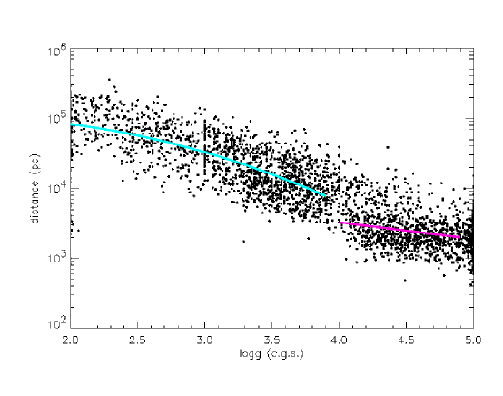
Figure 7: The graph shows which stars cover which range of distances. Two components have been fitted by least-squares to the data. These can be associated with the halo (blue), and thick disk (red; but also contaminated with halo stars).

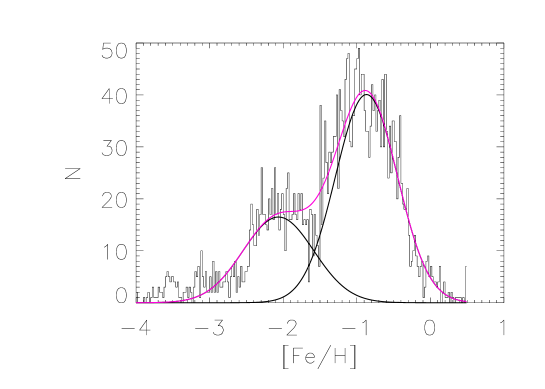
Figure 8: Histograms of the number of stars analyzed in the EDR sample as a function of distance (upper panel) and [Fe/H] (lower). In the lower panel, a two-Gaussian model has been fitted (red) curve. The individual components of the model are also shown in black.

Fig. 7 shows the range of distances that each luminosity class covers. In this Figure, the thick disk and halo populations are clearly separated. The thick disk stars show a density distribution that rapidly falls beyond 2 Kpc. The halo star counts, however, decline slowly with distance. Our next challenge is correcting the involved selection effects to study the true density law of the halo.

The distribution of stars in Fig. 6 can be collapsed on one axis at a time, as shown in Fig. 8. In the upper panel, the clump of stars that we identify with the thick disk becomes even more obvious. The distribution of brightness for the EDR stars peaks at $V\sim 18$ mag, which corresponds to distances of $\sim 10^{4.4}$ pc for giants and $\sim 10^{5.4}$ pc for supergiants. The continuous shape of the number density of stars between $10^{4}$ and $10^{5.5}$ pc strongly suggests that the observed density decline is mainly driven by the reality in the Galactic stellar halo.

K, G, and F-type dwarfs in the EDR allow us to cover the range $\sim 10^{3}-10^{4}$ pc, and therefore they essentially are the thick disk population in our sample (see Fig. 1.6). Nearby giants and supergiants brighter than $V\sim 14$ mag are rejected by the selection algorithm to avoid saturating the detector. They can only cover distances larger than $10^{3.6}$ pc. Together, these selection effects provide a simple explanation for the decrease in number density of stars at $10^{3.7-3.8}$ pc. In fact, the star counts at $10^{3.5}$ pc seem to recover the trend apparent at distances larger than 10 Kpc.

The lower panel of Fig. 8 reveals that the metallicity distribution can be approximately modeled with only two Gaussian components. A first component, or thick-disk, centered at [Fe/H] $=-0.9$ ($\sigma=0.4)$ dex, and a second-component, or stellar halo, centered at [Fe/H] $=-2.1$ ($\sigma=0.5$) dex. With the selected bin size (0.02 dex), the artificial overdensities at the grid nodes are easy to spot and have been excluded from this figure.

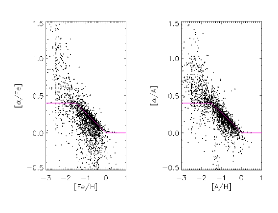
Figure 9: In an attempt to estimate the abundance ratio between the $\alpha$ elements (Mg and Ca) and Fe, we vary the weights in our fitting procedure to favor some lines over others as metallicity indicators. When all lines are considered we derive [A/H], and when bias the analysis for, and against, lines of Mg and Ca, we obtain [$\alpha$/H] and [Fe/H], respectively. The red line corresponds to the assumption adopted for calculating the synthetic spectra, as given in Eq. 1.

The weights $W_{i}$ in Eq. 2 are about 500 times larger for any of the SDSS photometric indices than for any given pixel in the spectra. The weights for the spectra are heavily biased towards lines, which carry most of the information on the parameters we are interested in. The relevant lines in the optical spectrum of a metal-poor star, at the resolution and $S/N$ we are dealing with, are only a few: Balmer lines, Ca II H and K, the Ca II IR triplet, the Na D lines, the Mg I b triplet, and a number of strong lines of the iron-peak elements (mainly Fe I). By adjusting the weights, one has the capability of using some groups of lines and disregarding others, biasing the results.

In Fig. 9, we have renamed the metallicities derived in the standard case of using all possible lines (previously referred to as [Fe/H]) as [A/H]. The results of two new runs where the lines of Ca and Mg were given enhanced weights, while lines of the iron-peak elements were disregarded, and viceversa, are labeled as [$\alpha$/H] and [Fe/H], respectively. For the most metal-poor stars, in particular for the warmer stars, most metal lines are too weak for detection in the EDR spectra, and Ca II K remains as the only reliable metallicity indicator. In that regime, we expect [$\alpha$/Fe] to increase quickly, even exceeding unity, and [$\alpha/$A] $\rightarrow 1$. This may be happening for the lowest values of [Fe/H] or [A/H] in Fig. 9. However, both [$\alpha$/Fe] and [$\alpha$/A] may still be reliable at [Fe/H] $\simeq$ [A/H] $\simeq-2$, where a clear discrepancy is shown between measurements and our assumptions about the enhancement of $\alpha$ elements in Eq. 1 (shown as the red curve in Fig. 9). The agreement is, however, fair in the interval $-1.5<$ [Fe/H] $\simeq$ [A/H] $<0$.

5 Conclusions

The spectra of Galactic stars acquired in the course of the Sloan Digital Sky Survey (SDSS), although collected mainly for calibration purposes, constitute an unprecedented database to study some of the oldest stellar populations in the Milky Way. The stellar atmospheric parameters and the interstellar reddening are directly disentangled with reasonable accuracy from the spectra and broad-band photometry through standard spectral analysis techniques. Chemical abundances for selected elements can also be extracted. Given the volume of data – SDSS will probably obtain spectra for $\sim 10^{5}$ stars – the analysis requires automated procedures that we implement through a pre-calculated grid of model fluxes coupled to an optimization algorithm. Stellar evolution theory allows us to constrain interesting stellar parameters such as masses, radii, and ages, as well as to estimate distances, once the atmospheric parameters have been derived.

A preliminary analysis of nearly 5000 spectra in the Early Data Release (EDR) shows most SDSS dwarf stars belong to the thick disk of the Milky Way. This population is consistent with a scale height of $1-2$ Kpc, in agreement with previous results. Giants and supergiants trace the Galactic halo up to 200 Kpc from the plane of the disk. The separation between thick disk and halo is evident in the range of distances they occupy, and their chemical abundances. We also expect these two populations to be distinct in soon-to-be explored ages and kinematics.

Funding for the creation and distribution of the SDSS Archive has been provided by the Alfred P. Sloan Foundation, the Participating Institutions, the National Aeronautics and Space Administration, the National Science Foundation, the U.S. Department of Energy, the Japanese Monbukagakusho, and the Max Planck Society. The SDSS Web site is http://www.sdss.org/.

The SDSS is managed by the Astrophysical Research Consortium (ARC) for the Participating Institutions. The Participating Institutions are The University of Chicago, Fermilab, the Institute for Advanced Study, the Japan Participation Group, The Johns Hopkins University, Los Alamos National Laboratory, the Max-Planck-Institute for Astronomy (MPIA), the Max-Planck-Institute for Astrophysics (MPA), New Mexico State University, University of Pittsburgh, Princeton University, the United States Naval Observatory, and the University of Washington.

We gratefully acknowledge NASA (grants ADP 02-0032-0106 and LTSA 02-0017-0093) and NSF support (grants AST 00-98508, AST 00-98549, and AST 00-86321). We are thankful to David L. Carroll and Alan J. Miller for making their optimization codes publicly available. This research has made use of NASA’s ADS. We thank Bengt Gustafsson and David Lambert for interesting discussions and encouragement, and congratulate the organizers for an impeccable job.

References

- [1] Alongi, M., Bertelli, G., Bressan, A., Chiosi, C., Fagotto, F., Greggio, L., & Nasi, E. 1993, A&AS, 97, 851
- [2] Alonso, A., Arribas, S., & Martínez-Roger, C. 1996, A&A, 313, 873
- [3] Alonso, A., Arribas, S., & Martínez-Roger, C. 1999, A&AS, 140, 261
- [4] Beers, T. C., Kage, J. A., Preston, G. W., & Shectman, S. A. 1990, AJ, 100, 849
- [5] Beers, T. C., Preston, G. W., & Shectman, S. A. 1992, AJ, 103, 1987
- [6] Beers, T. C., Rossi, S., Norris, J. E., Ryan, S. G., & Shefler, T. 1999, AJ, 117, 981
- [7] Bertelli, G., Bressan, A., Chiosi, C., Fagotto, F., & Nasi, E. 1994, A&AS, 106, 275
- [8] Blackwell, D. E., Shallis, M. J., & Selby, M. J. 1979, MNRAS, 188, 847
- [9] Bressan, A., Fagotto, F., Bertelli, G., & Chiosi, C. 1993, A&AS, 100, 647
- [10] Carroll, D. L. 1999, FORTRAN Genetic Algorithm Driver, http://cuaerospace.com/carroll/ga.html
- [11] Eisenstein, D. et al. 2001, AJ, 122, 2267
- [12] Fagotto, F., Bressan, A., Bertelli, G., & Chiosi, C. 1994, A&AS, 104, 365
- [13] Fitzpatrick, E. L. 1999, PASP, 111, 63
- [14] Gilmore, G., & Reid, N. 1983, MNRAS, 202, 1025
- [15] Hubeny, I. 1998, Comp. Phys. Comm., 52, 103
- [16] Hubeny, I., Hummer, D. G., & Lanz, T. 1994, A&A, 282, 151
- [17] Hubeny, I., & Lanz T. 2000, Synspec: – A User’s Guide, available from http://tlusty.gsfc.nasa.gov
- [18] Kurucz, R. L. 1993, ATLAS9 Stellar Atmosphere Programs and 2 km/s grid. Kurucz CD-ROM No. 13, Cambridge, Mass.: SAO
- [19] Nelder, J., & Mead, R. 1965, Computer Journal, 7, 308
- [20] Reddy, B. E., Tomkin, J. Lambert, D. L., & Allende Prieto, C. 2003, MNRAS, 340, 304
- [21] Richards, G. et al. 2002, AJ, 123, 2945
- [22] Storrie-Lombardi, L. J. 2001, The FIRST Look Survey Team 2001, Deep Fields, Proceedings of the ESO/ECF/STScI Workshop held at Garching, Germany 9-12 October 2000, S. Cristiani, A. Renzini, R. E. Williams, eds., Springer, p. 168.
- [23] Stoughton, C. et al. 2002, AJ, 123, 485
- [24] Strauss, M. et al. 2002, AJ, 124, 1810
- [25] Strauss, M., & Gunn, J. E. 2001, Technical Note available from http://archive.stsci.edu/sdss/documents/response.dat
- [26] York, D. G. et al. 2000, AJ, 120, 1579
- [27] Zhao, C. S., & Newberg, H. J. 2002, technical note (private communication)