Spectral Irradiance Calibration in the Infrared. XIV: the Absolute Calibration of 2MASS

Abstract

Element-by-element we have combined the optical components in the three 2MASS cameras, and incorporated detector quantum efficiency curves and site-specific atmospheric transmissions, to create three relative spectral response curves (RSRs). We provide the absolute 2MASS attributes associated with “zero magnitude” in the $JHK_{s}$ bands so that these RSRs may be used for synthetic photometry. The RSRs tie 2MASS to the “Cohen-Walker-Witteborn” framework of absolute photometry and stellar spectra for the purpose of using 2MASS data to support the development of absolute calibrators for IRAC and pairwise cross-calibrators between all three SIRTF instruments. We examine the robustness of these RSRs to changes in water vapor within a night. We compare the observed 2MASS magnitudes of thirty three stars (converted from the precision optical calibrators of Landolt and Carter-Meadows into absolute infrared (IR) calibrators from 1.2–35 $\mu$m) with our predictions, thereby deriving 2MASS “zero point offsets” from the ensemble. These offsets are the final ingredients essential to merge 2MASS $JHK_{s}$ data with our other absolutely calibrated bands and stellar spectra, and to support the creation of faint calibration stars for SIRTF.

1 Introduction

In an ongoing series of papers, Cohen and his colleagues have described a framework for absolute IR calibration that embraces a variety of spaceborne, airborne, and ground-based photometers and spectrometers (see Cohen et al. (1999: hereafter “Paper X”), and references therein). The framework currently consists of an all-sky network of over 600 stars (Walker & Cohen 2002), each represented by a complete, absolute, low-resolution spectrum from 1.2 to 35 $\mu$m. This reliance on calibrated spectra provides the flexibility to incorporate any well-characterized photometer’s passbands, and spectrometers, into this common calibration scheme. Cohen et al. (2003: hereafter “Paper XIII”) have described the extension of this approach from purely IR template spectra to “supertemplates” and Kurucz (1993) models, that extend from the ultraviolet to the mid-IR. These procedures were designed to furnish on-orbit absolute calibrators for the instruments on board NASA’s Space InfraRed Telescope Facility (SIRTF), notably for the Infrared Array Camera (IRAC).

The technique involves normalizing a spectral supertemplate or model shape, appropriate to the spectral type and luminosity class of a star and suitably reddened, on the basis of optical photometry of the individual star. IRAC has four detector arrays, with central wavelengths of 3.6, 4.5, 6.5 and 8.0 $\mu$m. The IRAC detectors are roughly 2000 times more sensitive than those of IRAS and would have saturated on all but the faintest stars of the existing network. To create faint calibrators for IRAC, 2MASS $JHK_{s}$ data will be used to support these normalizations in the near-infrared (NIR). Therefore, it is essential to incorporate the 2MASS RSRs into the larger context described in Papers X and XIII, which already include approximately 110 characterized passbands.

The present paper describes our characterization of the three 2MASS passbands, incorporating information on the optics of the 2MASS cameras, their detector properties, the atmosphere above the two 2MASS telescopes and, in particular, the robustness of the 2MASS RSRs to variations in precipitable water vapor above the telescopes. §2 describes the elements that contribute to the RSRs of the three cameras, and tabulates the requisite combinations of optics+filter+detector+atmosphere that represent the path of starlight through each camera. §3 presents the RSRs, and provides their absolute “zero magnitude” attributes consistently with all other characterized passbands already within Table 2 of Paper X (IR bands), and Tables 3 and 12 of Paper XIII (optical RSRs). §4 investigates the influence of variations in water vapor on the calibration of the $J$-band. §5 builds on the set of thirty three absolute calibrators of intermediate brightness recently constructed in Paper XIII, by predicting their 2MASS magnitudes and comparing these with those actually observed. These comparisons are used to determine the “zero point offsets” (hereafter ZPOs: see §5 for their definition) for 2MASS, the final prerequisites before one is able to normalize supertemplate and model spectra directly by 2MASS photometry (see Table 3 of Paper X for details of the ZPOs for other IR photometric systems).

2 The 2MASS instruments

2.1 Optics

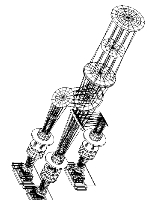
Figure 1: The optical trains of the 2MASS cameras. After the two reflections in the telescope, the first camera element, proceeding from right to left, is the dewar window, followed by a field stop and the first of the seven lenses. Corresponding lenses are identical among the three cameras. Following the first lens (the only one common to all cameras) are the two dichroic mirrors, first $J$ and then $H$. The straight-through light path leads to the $K_{s}$ camera, the upper path to the $J$ camera, and the lower one to $H$.

Our effort to characterize the end-to-end RSRs of 2MASS is based on the transmission data for the various components of the cameras , which appears as part of the Explanatory Supplement for 2MASS. Figure 1 illustrates light paths through the overall instrument, while Table 1 arranges these components from star to detector for each 2MASS band. No end-to-end wavelength-dependent RSRs were measured for the 2MASS system. Therefore, we have constructed these, from the products of the reflection and transmission characteristics of the relevant elements in the optical trains, to yield single files that can be used for synthetic photometry.

The primary and secondary mirrors of the pair of 2MASS telescopes have identical coatings. The plotted curve at the explanatory supplement’s URL is for a single reflection and, therefore, appears squared when one accounts for total system transmission. The transmission of the external dewar window applies identically to the $JHK_{s}$ paths. All three optical paths through the cameras contain seven coated lenses: one common lens ahead of the dichroics and six lenses per channel behind the dichroics. The “Camera Lens Coatings” curve on the Web is for transmission through a single lens element with its coatings. Thus, it is raised to the 7th power to assess the total spectral transmission through each lens assembly. The three dichroic mirrors occur in different combinations of reflection and transmission to provide the distinct light paths for the cameras (Table 1). The $J$, $H$, and $K_{s}$ filter profiles quoted were tested at 77 K. The optical coatings were almost certainly tested at room temperature but the vendor provides no specifications or comparisons to document their behavior at the actual operating temperatures in the 2MASS cameras. The appropriate curves are already flat so that the expected wavelength shifts and shape changes are probably insignificant. The same consideration applies to the dichroic profiles: steep gradients in transmission and/or reflection occur in regions already blocked by the filters.

2.2 The NICMOS3 arrays

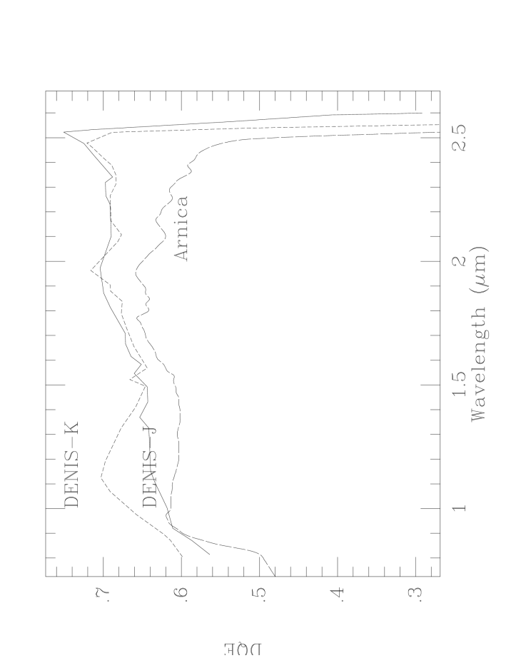
Figure 2: The DQE curves for the actual DENIS $J$ and $K_{s}$ NICMOS3 arrays, and the generic curve supplied with ARNICA.

Adequate data exist within the 2MASS project for all components except for the detector quantum efficiency (hereafter DQE) curves that pertain to the actual 2MASS detector arrays. Only limited work was performed by Rockwell, in general, to characterize DQE as a function of wavelength. No specific characterization was provided for the 2MASS arrays. However, real curves were measured and supplied by Rockwell as part of the characterization and calibration of DENIS (Fouqué  et al. 2000) for 12 regions surrounding the DENIS detectors, in each of the boules that provided the material from which the DENIS $JK_{s}$ detectors were cut. The Arcetri Near-Infrared Camera (ARNICA) also contains a 256$\times$256 NICMOS3 array and was tested in Tucson at the same time as the 2MASS arrays were tested. Dr. L. K. Hunt has kindly provided us with the generic DQE information that she was offered by Rockwell when ARNICA’s array was delivered, and she reports that ARNICA has lower quantum efficiency than the 2MASS devices. Figure 2 compares the actual DQE curves for the DENIS $J$ and $K_{s}$ arrays with the generic information accompanying ARNICA. There are broad similarities between the structure displayed in the curves for all three devices, particularly within the range from 1–2.2 $\mu$m. We have, therefore, chosen to represent the 2MASS DQE curves by the “generic” curve accompanying ARNICA, which was intended as an exemplar of the material used in the 256$\times$256 format. The generic curve clearly satisfies the characteristics of NICMOS3 HgCdTe, as suggested by the DENIS curves. Given our ignorance of the actual 2MASS devices’ performance with wavelength, the qualitative statement that the overall value of the DQE for 2MASS’s arrays exceeds that for ARNICA is not an issue because we will renormalize all derived RSRs so their peaks are unity. We are grateful to Dr. M. F. Skrutskie for locating a set of plots from Rockwell characterizing the HgCdTe material produced at about the same time that the 2MASS NICMOS3 arrays were in production (1996). This documents DQE at 8 locations, albeit for a 1024$\times$1024 array. The curves are in broad agreement with those we offer in Figure 2, and combine the broad plateau seen in ARNICA around 1.3 $\mu$m with the elevated levels of the DENIS arrays beyond 2.0 $\mu$m.

2.3 The contribution of the atmosphere

To represent the intervening telluric transmissions above Mt Hopkins, AZ (MHO) and Cerro Tololo Inter-American Observatory (CTIO) in Chile, we represented the atmospheric transmissions using PLEXUS, an AFRL validated “expert system” that incorporates atmospheric code, specifically MODTRAN 3.7, SAMM, and FASCODE3P with the HITRAN98 archives. PLEXUS contains an extensive database to support its expert aspect, so that the effects of aerosols and particulates appropriate to the desert conditions of the 2MASS sites were included. Paper X also used PLEXUS calculations to represent the site-specific atmospheric transmissions necessary to represent the more than one hundred ground-based filters characterized in that work.

We first verified that the ratio of PLEXUS-computed transmissions at MHO and CTIO was flat over the entire passbands of the $H$ and $K_{s}$ filters, and almost all the $J$ band, and very similar. Therefore, the use of a single calculation to incorporate the atmosphere for both 2MASS telescopes is justified.

2.4 Assembling the RSRs

With the sole exception of the DQE curves, every element in the 2MASS instrument is represented by data germane to the final survey cameras. Strictly, the direct products of all these component curves are valid only if we can ignore the “Stierwalt Effect”. If an interference filter is placed in close proximity to a detector array, the out-of-band-rejection may be greatly changed due to the increased solid angle seen by the detector. Filters are usually measured in a “collimated” beam, the rejected flux being scattered into a larger solid angle. We have explicitly assumed that this effect is not an issue within the 2MASS cameras. Lacking quantitative uncertainties for the characteristics of all these components, we have assigned an overall wavelength-independent error of 5% to the resulting RSRs.

3 2MASS RSRs

Figure 3 presents the three RSRs for 2MASS, including all the optics described above, the (ARNICA) generic DQE curve, and a single PLEXUS atmosphere representative of typical survey conditions. We have followed standard practice by normalizing each RSR to unity at its peak. Note that these RSRs are designed to be integrated directly over stellar spectra in F_λ form, in order to calculate synthetic photometric magnitudes. The quantum efficiency based component was converted to yield photon-counting RSRs by multiplying by $\lambda$ and renormalizing, exactly as described by Bessell (2000). These three RSRs can be found on the Web at: http://www.ipac.caltech.edu/2mass/releases/second/doc/sec3_1b1.tbl12.html ($J$);
http://www.ipac.caltech.edu/2mass/releases/second/doc/sec3_1b1.tbl13.html ($H$);
http://www.ipac.caltech.edu/2mass/releases/second/doc/sec3_1b1.tbl14.html ($K_{s}$), but will soon be moved to analogous URLs on the “allsky” site.

3.1 The influence of water vapor variations

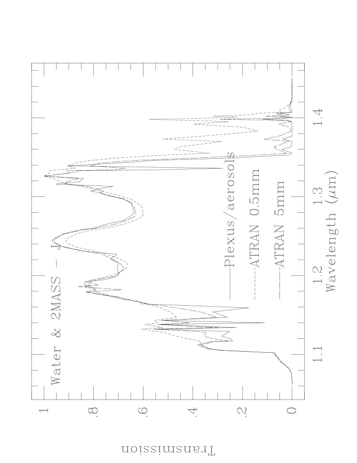
Figure 4: Changes in the 2MASS $J$ RSR due to variations in water vapor.

On some 2MASS survey nights, as much as a 20% variation in response in the $J$-band channel has been seen, presumably due to changes in telluric transmission. Figure 3 indicates that the $J$-band RSR is significantly influenced by water vapor near 1.35 $\mu$m. It is particularly susceptible to intra-night, as well as night-to-night, variations. If all else were unchanged, it is of interest to find out how variable the response might be if it depended solely on the water vapor content of the atmosphere, especially in the $J$-band. Therefore, we investigated the RSRs that would arise as a result of an order of magnitude variation in precipitable water, specifically for amounts of 0.5 and 5 mm. The former would have been a rather rare occurrence during 2MASS operations, while somewhat more than 5 mm would represent the worst conditions under which survey data were collected. These calculations were performed with the ATRAN code (Lord 1992). Calculating for the altitude of MHO, ATRAN predicts about 6.5 mm of precipitable water, but ATRAN enables arbitrary changes, to our selected values of 0.5 and subsequently to 5 mm, without altering any other aspect of the atmosphere (note that, although ATRAN lacks aerosols, particulates, and an expert database, it is a highly flexible code for the study of water vapor variations). Figure 4 illustrates the pair of resulting RSRs. The final adopted $J$ RSR also appears in Figure 4 where it is seen to compare very favorably with the ATRAN transmission curve for 5 mm of water. We still prefer the PLEXUS products because they have been used throughout Paper X, and for DENIS (Fouqué et al. 2000), and because the “expert” mode offers additional realism to our characterization of the atmosphere. The amount of precipitable water vapor in an ATRAN model is not directly comparable to that implied by a PLEXUS model for the same site because of the dependence on the database of actual measurements in PLEXUS, and the inclusion of other phenomena.

No effects were found on the 2MASS $H$ or $K_{s}$ bands due to these gross variations in water vapor.

4 The absolute calibration of 2MASS

To intermingle optical and IR photometry in the normalization of calibrated supertemplates (Paper XIII) requires that every band be well-characterized and that all are integrated over the identical, absolutely calibrated, Kurucz spectrum of Vega published by Cohen et al. (1992), which underpins the entire context of Paper X and, consequently, that of 2MASS and SIRTF too. In the IR we adopt the synthetic Vega spectrum as the definition of zero magnitude, whereas small but nonzero magnitudes apply in the optical (e.g. Bessell et al. 1998; Paper XIII).

Table 2 details the attributes for zero magnitude for 2MASS, giving in-band fluxes, isophotal wavelengths and frequencies, and the corresponding isophotal monochromatic intensities in F_λ and F_ν units, all calculated using the RSRs in this paper. 2MASS $JHK_{s}$ can thereby be transparently compared with photometry in any of the bands in Paper X, and with spectra from all instruments using this common calibration scheme that unifies ground-based, airborne, and spaceborne calibrators. Table 3 offers an estimate of the differences in the absolute calibration of the 2MASS $J$-band for both 0.5 and 5 mm of water, based on the results of constructing RSRs using ATRAN, not PLEXUS. Although the resulting in-band fluxes vary by almost 11%, the isophotal quantities are quite robust in showing only a 2% variation.

Our recommended calibration of 2MASS at $J$ appears in Table 2, based on PLEXUS. Table 3 is shown purely to quantify the impact of isolated water variations on the $J$-band absolute calibration.

5 Zero point offsets

2MASS represents an extremely large body of system magnitudes, defined with respect to an internally homogeneous set of reference stars. Because these stars are not already members of the all-sky network of relatively bright calibrators of Paper X, we require one final step before we can convert 2MASS magnitudes into physical units that are self-consistent with those used by the Diffuse InfraRed Background Explorer, InfraRed Telescope in Space, Kuiper Airborne Observatory, Midcourse Space eXperiment, Infrared Space Observatory, and SIRTF. This step is the definition of the 2MASS ZPOs. The ZPOs are necessary in order to compute absolute quantities using 2MASS magnitudes and Table 2, in the form $10^{-0.4({\it m}+{\it z})}\times~{}F_{\lambda}$(0^m), where m is the observed 2MASS magnitude and z is the algebraic ZPO for that band. Ideally, any photometric system calibrated in the common context of Paper X would be based on the use of any of the more than 600 stars now represented by complete, absolute, 1.2–35 $\mu$m spectra (e.g., those of Paper X). However, the extension of this network to a set of calibrators of intermediate brightness (i.e. $K$=4–10), suitable for use by 2MASS, has occurred only very recently, in readiness for SIRTF. Therefore, we will compute the ZPOs post facto, as the ensemble-averaged algebraic differences between observed and predicted 2MASS $JHK_{s}$ for a set of stars previously absolutely calibrated using other well-characterized NIR data not based on 2MASS.

Paper XIII sets out the procedures by which the suite of IRAC absolute calibrators has been defined, and then applies them to the creation of a set of thirty three 1.2–35 $\mu$m fiducial K0-M0IIIs and A0-A5V stars, drawn from two sets of precision standards: Landolt’s (1992) optical standards, and the Carter & Meadows (1995) optical-NIR photometric stars. These stars now extend the all-sky network described in Paper X downward by factors of 100-1000 in IR brightness. At these levels, they are suitable for cross-ties to 2MASS. The twenty four cool giants are based on $BVRI$ data (supplemented when available by Hipparcos and Tycho data, also calibrated in the common context: see Table 12 in Paper XIII) and on well-characterized $JHK$ measurements either from Tenerife (“TCS”) or South Africa (“SAAO”: see Paper X, Tables 2 and 3). The nine A-dwarfs are based entirely on $BVRIJHK$ data from Carter & Meadows (1995).

By integrating these absolute spectra through the newly-defined 2MASS RSRs and converting the resulting in-band fluxes into magnitudes using Table 2, we have derived the predicted set of 2MASS magnitudes. Direct comparison of these with the final version of observed 2MASS magnitudes enables us to define the “mean algebraic deviation” (hereafter MAD) of a star, by averaging the $JHK_{s}$ differences for that star. Table 4 presents the data for all thirty three stars, giving, for every star: name; spectral type; predicted and observed 2MASS $JHK_{s}$ magnitudes and uncertainties; the differences between these, with their associated errors; and the MAD. The ensemble average MAD results from combining all the (observed-minus-predicted) differences among the thirty three stars, either without weighting (-0.001$\pm$0.005 mag) or using inverse-variance weighting (+0.002$\pm$0.003 mag). We conclude that this set of stars has no significant bias, rendering it ideal to define the 2MASS ZPOs.

The uncertainty used for each observed 2MASS magnitude is the associated $j$, $h$, or “$k\_msigcom$”, i.e. the “complete” error which incorporates the results of processing the photometry, internal errors (from $\surd$N photon statistics and sky background), and calibration errors (nightly zero point, flat fielding, and normalization uncertainties for each band). We were able to use differences for 33 $J$, 30 $H$, and 32 $K_{s}$ magnitudes. $H$-band data for three stars (HD172651 = SA110-471; SA107-35; SA108-827) were rejected because of saturation and/or the concomitant reduced “N out of M” (where only N measurements with aperture photometry above 3$\sigma$ were obtained out of a possible M, a common occurrence for objects on the R1 saturation threshold), or the intrusion of an artifact on one star’s $H$-band image. One $K_{s}$ magnitude (for SA110-471) was rejected from consideration because fewer than 3 non-saturated frames were obtained (“ph_qual”=“E”). All rejected magnitudes and the associated MADs are identified by an asterisk in Table 4.

We have plotted the resulting MADs for the individual stars of the ensemble against spectral type (Figure 5), 2MASS $J-K$ color (Figure 6), and 2MASS $K$ magnitude (Figure 7) and found no perceptible biases with respect to these quantities. The resulting ensemble-averaged ZPOs required to align 2MASS with our common context by algebraically adding them to the final 2MASS magnitudes are: +0.001$\pm$0.005 ($J$); –0.019$\pm$0.007 ($H$); +0.017$\pm$0.005 ($K_{s}$).

6 Conclusions

We have defined element-by-element, photon-counting RSRs for all three 2MASS filter bands, incorporating the properties of detectors, filters, dichroics, lenses, coatings, dewar window, telescopes, and the earth’s atmosphere. The RSRs are absolutely calibrated in the common context of Cohen et al. (1999,2003), and zero point offsets have been developed for 2MASS using thirty three new absolute calibrators of intermediate brightness. 2MASS data are now directly supporting the development of faint calibrators for IRAC and cross-calibrators between pairs of SIRTF instruments using these RSRs to compute synthetic photometry.

Figure 3: The calculated relative spectral response curves for 2MASS bands, renormalized to peak values of unity.

Figure 5: MADs for the ensemble of 33 stars as a function of spectral type.

Figure 6: As Figure 5 but plotted against 2MASS $J-K$ color.

Figure 7: As Figure 5 but plotted against 2MASS $K_{s}$ magnitude.

Table 1: Components of the 2MASS system that have been characterized.

Band	Telescope mirrors	Window	Camera lenses	$J$-dichroic	$H$-dichroic	Filter	DQE	Atmosphere
$J$	primary/secondary	entrance	7 with coatings	reflection	$\cdots$	$J$	generic	PLEXUS
$H$	primary/secondary	entrance	7 with coatings	transmission	reflection	$H$	generic	PLEXUS
$K_{s}$	primary/secondary	entrance	7 with coatings	transmission	transmission	$K_{s}$	generic	PLEXUS

Table 2: Zero magnitude attributes of 2MASS bands.

Filter	Bandwidth	In-Band	Fλ(iso)	$\lambda$(iso)	Bandwidth	Fν(iso)	$\nu$(iso)
	$\mu$m	W cm-2	W cm-2 $\mu$m-1	$\mu$m	Hz	Jy	Hz
	Uncertainty	Uncertainty	Uncertainty	Uncertainty	Uncertainty	Uncertainty	Uncertainty
	$\mu$m	%	W cm-2 $\mu$m-1	$\mu$m	Hz	Jy	Hz
$J$	0.162	5.082E-14	3.129E-13	1.235	3.189E+13	1594	2.428E+14
	0.001	1.608	5.464E-15	0.006	2.155E+11	27.80	2.746E+12
$H$	0.251	2.843E-14	1.133E-13	1.662	2.778E+13	1024	1.783E+14
	0.002	1.721	2.212E-15	0.009	2.540E+11	19.95	2.139E+12
$K_{s}$	0.262	1.122E-14	4.283E-14	2.159	1.682E+13	666.7	1.390E+14
	0.002	1.685	8.053E-16	0.011	1.409E+11	12.55	1.496E+12

Table 3: Zero magnitude attributes of 2MASS $J$-band under different water vapor conditions.

Water	Bandwidth	In-Band	Fλ(iso)	$\lambda$(iso)
mm	$\mu$m	W cm-2	W cm-2 $\mu$m-1	$\mu$m
	Uncertainty	Uncertainty	Uncertainty	Uncertainty
	$\mu$m	W cm-2	W cm-2 $\mu$m-1	$\mu$m
5	0.170	5.319E-14	3.127E-13	1.235
	0.001	8.507E-16	2.901E-15	0.003
0.5	0.192	5.888E-14	3.060E-13	1.243
	0.001	9.321E-16	2.638E-15	0.003

Table 4: Predicted and observed 2MASS $JHK_{s}$ for Landolt and Carter-Meadows stars. Magnitudes and differences marked by asterisks were rejected as discussed in the text.

HD	SA/SAO	Type	Predicted $J$	Observed $J$	Difference	Predicted $H$	Observed $H$	Difference	Predicted $K_{s}$	Observed $K_{s}$	Difference	MAD
HD5319	SA92-336	K0III	6.323$\pm$0.011	6.348$\pm$0.027	+0.025$\pm$0.029	5.838$\pm$0.009	5.864$\pm$0.044	+0.026$\pm$0.045	5.735$\pm$0.008	5.699$\pm$0.020	–0.036$\pm$0.022	+0.005
$\cdots$	SA94-251	K1III	9.063$\pm$0.020	9.003$\pm$0.027	–0.060$\pm$0.034	8.459$\pm$0.018	8.425$\pm$0.051	–0.034$\pm$0.054	8.311$\pm$0.016	8.284$\pm$0.033	–0.027$\pm$0.037	–0.040
$\cdots$	SA103-526	K0III	9.016$\pm$0.016	9.020$\pm$0.019	+0.004$\pm$0.025	8.506$\pm$0.013	8.475$\pm$0.053	–0.031$\pm$0.055	8.386$\pm$0.013	8.362$\pm$0.031	–0.024$\pm$0.033	–0.017
HD118280	SA105-205	K3III	6.366$\pm$0.010	6.343$\pm$0.020	–0.023$\pm$0.023	5.703$\pm$0.008	5.726$\pm$0.034	+0.023$\pm$0.035	5.466$\pm$0.007	5.445$\pm$0.017	–0.021$\pm$0.018	–0.007
HD118290	SA105-405	K5III	5.615$\pm$0.009	5.597$\pm$0.024	–0.018$\pm$0.026	4.851$\pm$0.007	4.879$\pm$0.059	+0.028$\pm$0.059	4.619$\pm$0.006	4.638$\pm$0.016	+0.019$\pm$0.017	+0.010
HD139308	SA107-35	K2III	5.607$\pm$0.011	5.609$\pm$0.034	+0.002$\pm$0.036	4.935$\pm$0.009	∗5.058$\pm$0.040	∗0.123$\pm$0.041	4.821$\pm$0.009	4.809$\pm$0.024	–0.012$\pm$0.026	–0.005
HD139513	SA107-347	K1.5III	7.058$\pm$0.017	7.045$\pm$0.021	–0.013$\pm$0.027	6.414$\pm$0.010	6.328$\pm$0.034	–0.086$\pm$0.035	6.270$\pm$0.009	6.182$\pm$0.022	–0.088$\pm$0.024	–0.062
$\cdots$	SA107-484	K3III	9.151$\pm$0.014	9.170$\pm$0.021	+0.019$\pm$0.025	8.525$\pm$0.012	8.512$\pm$0.042	–0.013$\pm$0.044	8.311$\pm$0.010	8.431$\pm$0.044	+0.120$\pm$0.045	+0.042
$\cdots$	SA108-475	K3III	8.845$\pm$0.015	8.828$\pm$0.019	–0.017$\pm$0.024	8.174$\pm$0.012	8.148$\pm$0.036	–0.026$\pm$0.038	7.933$\pm$0.010	7.990$\pm$0.024	+0.057$\pm$0.026	+0.005
HD149845	SA108-827	K2III	5.744$\pm$0.012	5.738$\pm$0.032	–0.006$\pm$0.034	5.062$\pm$0.010	∗5.187$\pm$0.017	∗0.125$\pm$0.020	4.943$\pm$0.009	4.935$\pm$0.018	–0.008$\pm$0.020	–0.007
$\cdots$	SA108-1918	K3III	8.840$\pm$0.015	8.868$\pm$0.025	+0.028$\pm$0.029	8.154$\pm$0.012	8.128$\pm$0.038	–0.026$\pm$0.040	7.903$\pm$0.011	7.959$\pm$0.036	+0.056$\pm$0.038	+0.019
$\cdots$	SA109-231	K2III	6.746$\pm$0.015	6.700$\pm$0.021	–0.046$\pm$0.026	6.012$\pm$0.012	6.050$\pm$0.033	+0.038$\pm$0.035	5.862$\pm$0.011	5.862$\pm$0.022	+0.000$\pm$0.025	–0.003
HD172651	SA110-471	K2III	4.933$\pm$0.011	4.930$\pm$0.019	–0.003$\pm$0.022	4.204$\pm$0.009	∗3.876$\pm$0.220	∗-0.328$\pm$0.220	4.055$\pm$0.008	∗4.079$\pm$0.036	∗0.024$\pm$0.037	–0.003
$\cdots$	SA112-275	K0III	7.749$\pm$0.015	7.791$\pm$0.029	+0.042$\pm$0.033	7.199$\pm$0.012	7.197$\pm$0.036	–0.002$\pm$0.038	7.055$\pm$0.011	7.058$\pm$0.024	+0.003$\pm$0.026	+0.014
$\cdots$	SA112-595	M0III	8.361$\pm$0.014	8.341$\pm$0.021	–0.020$\pm$0.025	7.486$\pm$0.011	7.502$\pm$0.042	+0.016$\pm$0.043	7.289$\pm$0.010	7.296$\pm$0.026	+0.007$\pm$0.028	+0.001
$\cdots$	SA113-259	K2III	9.745$\pm$0.018	9.725$\pm$0.023	–0.020$\pm$0.029	9.099$\pm$0.016	9.132$\pm$0.021	+0.033$\pm$0.027	9.002$\pm$0.016	8.994$\pm$0.026	–0.008$\pm$0.030	+0.001
$\cdots$	SA113-269	K0III	7.548$\pm$0.014	7.589$\pm$0.021	+0.041$\pm$0.025	7.030$\pm$0.011	7.010$\pm$0.042	–0.020$\pm$0.043	6.906$\pm$0.010	6.879$\pm$0.017	–0.027$\pm$0.020	–0.002
HD215141	SA114-176	K4III	6.673$\pm$0.014	6.618$\pm$0.021	–0.055$\pm$0.025	5.942$\pm$0.012	5.946$\pm$0.029	+0.004$\pm$0.031	5.729$\pm$0.010	5.734$\pm$0.018	+0.005$\pm$0.021	–0.015
$\cdots$	SA114-548	K3III	9.187$\pm$0.015	9.300$\pm$0.026	+0.113$\pm$0.030	8.524$\pm$0.012	8.528$\pm$0.040	+0.004$\pm$0.042	8.287$\pm$0.011	8.378$\pm$0.026	+0.091$\pm$0.028	+0.069
$\cdots$	SA114-656	K1III	10.841$\pm$0.022	10.815$\pm$0.026	–0.026$\pm$0.034	10.290$\pm$0.020	10.301$\pm$0.021	+0.011$\pm$0.029	10.174$\pm$0.019	10.197$\pm$0.021	+0.023$\pm$0.028	+0.003
$\cdots$	SA114-670	K1.5III	8.950$\pm$0.020	9.016$\pm$0.024	+0.066$\pm$0.029	8.336$\pm$0.013	8.390$\pm$0.027	+0.054$\pm$0.031	8.210$\pm$0.012	8.279$\pm$0.026	+0.069$\pm$0.028	+0.063
HD222732	SA115-427	K2III	6.860$\pm$0.013	6.857$\pm$0.021	–0.003$\pm$0.025	6.216$\pm$0.011	6.214$\pm$0.026	–0.002$\pm$0.028	6.119$\pm$0.011	6.104$\pm$0.022	–0.015$\pm$0.025	–0.007
$\cdots$	SA115-516	K1.5III	8.506$\pm$0.018	8.522$\pm$0.021	+0.016$\pm$0.027	7.927$\pm$0.011	7.948$\pm$0.024	+0.021$\pm$0.027	7.822$\pm$0.011	7.851$\pm$0.021	+0.029$\pm$0.024	+0.022
HD197806	$\cdots$	K0III	7.563$\pm$0.014	7.585$\pm$0.024	+0.022$\pm$0.028	7.022$\pm$0.012	7.027$\pm$0.044	+0.005$\pm$0.046	6.884$\pm$0.011	6.849$\pm$0.031	–0.035$\pm$0.033	–0.002
HD15911	SAO232803	A0V	9.439$\pm$0.035	9.430$\pm$0.023	–0.009$\pm$0.042	9.483$\pm$0.041	9.497$\pm$0.023	+0.014$\pm$0.047	9.450$\pm$0.043	9.421$\pm$0.019	–0.029$\pm$0.047	–0.008
HD29250	SAO169590	A4V	9.419$\pm$0.036	9.425$\pm$0.026	+0.006$\pm$0.045	9.386$\pm$0.041	9.383$\pm$0.027	–0.003$\pm$0.049	9.322$\pm$0.042	9.308$\pm$0.026	–0.014$\pm$0.050	–0.003
HD62388	SAO153304	A0V	8.715$\pm$0.033	8.702$\pm$0.025	–0.013$\pm$0.042	8.734$\pm$0.038	8.684$\pm$0.040	–0.050$\pm$0.055	8.686$\pm$0.040	8.657$\pm$0.019	–0.029$\pm$0.044	–0.030
HD71264	SAO135911	A0V	8.572$\pm$0.034	8.603$\pm$0.030	+0.031$\pm$0.045	8.572$\pm$0.038	8.571$\pm$0.024	–0.001$\pm$0.045	8.512$\pm$0.040	8.577$\pm$0.023	+0.065$\pm$0.046	+0.032
HD84090	SAO221405	A3V	8.534$\pm$0.032	8.546$\pm$0.027	+0.012$\pm$0.042	8.531$\pm$0.037	8.500$\pm$0.047	–0.031$\pm$0.060	8.477$\pm$0.038	8.482$\pm$0.023	+0.005$\pm$0.045	–0.004
HD105116	SAO223215	A2V	8.143$\pm$0.032	8.117$\pm$0.024	–0.026$\pm$0.040	8.126$\pm$0.036	8.033$\pm$0.027	–0.093$\pm$0.045	8.060$\pm$0.037	7.999$\pm$0.020	–0.061$\pm$0.042	–0.060
HD106807	SAO223331	A1V	8.698$\pm$0.033	8.667$\pm$0.021	–0.031$\pm$0.040	8.704$\pm$0.038	8.693$\pm$0.026	–0.011$\pm$0.046	8.648$\pm$0.039	8.652$\pm$0.025	+0.004$\pm$0.047	–0.013
HD136879	SAO253162	A0V	8.615$\pm$0.035	8.613$\pm$0.029	–0.002$\pm$0.045	8.620$\pm$0.039	8.556$\pm$0.045	–0.046$\pm$0.060	8.535$\pm$0.040	8.541$\pm$0.021	+0.006$\pm$0.045	–0.014
HD216009	SAO231319	A0V	7.961$\pm$0.030	7.957$\pm$0.024	–0.004$\pm$0.038	7.988$\pm$0.034	7.966$\pm$0.042	–0.022$\pm$0.054	7.945$\pm$0.036	7.913$\pm$0.027	–0.032$\pm$0.045	–0.020

References

- (1) Bessell, M.S. 2000, PASP, 112, 961
- (2) Bessell, M.S., Castelli, F., & Plez, B. 1998, A&A, 333, 231
- (3) Carter, B.S. & Meadows, V.S. 1995, MNRAS, 276, 734
- (4) Cohen, M., Megeath, S. T., Hammersley, P. L., Martin-Luis, F., & Stauffer, J. 2003, AJ, in press (May 2003) (Paper XIII)
- (5) Cohen, M., Walker, R. G., Barlow, M. J. & Deacon, J. R. 1992, AJ, 104, 1650
- (6) Cohen, M., Walker, R. G., Carter, B., Hammersley, P. L., Kidger, M. R., & Noguchi, K. 1999, AJ, 117, 1864 (Paper X)
- (7) Fouqué , P. et al. 2000, A&AS, 141, 313
- (8) Kurucz, R.L. 1993, CDROMs, ATLAS9 Stellar Atmospheres’ Programs and 2 km s-1 Grid (Cambridge: Smithsonian Astrophysical Observatory)
- (9) Landolt, A.U. 1992, AJ,104, 340
- (10) Lord, S. D. 1992, A New Software Tool for Computing the Earth’s Atmospheric Transmission of Near-Infrared and Far-Infrared Radiation, NASA TM-103957
- (11) Walker, R.G. & Cohen, M. 2002, “Walker-Cohen Atlas of Calibrated Spectra, Explanatory Supplement to Release 4.0”, Contractor’s Report to USAF Phillips Laboratory, Contract F19628-98-C-0047