Local Radiative Hydrodynamic and Magnetohydrodynamic Instabilities in Optically Thick Media

Abstract

We examine the local conditions for radiative damping and driving of short wavelength, propagating hydrodynamic and magnetohydrodynamic (MHD) waves in static, optically thick, stratified equilibria. We show that so-called strange modes in stellar oscillation theory and magnetic photon bubbles are intimately related and are both fundamentally driven by the background radiation flux acting on compressible waves. We identify the necessary criteria for unstable driving of these waves, and show that this driving can exist in both gas and radiation pressure dominated media, as well as pure Thomson scattering media in the MHD case. The equilibrium flux acting on opacity fluctuations can drive both hydrodynamic acoustic waves and magnetosonic waves unstable. In addition, magnetosonic waves can be driven unstable by a combination of the equilibrium flux acting on density fluctuations and changes in the background radiation pressure along fluid displacements. We briefly describe the conditions under which these instabilities might be manifested in both main sequence stellar envelopes and accretion disks.

1 Introduction

It is well known that the presence of a substantial equilibrium radiation pressure gradient can destabilize optically thick astrophysical media. Prendergast & Spiegel (1973) first speculated that compressible fluid flow subject to a large radiative flux would be unstable to the formation of buoyant rarefied regions of enhanced radiation pressure, better known as “photon bubbles.” The existence of these instabilities has never been fully demonstrated in hydrodynamic systems, but radiation pressure acting in stellar envelopes with opacity peaks can drive certain oscillation modes (now known as “strange modes”) unstable (e.g. Wood 1976; Saio, Wheeler, & Cox 1984; Gautschy 1993; Kiriakidis, Fricke, & Glatzel 1993). Strange modes have also been found to exist in hydrodynamic models of accretion disks (Glatzel & Mehren 1996, Mehren-Baehr & Glatzel 1999).

Gautschy & Glatzel (1990) showed that strange mode instabilities satisfy a “non-adiabatic reversible” (NAR) approximation, in which the modes occur in a medium with effectively zero specific heat capacity, resulting in a vanishing luminosity perturbation. A physical model for strange mode instabilities within the NAR approximation was established by Glatzel (1994). He noted that opacity peaks act as a reflection barrier for high overtone acoustic modes, sonically decoupling different radial regions in the star. The basic mechanism for the instability was the relative phase shift between the pressure and density perturbations, resulting from the constraint of having zero luminosity perturbation. Further aspects of the physics of strange modes have been elucidated by Papaloizou et al. (1997) and Saio, Baker, & Gautschy (1998). In numerical studies, Shaviv (2001) has found that both standing and propagating acoustic waves are unstable in atmospheres with sufficient radiation pressure support, even when the opacity is pure Thomson scattering.

Radiation pressure driven instabilities occur in magnetized systems as well. Arons (1992) identified and investigated photon bubble instabilities in strongly magnetized atmospheres of accreting X-ray pulsars. He showed that such instabilities are caused by the enhanced buoyancy that occurs when radiation diffuses into relatively rarefied regions in compressible perturbations. With accretion disk applications in mind, Gammie (1998) performed a linear, local stability analysis of a static, magnetized, stratified medium and found an instability over a finite range of wavenumbers that he identified as being similar in nature to photon bubbles. Using the simplifying assumption that gas and radiation were coupled together just by Thomson scattering, Blaes & Socrates (2001, hereafter BS01) found that Gammie’s (1998) instability could be extended to arbitrarily short wavelengths where it manifested itself as an overstable slow mode. In addition, the fast magnetosonic mode could also be unstable for sufficiently strong radiation fluxes, albeit with smaller growth rate. Begelman (2001) has constructed a periodic shock train solution that may represent one possible nonlinear outcome of the slow mode instability.

The purpose of this paper is to investigate the local, WKB version of these compressive instabilities in a unified manner. We focus on the local driving of propagating waves, and do not address here the issue of whether and how this local driving can manifest itself as a global instability of a standing, normal mode of the object in question. We treat the thermodynamics of the medium quite generally, making no restrictive assumptions on the equality of the gas and radiation temperature in the perturbed state or using the NAR approximation. We find that hydrodynamic instabilities driven by radiative diffusion exist under a wide range of conditions, for both gas and radiation pressure dominated media. However, a medium supported purely by Thomson scattering opacity exhibits no local driving of acoustic wave instabilities, in contrast to the conclusions of Shaviv (2001). On the other hand, the anisotropic stress produced by magnetic tension widens the applicability of these instabilities to even broader classes of equilibria, even those which have opacities given by Thomson scattering only. The MHD instabilities can exist even when the equilibrium magnetic pressure is less than either the gas or radiation pressure.

All these instabilities may grow on the dynamical time scale or even faster. The instability mechanism originates from the interaction of the equilibrium radiative flux with density and opacity fluctuations in the perturbed flow, as well as changes in radiation pressure along fluid displacements. The ultimate source of free energy is provided by the stratified radiation field.

This paper is organized as follows. In section 2, we describe our basic equations and assumptions, concentrating in particular on the thermodynamics of the coupled gas and radiation fluids, and also derive the general dispersion relation for waves in a stratified, magnetized medium within the local (WKB) limit. In section 3 we discuss the solutions of this dispersion relation in the hydrodynamic limit where there is no magnetic field, generalizing and extending the work of previous authors. We discuss in some detail the physics underlying these instabilities in section 4. We then incorporate the effects of magnetic fields in section 5, and in section 6 discuss how the physics of magnetoacoustic wave instabilities is related to the hydrodynamic instabilities of the previous sections. In section 7 we briefly discuss astrophysical applications of these instabilities to accretion disks and stars, deferring more detailed applications to observed phenomena for future work. Section 8 summarizes our main conclusions. Our WKB analysis in the main body of the paper is not completely rigorous, and we provide more solid mathematical justification for our conclusions for two particular cases in an appendix. We also include an additional appendix where we examine the effects of radiative diffusion on the magnetorotational (MRI) instability in differentially rotating flows, generalizing our previous work (BS01) to include the more generic thermodynamics we use here. Readers not interested in the details of the linear perturbation theory may wish to skip ahead to sections 7 and 8 directly. Readers interested in obtaining a basic physical understanding of the causes of these instabilities may wish to focus on sections 4 and 6.

2 Equations and Assumptions

The basic equations of radiation magnetohydrodynamics (RMHD) have been discussed by Stone, Mihalas, & Norman (1992), and we adopt these equations here with slight changes in notation as well as some changes in the physics. The fluid equations we consider are

$${\partial\rho\over\partial t}+{\hbox{{\syvec\char 114\relax}}\cdot}(\rho{\bf v})=0,$$ (1)

$$\rho\left({\partial{\bf v}\over\partial t}+{\bf v\cdot\hbox{{\syvec\char 114\relax}}v}\right)=-{\hbox{{\syvec\char 114\relax}}}p+\rho{\bf g}+{1\over 4\pi}({\bf\hbox{{\syvec\char 114\relax}}\times B}){\bf\times B}+{\kappa_{\rm F}\rho\over c}{\bf F},$$ (2)

$${\partial u\over\partial t}+{\bf v\cdot\hbox{{\syvec\char 114\relax}}}u+\gamma u{\bf\hbox{{\syvec\char 114\relax}}\cdot v}=\kappa_{\rm J}\rho cE-\kappa_{\rm P}\rho caT_{\rm g}^{4}-\kappa_{\rm T}\rho c\left({4k_{\rm B}T_{\rm g}\over m_{\rm e}c^{2}}-{h\bar{\nu}\over m_{\rm e}c^{2}}\right)E,$$ (3)

$${\partial E\over\partial t}+{\bf v\cdot\hbox{{\syvec\char 114\relax}}}E+{4\over 3}E{\bf\hbox{{\syvec\char 114\relax}}\cdot v}=-{\bf\hbox{{\syvec\char 114\relax}}\cdot F}-\kappa_{\rm J}\rho cE+\kappa_{\rm P}\rho caT_{\rm g}^{4}+\kappa_{\rm T}\rho c\left({4k_{\rm B}T_{\rm g}\over m_{\rm e}c^{2}}-{h\bar{\nu}\over m_{\rm e}c^{2}}\right)E,$$ (4)

$$0=-{1\over 3}{\hbox{{\syvec\char 114\relax}}}E-{\kappa_{\rm F}\rho\over c}{\bf F},$$ (5)

and

$${\partial{\bf B}\over\partial t}={\hbox{{\syvec\char 114\relax}}\times}({\bf v\times B}).$$ (6)

Here $\rho$, $p$, $T_{\rm g}$, and $u$ are the density, pressure, temperature, and energy density in the gas, respectively. These quantities are related to each other by

$$u={p\over\gamma-1}$$ (7)

and

$$p={\rho k_{\rm B}T_{\rm g}\over\mu},$$ (8)

where $\gamma$ is the ratio of specific heats in the gas and $\mu$ is the mean molecular mass of the gas. We assume throughout this paper that $\gamma$ and $\mu$ are constant, and thereby neglect the effects of composition gradients, ionization, and recombination.

Other symbols in equations (1)-(8) have their usual meaning: $c$ is the speed of light, $a$ is the radiation density constant, $k_{\rm B}$ is Boltzmann’s constant, and $m_{\rm e}$ is the electron mass. The vector ${\bf v}$ is the fluid velocity, ${\bf B}$ is the magnetic field, and ${\bf g}$ is the gravitational acceleration. We assume that ${\bf g}$ is time-independent throughout this paper, either because the gravitational field is due to some fixed external source (as is the case for a non-self-gravitating accretion disk), or because we choose to consider only short-wavelength perturbations that are well-described by the Cowling approximation.

The radiation energy density $E$ and the radiation flux ${\bf F}$ are defined in terms of frequency integrals over the radiation spectrum as measured in the local fluid rest frame:

$$E\equiv{4\pi\over c}\int_{0}^{\infty}d\nu J_{\nu}\equiv{4\pi\over c}J,$$ (9)

where $J_{\nu}$ is the angle-averaged mean specific intensity in the local fluid rest frame, and

$${\bf F}\equiv\int_{0}^{\infty}d\nu{\bf F}_{\nu}.$$ (10)

We have simplified the RMHD equations by assuming that the radiation stress tensor is isotropic in the local fluid rest frame, i.e. that the tensor variable Eddington factor defined by Stone et al. (1992) is one third times the identity matrix. We have therefore neglected the effects of photon viscosity. We have also neglected terms corresponding to radiation inertia in the radiation momentum equation (5), leaving us with just the radiation diffusion equation. Such terms are generally negligible for the low frequency instabilities we explore in this paper (e.g. BS01).

The two opacities $\kappa_{\rm J}$ and $\kappa_{\rm F}$ are also defined by integrals over the radiation spectrum in the local rest frame:

$$\kappa_{\rm J}\equiv{1\over\rho J}\int_{0}^{\infty}d\nu\chi_{\nu}^{\rm th}(\rho,T_{\rm g})J_{\nu},$$ (11)

and

$$\kappa_{\rm F}{\bf F}\equiv{1\over\rho}\int_{0}^{\infty}d\nu[\chi_{\nu}^{\rm th}(\rho,T_{\rm g})+n_{\rm e}\sigma_{\rm T}]{\bf F}_{\nu}.$$ (12)

Here $\chi_{\nu}^{\rm th}(\rho,T_{\rm g})$ is the thermal absorption coefficient at frequency $\nu$, $n_{\rm e}$ is the electron number density, and $\sigma_{\rm T}$ is the Thomson cross-section. The Planck mean opacity is

$$\kappa_{\rm P}\equiv{4\pi\over\rho acT_{\rm g}^{4}}\int_{0}^{\infty}d\nu\chi_{\nu}^{\rm th}(\rho,T_{\rm g})B_{\nu}(T_{\rm g}),$$ (13)

where $B_{\nu}(T_{\rm g})$ is the Planck function at the gas temperature. The Thomson opacity is

$$\kappa_{\rm T}\equiv{n_{e}\sigma_{\rm T}\over\rho}$$ (14)

and is constant due to our neglect of ionization/recombination processes and composition gradients. Note that we have extended the RMHD equations of Stone et al. (1992) to include electron scattering. Coherent (Thomson) scattering merely allows the gas and radiation to exchange momentum, not energy. However, we have also allowed for incoherent (Compton) scattering in the last terms on the right hand side of the gas and radiation energy equations (3) and (4). We do this by treating Compton scattering in the frequency diffusion (Kompaneets) limit, neglecting anisotropies in the radiation field in the local fluid rest frame. A derivation of the Compton scattering terms can be found, e.g., in section 3.1 of Hubeny et al. (2001). The quantity $\bar{\nu}$ is an average frequency of the radiation field in the local rest frame of the fluid, defined by

$$\bar{\nu}\equiv{1\over J}\int_{0}^{\infty}d\nu\nu J_{\nu}\left(1+{J_{\nu}c^{2}\over 2h\nu^{3}}\right).$$ (15)

The second term in parentheses represents the effects of stimulated scattering, and guarantees that there is no net heat exchange between the gas and the radiation when thermal equilibrium is established with the radiation field being blackbody at the local gas temperature.

In principle, evaluation of the frequency integrals in the opacities and $\bar{\nu}$ requires a full solution of the radiative transfer equation coupled to the fluid flow. Rather than do that here, we adopt some simplified prescriptions that we believe will not alter the essential physics we wish to explore. First, we adopt the Eddington closure relation between the zeroth and second moments of the comoving frame specific intensity, consistent with our earlier assumption that the tensor variable Eddington factor is one third times the identity matrix. Second, because we will only consider perturbations about equilibria that are in local thermodynamic equilibrium (LTE), we assume that non-LTE departures in the perturbed flow can be adequately parameterized by a blackbody radiation spectrum at a temperature $T_{\rm r}$, which may be different from the gas temperature $T_{\rm g}$.

Under these assumptions, equation (15) implies that

$$\bar{\nu}={4k_{\rm B}T_{\rm r}\over h}.$$ (16)

Equation (11) gives an expression for $\kappa_{\rm J}$ which more closely resembles the Planck mean opacity $\kappa_{\rm P}$,

$$\kappa_{\rm J}={4\pi\over\rho acT_{\rm r}^{4}}\int_{0}^{\infty}d\nu\chi_{\nu}^{\rm th}(\rho,T_{\rm g})B_{\nu}(T_{\rm r}).$$ (17)

In addition, equation (12) can be replaced with an expression analogous to the Rosseland mean opacity,

$$\kappa_{\rm F}=\left(\int_{0}^{\infty}d\nu{dB_{\nu}\over dT_{\rm r}}\right)\left\{\int_{0}^{\infty}d\nu\left[{\chi_{\nu}^{\rm th}(\rho,T_{\rm g})\over\rho}+\kappa_{\rm T}\right]^{-1}{dB_{\nu}\over dT_{\rm r}}\right\}^{-1}.$$ (18)

Unlike $\kappa_{\rm P}$, which is a function only of the gas density and temperature, $\kappa_{\rm J}$ and $\kappa_{\rm F}$ are also functions of the radiation temperature. Finally, the blackbody assumption implies that $T_{\rm r}$ can be related to the radiation energy density through the equation of state

$$E=aT_{\rm r}^{4}.$$ (19)

To summarize, equations (1)-(8), (13), and (16)-(19) are the basic dynamical equations we will use throughout the rest of this paper.

2.1 Equilibrium

For the majority of this paper we will consider the dynamical stability of static equilibria in which the equilibrium fluid velocity is zero. As mentioned in the previous section, we also assume that the equilibrium is in LTE, i.e. that the unperturbed gas and radiation temperatures are identical,

$$T_{\rm g}=T_{\rm r}\equiv T.$$ (20)

This can be somewhat problematic for applications to accretion disk models, which in some cases can be effectively thin. However, we do not presume to model the turbulent dissipation that must exist in these flows. In fact, our purpose in that application is to consider equilibria that might be useful starting points for exploring the development of this turbulence by simulation. Lacking an explicit treatment of dissipation, we are forced to consider equilibria that are in LTE and in local radiative equilibrium.

Under these assumptions, the only nontrivial partial differential equations describing our equilibrium are those expressing hydrostatic equilibrium,

$$0=\rho{\bf g}-{\hbox{{\syvec\char 114\relax}}}p+{1\over 4\pi}({\bf\hbox{{\syvec\char 114\relax}}\times B}){\bf\times B}+{\kappa_{\rm F}\rho\over c}{\bf F},$$ (21)

radiative equilibrium,

$$0={\hbox{{\syvec\char 114\relax}}}\cdot{\bf F},$$ (22)

and radiative diffusion,

$$0=-{1\over 3}{\hbox{{\syvec\char 114\relax}}}E-{\kappa_{\rm F}\rho\over c}{\bf F}.$$ (23)

Throughout this paper we will assume that the equilibrium magnetic field is uniform, so that the Lorentz force term in equation (21) vanishes. Equation (21) then has the immediate consequence that all thermodynamic variables are constant on horizontal surfaces, i.e. those surfaces that are perpendicular to the gravitational acceleration ${\bf g}$. We define $z$ to be a vertical coordinate that increases upward, and $\hat{\bf z}$ to be the corresponding upward unit vector. Then ${\bf g}\equiv-g\hat{\bf z}$, with $g>0$.

2.2 The Linear Perturbation in Total Pressure

When we consider the behavior of linear perturbations about the equilibrium just discussed, the problem naturally divides into two parts: the thermodynamics of the perturbed flow, and the coupling of this with the perturbed magnetic and velocity fields. We examine the former problem first by determining the perturbed total (gas plus radiation) pressure.

We begin by considering expressions for the perturbations in $\kappa_{\rm J}$ and $\kappa_{\rm P}$. The functional dependence of these two opacities on $\rho$, $T_{\rm g}$ and $T_{\rm r}$ immediately implies that

$${\delta\kappa_{\rm J}\over\kappa_{\rm J}}={\partial\ln\kappa_{\rm J}\over\partial\ln\rho}{\delta\rho\over\rho}+{\partial\ln\kappa_{\rm J}\over\partial\ln T_{\rm g}}{\delta T_{\rm g}\over T_{\rm g}}+{\partial\ln\kappa_{\rm J}\over\partial\ln T_{\rm r}}{\delta T_{\rm r}\over T_{\rm r}}$$ (24)

and

$${\delta\kappa_{\rm P}\over\kappa_{\rm P}}={\partial\ln\kappa_{\rm P}\over\partial\ln\rho}{\delta\rho\over\rho}+{\partial\ln\kappa_{\rm P}\over\partial\ln T_{\rm g}}{\delta T_{\rm g}\over T_{\rm g}}.$$ (25)

(We use Eulerian perturbations throughout this paper, i.e. $\delta Q$ is the Eulerian perturbation in the quantity $Q$.) Here all opacity derivatives are evaluated in the equilibrium state which is in LTE with $T_{\rm r}=T_{\rm g}$ and $\kappa_{\rm P}=\kappa_{\rm J}$. Because of this, equations (13) and (17) immediately imply

$${\partial\ln\kappa_{\rm P}\over\partial\ln\rho}={\partial\ln\kappa_{\rm J}\over\partial\ln\rho}$$ (26)

and

$${\partial\ln\kappa_{\rm P}\over\partial\ln T_{\rm g}}={\partial\ln\kappa_{\rm J}\over\partial\ln T_{\rm g}}+{\partial\ln\kappa_{\rm J}\over\partial\ln T_{\rm r}}.$$ (27)

These two conditions on the absorption opacity derivatives greatly simplify the mathematical form of the thermal coupling between the gas and radiation in the perturbed flow. Linearizing the gas energy equation (3) and the radiation energy equation (4), and using equations (16), (19), and (26)-(27), we obtain

$${\partial\delta u\over\partial t}+\delta{\bf v}\cdot{\hbox{{\syvec\char 114\relax}}}u+\gamma u{\hbox{{\syvec\char 114\relax}}}\cdot\delta{\bf v}=\omega_{\rm a}E{4(\delta T_{\rm r}-\delta T_{\rm g})\over T}$$ (28)

and

$${\partial\delta E\over\partial t}+\delta{\bf v}\cdot{\hbox{{\syvec\char 114\relax}}}E+{4\over 3}E{\hbox{{\syvec\char 114\relax}}}\cdot\delta{\bf v}=-{\hbox{{\syvec\char 114\relax}}}\cdot\delta{\bf F}-\omega_{\rm a}E{4(\delta T_{\rm r}-\delta T_{\rm g})\over T}.$$ (29)

Here $\omega_{\rm a}$ is an angular frequency describing the rate at which radiation and matter are thermally coupled in the perturbed flow, defined by

$$\omega_{\rm a}\equiv\left[\kappa_{\rm P}\left(1+{1\over 4}{\partial\ln\kappa_{\rm J}\over\partial\ln T_{\rm r}}\right)+\kappa_{\rm T}{k_{\rm B}T\over m_{\rm e}c^{2}}\right]\rho c\equiv\kappa_{\rm a}\rho c.$$ (30)

Equations (28) and (29) can be further manipulated in a physically revealing manner. We eliminate ${\hbox{{\syvec\char 114\relax}}}\cdot\delta{\bf v}$ from them using the perturbed continuity equation (1),

$${\partial\delta\rho\over\partial t}+\rho{\hbox{{\syvec\char 114\relax}}}\cdot\delta{\bf v}+\delta{\bf v}\cdot{\hbox{{\syvec\char 114\relax}}}\rho=0.$$ (31)

In addition, we eliminate $\delta{\bf F}$ using the perturbed radiative diffusion equation (5), which can be written as

$$\delta{\bf F}=-{c\over 3\kappa_{\rm F}\rho}{\hbox{{\syvec\char 114\relax}}}\delta E-{\bf F}\left({\delta\rho\over\rho}+{\delta\kappa_{\rm F}\over\kappa_{\rm F}}\right).$$ (32)

Eliminating $\delta u$ using equation (7), equation (28) becomes

$${\partial\delta p\over\partial t}-c_{\rm g}^{2}{\partial\delta\rho\over\partial t}=4(\gamma-1)\omega_{\rm a}E{(\delta T_{\rm r}-\delta T_{\rm g})\over T}-(\gamma-1)\rho T\delta{\bf v}\cdot{\hbox{{\syvec\char 114\relax}}}S_{\rm g},$$ (33)

where $c_{\rm g}$ is the adiabatic sound speed in the gas,

$$c_{\rm g}\equiv\left({\gamma p\over\rho}\right)^{1/2},$$ (34)

and $S_{\rm g}$ is the entropy per unit mass in the gas,

$$S_{\rm g}\equiv{k_{\rm B}\over\mu(\gamma-1)}\ln(p\rho^{-\gamma})+{\rm constant}.$$ (35)

Equation (29) can be written in a very similar fashion,

$${\partial\over\partial t}\left({1\over 3}\delta E\right)-c_{\rm r}^{2}{\partial\delta\rho\over\partial t}=-{4\over 3}\omega_{\rm a}E{(\delta T_{\rm r}-\delta T_{\rm g})\over T}-{1\over 3}\rho T\delta{\bf v}\cdot{\hbox{{\syvec\char 114\relax}}}S_{\rm r}+{\hbox{{\syvec\char 114\relax}}}\cdot\left({c\over 3\kappa_{\rm F}\rho}{\hbox{{\syvec\char 114\relax}}}{1\over 3}\delta E\right)+{1\over 3}{\bf F}\cdot{\hbox{{\syvec\char 114\relax}}}\left({\delta\rho\over\rho}+{\delta\kappa_{\rm F}\over\kappa_{\rm F}}\right),$$ (36)

where $c_{\rm r}$ is the adiabatic sound speed in the radiation,

$$c_{\rm r}\equiv\left({4E\over 9\rho}\right)^{1/2},$$ (37)

and $S_{\rm r}$ is the entropy per unit mass in the radiation,

$$S_{\rm r}={4E\over 3\rho T}+{\rm constant}.$$ (38)

Note that we have simplified the terms involving the equilibrium flux ${\bf F}$ in equation (36) by using the radiative equilibrium equation (22).

Thus far, we have not made any assumptions about the wavelengths of the perturbations we are considering, and we could proceed from this point by doing a full global perturbation analysis. We wish to focus on local instabilities in this paper, however. Hence from now on, we invoke the WKB ansatz by adopting a plane wave spacetime dependence $\propto\exp[i({\bf k}\cdot{\bf r}-\omega t)]$ for all perturbations. Here ${\bf r}$ is the position vector of the point of interest, ${\bf k}$ is the perturbation wave vector, and $\omega$ is the perturbation angular frequency. As a result, the time derivative operator $\partial/\partial t$ in equations (33) and (36) is replaced by $-i\omega$, and the spatial derivative operator r in the last two terms of equation (36) is replaced by $i{\bf k}$, i.e.

$${\hbox{{\syvec\char 114\relax}}}\cdot\left({c\over 3\kappa_{\rm F}\rho}{\hbox{{\syvec\char 114\relax}}}{1\over 3}\delta E\right)+{1\over 3}{\bf F}\cdot{\hbox{{\syvec\char 114\relax}}}\left({\delta\rho\over\rho}+{\delta\kappa_{\rm F}\over\kappa_{\rm F}}\right)\rightarrow-{ck^{2}\over 3\kappa_{\rm F}\rho}\left({\delta E\over 3}\right)+{1\over 3}i{\bf k}\cdot{\bf F}\left({\delta\rho\over\rho}+{\delta\kappa_{\rm F}\over\kappa_{\rm F}}\right).$$ (39)

The diffusive instabilities in which we are interested are driven by background gradients, in particular the presence of a nonzero equilibrium radiative flux ${\bf F}=-(c/3\kappa_{\rm F}\rho){\hbox{{\syvec\char 114\relax}}}E$. Hence this last step may at first sight appear to be dangerous: gradients in $c/(3\kappa_{\rm F}\rho)$ arising from the first term in expression (39) might be as important as the second term that depends on ${\bf F}$ as we take the short wavelength limit $k\rightarrow\infty$. As may be verified a posteriori, however, it turns out that the instabilities have $\delta E$ scaling as $k^{-1}\delta p$ at high $k$, so that our ordering is in fact consistent. This makes physical sense, because at short wavelengths radiative diffusion is very fast and perturbations in the radiation temperature are smoothed out.

After some algebra, equations (8), (19), (33), and (36) can be used to derive an equation for the total (gas plus radiation) pressure perturbation in terms of the density and velocity perturbations,

$$\delta p+{1\over 3}\delta E=({\cal A}c_{\rm g}^{2}+{\cal B}c_{\rm r}^{2}+{\cal C})\delta\rho-{i\rho T\over\omega}\delta{\bf v}\cdot\left[(\gamma-1){\cal A}{\hbox{{\syvec\char 114\relax}}}S_{\rm g}+{1\over 3}{\cal B}{\hbox{{\syvec\char 114\relax}}}S_{\rm r}\right].$$ (40)

Here

$${\cal A}\equiv{\omega\over{\cal D}}\left[\omega+{ick^{2}\over 3\kappa_{\rm F}\rho}+i\omega_{\rm a}\left(1+{4E\over 3p}\right)+{\bf k}\cdot{\bf F}\left({\Theta_{T{\rm r}}\over 4E}-{\Theta_{T{\rm g}}\over 3p}\right)\right],$$ (41)

$${\cal B}\equiv{\omega\over{\cal D}}\left[\omega+i\omega_{\rm a}(\gamma-1)\left(3+{4E\over p}\right)\right],$$ (42)

$${\cal C} \equiv {1\over{\cal D}}\Biggl{\{}{4i\omega_{\rm a}E\over\rho}\left[\left(\gamma-{4\over 3}\right)\omega+{ick^{2}\over 3\kappa_{\rm F}\rho}(\gamma-1)\right]$$ (43)

$$-{{\bf k}\cdot{\bf F}\over\rho}\biggl{[}{\omega\over 3}\left(1+\Theta_{\rho}-\Theta_{T{\rm g}}\right)+i(\gamma-1)\omega_{\rm a}\left(1+\Theta_{\rho}-\Theta_{T{\rm g}}-\Theta_{T{\rm r}}\right)$$

$$+i(\gamma-1)\omega_{\rm a}\left({4E\over 3p}\right)\left(1+\Theta_{\rho}\right)\biggr{]}\Biggr{\}},$$

and

$${\cal D}\equiv\left(\omega+{ick^{2}\over 3\kappa_{\rm F}\rho}+{{\bf k}\cdot{\bf F}\over 4E}\Theta_{T{\rm r}}\right)\left[\omega+{4i(\gamma-1)\omega_{\rm a}E\over p}\right]+i\omega_{\rm a}\left[\omega+(\gamma-1){{\bf k}\cdot{\bf F}\over p}\Theta_{T{\rm g}}\right].$$ (44)

The $\Theta$ quantities are defined as logarithmic derivatives of the flux mean opacity with respect to the variable in the subscript, i.e.

$$\Theta_{\rho}\equiv{\partial\ln\kappa_{\rm F}\over\partial\ln\rho},\,\,\,\,\,\Theta_{T{\rm g}}\equiv{\partial\ln\kappa_{\rm F}\over\partial\ln T_{\rm g}},\,\,\,\,\,{\rm and}\,\,\,\,\,\Theta_{T{\rm r}}\equiv{\partial\ln\kappa_{\rm F}\over\partial\ln T_{\rm r}}.$$ (45)

Equation (40) expresses all the thermal physics and is the one we shall use throughout the rest of the paper.

2.3 Coupling to Density, Velocity, and Magnetic Field Perturbations

Now that we have determined the total pressure perturbation, the only work remaining is to couple this to the perturbed continuity, gas momentum, and flux-freezing equations. Employing the WKB ansatz, the perturbed continuity equation (31) becomes

$$-i\omega\delta\rho+i\rho{\bf k}\cdot\delta{\bf v}+\delta{\bf v}\cdot{\hbox{{\syvec\char 114\relax}}}\rho=0.$$ (46)

The perturbed gas momentum equation and flux freezing equations may be written as

$$-i\omega\rho\delta{\bf v}=-i{\bf k}\left(\delta p+{1\over 3}\delta E\right)+{\bf g}\delta\rho+{i\over 4\pi}({\bf k}\times\delta{\bf B})\times{\bf B}$$ (47)

and

$$-i\omega\delta{\bf B}=i{\bf k}\times(\delta{\bf v}\times{\bf B}),$$ (48)

respectively.

2.4 The Dispersion Relation

After some algebra, equations (40) and (46)-(48) may be combined to give a dispersion relation for short wavelength modes on a static, stratified and magnetized equilibrium:

$$0 = \tilde{\omega}^{2}\left[\omega^{4}-\omega^{2}k^{2}v_{\rm A}^{2}-\tilde{\omega}^{2}k^{2}({\cal A}c_{\rm g}^{2}+{\cal B}c_{\rm r}^{2}+{\cal C})\right]$$ (49)

$$+ \tilde{\omega}^{2}(k^{2}-k_{z}^{2})\left({\cal A}c_{\rm g}^{2}N_{\rm g}^{2}+{\cal B}c_{\rm r}^{2}N_{\rm r}^{2}\right)$$

$$+ i\tilde{\omega}^{2}\left[\omega^{2}{\bf k}-k^{2}({\bf k}\cdot{\bf v}_{\rm A}){\bf v}_{\rm A}\right]\cdot\left[\frac{1}{\rho}{\hbox{{\syvec\char 114\relax}}}p\left({\cal A}-1\right)+\frac{1}{3\rho}{\hbox{{\syvec\char 114\relax}}}E\left({\cal B}-1\right)+{\cal C}{\hbox{{\syvec\char 114\relax}}}\ln\rho\right]$$

$$- \left[\omega^{4}-\omega^{2}k^{2}v_{\rm A}^{2}-2\omega^{2}k_{z}v_{{\rm A}z}{\bf k}\cdot{\bf v}_{\rm A}+\omega^{2}k_{z}^{2}v_{\rm A}^{2}+k^{2}({\bf k}\cdot{\bf v}_{\rm A})^{2}v_{{\rm A}z}^{2}\right]{\bf g}\cdot{\hbox{{\syvec\char 114\relax}}}\ln\rho,$$

where

$$\tilde{\omega}^{2}\equiv\omega^{2}-({\bf k}\cdot{\bf v}_{\rm A})^{2},$$ (50)

${\bf v}_{\rm A}\equiv{\bf B}/(4\pi\rho)^{1/2}$ is the vector Alfvén speed,

$$N_{\rm g}^{2}\equiv-{\bf g}\cdot\left({1\over\rho c_{\rm g}^{2}}{\hbox{{\syvec\char 114\relax}}p}-{\hbox{{\syvec\char 114\relax}}}\ln\rho\right)=-{(\gamma-1)\rho T\over\gamma p}{\bf g}\cdot{\hbox{{\syvec\char 114\relax}}}S_{\rm g}$$ (51)

is the Brunt-Väisälä frequency in the gas,

$$N_{\rm r}^{2}\equiv-{\bf g}\cdot\left({1\over 3\rho c_{\rm r}^{2}}{\hbox{{\syvec\char 114\relax}}E}-{\hbox{{\syvec\char 114\relax}}}\ln\rho\right)=-{3\rho T\over 4E}{\bf g}\cdot{\hbox{{\syvec\char 114\relax}}}S_{\rm r}$$ (52)

is the Brunt-Väisälä frequency in the radiation, and the quantities ${\cal A}$, ${\cal B}$, and ${\cal C}$ are defined by equations (41)-(44).

Equation (49) is a dispersion relation for eight modes. We originally had nine first order, time-dependent perturbuation equations (one continuity, three momentum, two energy, and three flux-freezing), and so we expect nine modes. However, one of these modes has zero frequency and is inconsistent with the additional constraint of Gauss’ Law that ${\hbox{{\syvec\char 114\relax}}}\cdot\delta{\bf B}=0$. In sections 3 and 5, we provide a full discussion of the unstable waves contained in equation (49).

3 Hydrodynamic Instabilities

Before considering the full effects of MHD, it is useful to first explore radiative diffusion instabilities in the hydrodynamic case. Setting ${\bf v}_{\rm A}=0$ in the general dispersion relation (49), we obtain the following equation for hydrodynamic modes:

$$0 = \omega^{4}-\omega^{2}k^{2}({\cal A}c_{\rm g}^{2}+{\cal B}c_{\rm r}^{2}+{\cal C})+(k^{2}-k_{z}^{2})\left({\cal A}c_{\rm g}^{2}N_{\rm g}^{2}+{\cal B}c_{\rm r}^{2}N_{\rm r}^{2}\right)$$ (53)

$$+ i\omega^{2}{\bf k}\cdot\left[\frac{1}{\rho}{\hbox{{\syvec\char 114\relax}}}p\left({\cal A}-1\right)+\frac{1}{3\rho}{\hbox{{\syvec\char 114\relax}}}E\left({\cal B}-1\right)+{\cal C}{\hbox{{\syvec\char 114\relax}}}\ln\rho\right]-\omega^{2}{\bf g}\cdot{\hbox{{\syvec\char 114\relax}}}\ln\rho.$$

This equation can be written as a sixth order polynomial in $\omega$, which is to be expected given that it arises from six time-dependent hydrodynamic perturbation equations. However, one power of $\omega$ can be factored out, indicating that one of the modes always has zero frequency. This mode has zero total pressure perturbation $\delta p+\delta E/3$, at least when the wave vector is not entirely vertical.

3.1 Short Wavelength Limit

In the short wavelength limit, the remaining five modes described by equation (53) can be easily factored:

$$0=\left(\omega^{2}-k^{2}c_{\rm g}^{2}\right)\left(\omega+{ick^{2}\over 3\kappa_{\rm F}\rho}\right)\left\{\omega^{2}+{4i\omega_{\rm a}E(\gamma-1)\over\gamma p}\omega-\left[1-\left(\hat{\bf k}\cdot\hat{\bf z}\right)^{2}\right]N_{\rm g}^{2}\right\}.$$ (54)

From left to right, the three factors respectively correspond to adiabatic acoustic waves in the gas, a purely damped radiative diffusion mode, and gravity waves in the gas modified by damping of gas temperature fluctuations by radiative emission and absorption. Note that radiation pressure and radiative buoyancy have been lost due to the rapid radiative diffusion at short wavelengths.

The behavior and character of the gravity waves depends on the relative magnitude of the Brunt-Väisälä frequency and a characteristic gravity wave thermal coupling frequency

$$\omega_{\rm thg}\equiv{2\omega_{\rm a}E(\gamma-1)\over\gamma p}.$$ (55)

Solving equation (54) for the gravity mode frequencies,

$$\omega=-i\omega_{\rm thg}\pm\left\{-\omega_{\rm thg}^{2}+N_{\rm g}^{2}\left[1-(\hat{\bf k}\cdot\hat{\bf z})^{2}\right]\right\}^{1/2}.$$ (56)

If $N_{\rm g}^{2}[1-(\hat{\bf k}\cdot\hat{\bf z})^{2}]>\omega_{\rm thg}^{2}$, then the gravity waves are damped. If $0<N_{\rm g}^{2}[1-(\hat{\bf k}\cdot\hat{\bf z})^{2}]<\omega_{\rm thg}^{2}$, then this damping is so strong that the modes lose their wavelike character and have purely negative imaginary frequencies. If $N_{\rm g}^{2}<0$, then one of the gravity modes becomes convectively unstable, but with a growth rate that is reduced compared to ideal hydrodynamic convection. This reduction is due to the fact that emission and absorption damp gas temperature fluctuations in the wave, relative to the nearly uniform radiation temperature.

The acoustic waves are more interesting. Expanding equation (53) to first order about the high $k$ limit, we find

$$\omega=\pm kc_{\rm g}-i\frac{\kappa_{\rm F}}{2cc_{\rm g}}\left\{{4Ec_{\rm g}\over 3}+\frac{4Ec\omega_{\rm a}(\gamma-1)^{2}}{\kappa_{\rm F}\rho c_{\rm g}}\mp\left({\hat{\bf k}}\cdot{\bf F}\right)\left[\Theta_{\rho}+(\gamma-1)\Theta_{T{\rm g}}\right]\right\}+{\cal O}(k^{-1}).$$ (57)

The first two terms within curly brackets represent damping by radiative diffusion and emission/absorption, respectively. The third term, which depends on the equilibrium radiative flux ${\bf F}$, can give rise to instability if it dominates the first two. For a Kramers type opacity law in a gas with $\gamma=5/3$, $\Theta_{\rho}+(\gamma-1)\Theta_{T{\rm g}}<0$, and equation (57) then implies that downward propagating sound waves are potentially unstable, while upward propagating waves are damped. On the other hand, if there is no opacity perturbation, $\Theta_{\rho}=\Theta_{T{\rm g}}=0$, and there is no acoustic instability. Such is the case for a medium with pure Thomson scattering opacity.

Instability requires that the driving term dominate the two damping terms in equation (57), so that a rough, order of magnitude instability criterion is

$$F\tilde{\Theta}\mathrel{\hbox to0.0pt{\lower 3.0pt\hbox{$\mathchar 536\relax$}\hss}\raise 2.0pt\hbox{$\mathchar 318\relax$}}E\times{\rm max}\left[c_{\rm g},\left({\omega_{\rm a}\over\kappa_{\rm F}\rho c}\right)\left({c^{2}\over c_{\rm g}}\right)\right],$$ (58)

where $\tilde{\Theta}\equiv|\Theta_{\rho}+(\gamma-1)\Theta_{T{\rm g}}|$. The first part of this criterion has an intuitive interpretation: if $\tilde{\Theta}$ is of order unity, short wavelength acoustic waves will be unstable if the radiative flux is transporting the local radiation energy density faster than the sound speed in the gas.

As we will see in section 3.3 below, the maximum growth rate of the instability, when it exists, occurs for wavenumbers such that the first term in equation (57) exceeds the second, i.e. for $k\mathrel{\hbox to0.0pt{\lower 3.0pt\hbox{$\mathchar 536\relax$}\hss}\raise 2.0pt\hbox{$\mathchar 318\relax$}}\kappa_{\rm F}F\tilde{\Theta}/(cc_{\rm g}^{2})$. In a radiation pressure dominated medium, this implies that $k\mathrel{\hbox to0.0pt{\lower 3.0pt\hbox{$\mathchar 536\relax$}\hss}\raise 2.0pt\hbox{$\mathchar 318\relax$}}\tilde{\Theta}g/c_{\rm g}^{2}$, i.e. wavelengths shorter than the gas scale height will have maximal growth rates. This growth rate itself will be $\sim\tilde{\Theta}(g/c_{\rm g})$, faster than the reciprocal of the local free fall time by the ratio $\tilde{\Theta}c_{\rm r}/c_{\rm g}$.

On the other hand, in a gas pressure dominated medium, the growth rate is $\sim\tilde{\Theta}E/(H_{T}\rho c_{\rm g})$, where $H_{T}$ is the temperature scale height. Taking this to be comparable to the pressure scale height $\sim c_{\rm g}^{2}/g$, we find a much smaller growth rate $\sim\tilde{\Theta}(g/c_{\rm g})(E/p)$, slower than the reciprocal of the local free fall time by the ratio $\tilde{\Theta}(c_{\rm r}/c_{\rm g})^{2}$. This growth rate occurs for wavenumbers $\mathrel{\hbox to0.0pt{\lower 3.0pt\hbox{$\mathchar 536\relax$}\hss}\raise 2.0pt\hbox{$\mathchar 318\relax$}}\tilde{\Theta}(g/c_{\rm g}^{2})(E/p)$, a threshold which is in violation of our WKB requirement that $k\gg g/c_{\rm g}^{2}$ for gas pressure dominated media. If the gas and radiation temperatures are not tightly locked, it appears difficult to produce vigorous acoustic wave instabilities in gas pressure dominated media by this mechanism.

An expression similar to equation (57) appears to have been first derived by Hearn (1972; his equations 25, 26 and 30 and surrounding discussion), the only difference being that he does not have the radiative diffusion damping term [the first term in curly brackets in equation (57)]. This is because Hearn (1972) was interested in radiative amplification of acoustic waves in optically thin media, and therefore did not include the dynamical evolution of the radiation field in his analysis.

3.2 Short Wavelength Limit With $T_{\rm g}=T_{\rm r}$

If we first take the $\omega_{\rm a}\rightarrow\infty$ limit in equation (53), so that the gas and radiation are tightly thermally coupled, then a mode is eliminated from the dispersion relation which is now only fifth order, including the zero frequency mode. The fact that we have lost a mode makes sense, as this limit corresponds to replacing the two time dependent gas and radiation energy equations with a total energy equation and the time-independent condition that the gas and radiation temperatures be equal. On taking the short wavelength limit, the four modes with nonzero frequencies factor as follows:

$$0 = \left(\omega^{2}-k^{2}c_{\rm i}^{2}\right)\left[\omega+{ick^{2}\over 3\kappa_{\rm F}\rho}\left({4(\gamma-1)E\over p+4(\gamma-1)E}\right)\right]$$ (59)

$$\times \left\{\omega+{i3\kappa_{\rm F}\rho\over ck^{2}}\left[1-\left(\hat{\bf k}\cdot\hat{\bf z}\right)^{2}\right]\left(1+{4E\over 3p}\right)\left[{\gamma p\over 4(\gamma-1)E}N_{\rm g}^{2}+{1\over 3}N_{\rm r}^{2}\right]\right\},$$

where

$$c_{\rm i}\equiv\left({p\over\rho}\right)^{1/2}={c_{\rm g}\over\gamma^{1/2}}$$ (60)

is the isothermal sound speed in the gas.

These short wavelength modes resemble those of equation (54). Acoustic waves propagate at the isothermal sound speed, because the gas temperature is locked to a radiation temperature which is made nearly uniform by the rapid radiative diffusion. The two gravity modes have collapsed to a single mode in the last factor of equation (59). This mode has a purely imaginary frequency, and has therefore lost its wavelike character. It is unstable if

$${\gamma p\over 4(\gamma-1)E}N_{\rm g}^{2}+{1\over 3}N_{\rm r}^{2}<0.$$ (61)

However, radiative diffusion strongly diminishes the growth rate of this instability in the short wavelength limit, with $|\omega|\propto k^{-2}$ as $k\rightarrow\infty$. This is because buoyancy is strongly suppressed: a perturbed parcel of gas always has the same density as its surroundings, because it has the same pressure and is forced to have the same temperature due to the rapid radiative diffusion and rapid thermal coupling with the radiation.

The acoustic waves are again unstable when first order corrections to their frequencies are made:

$$\omega=\pm kc_{\rm i}-i{\kappa_{\rm F}\over 2cc_{\rm i}}\left(1+{3p\over 4E}\right)\left[\left({4E\over 3}+p\right)c_{\rm i}\mp\left({\hat{\bf k}}\cdot{\bf F}\right)\Theta_{\rho}\right]+{\cal O}(k^{-1}).$$ (62)

The first term inside square brackets again represents damping by radiative diffusion, while the second term will drive instability if it is larger. For, e.g., Kramers law type opacities, $\Theta_{\rho}>0$ and now the upward propagating wave is unstable while the downward propagating wave is damped. Once again, a pure Thomson scattering medium exhibits no acoustic wave instability.

An order of magnitude instability criterion from equation (62) is

$$F\Theta_{\rho}\mathrel{\hbox to0.0pt{\lower 3.0pt\hbox{$\mathchar 536\relax$}\hss}\raise 2.0pt\hbox{$\mathchar 318\relax$}}{\rm max}[E,p]c_{\rm i},$$ (63)

which should be contrasted with equation (58). Note that there is no threshold from emission and absorption because the gas and radiation temperatures are equal. Here, acoustic waves are unstable if the local radiative flux is transporting the local thermal energy density, whether it be dominated by gas or radiation, faster than the gas sound speed.

In a radiation pressure dominated equilibrium, equation (62) implies that the growth rate of the acoustic wave instability is $\sim\kappa_{\rm F}F\Theta_{\rho}/(cc_{\rm i})\sim\Theta_{\rho}g/c_{\rm i}$ from hydrostatic equilibrium. In a gas pressure dominated medium, the growth rate is $\sim\kappa_{\rm F}F\rho c_{\rm i}\Theta_{\rho}/(cE)\sim c_{\rm i}\Theta_{\rho}/H_{T}$. Hence the growth rate in a gas pressure dominated medium is also $\sim\Theta_{\rho}g/c_{\rm i}$. In contrast to the previous case where gas and radiation did not exchange heat rapidly, radiation pressure support is not required to obtain high instability growth rates when the gas and radiation temperatures are the same. In a gas pressure dominated equilibrium, the small radiation pressure fluctuations produced by the damping and driving forces produce gas pressure fluctuations that are $\sim(p/E)$ times larger just by the fact that the gas and radiation temperatures are locked together by rapid absorption and emission.

Hearn (1972; equations 22 and 23) was also the first to derive an expression similar to equation (62), although again without the first damping term because he was interested in optically thin media. In addition, Hearn’s (1972) approximations resulted in a replacement of the factor $(1+0.75p/E)$ multiplying the damping and growth rates in equation (62) with unity. This factor becomes very important in gas pressure dominated media.

We note that our result that pure Thomson scattering media exhibit no local hydrodynamic acoustic wave instability disagrees with the conclusion of Shaviv (2001), who claimed that his “Type II” instability represents just such a local instability. In fact, this instability appears to have rather long vertical wavelengths. The growth rates actually depend on the boundary conditions , and also the location of the boundary (Glatzel 2003, private communication), indicating that it is global in nature, not local.

3.3 The Limit of Negligible Gas Pressure

A number of authors have studied versions of these instabilities in the limit where gas pressure is completely negligible compared to radiation pressure. The gas sound speed then vanishes, and one then loses the acoustic wave nature of the instability in the short wavelength limit.

Setting $p=0=c_{\rm g}^{2}$ in the hydrodynamic dispersion relation (53), and then adopting the ansatz that $\omega\propto k^{1/2}$ as $k\rightarrow\infty$ (Glatzel 1994, Gammie 1998), it is straightforward to show that there are two modes with

$$\omega^{2}={i\kappa_{\rm F}\over c}{\bf k}\cdot{\bf F}\Theta_{\rho}=-i{\bf k}\cdot{\bf g}\Theta_{\rho}.$$ (64)

Assuming $\Theta_{\rho}>0$, one of these modes corresponds to an upward propagating unstable wave, while the other corresponds to a downward propagating wave which is damped. It is interesting to note that this result agrees with the thermally locked acoustic wave frequency, equation (62), if one squares that frequency and then takes the limit of negligible gas pressure. Note that the damping terms, which set the threshold of instability, vanish in the limit of negligible gas pressure.

If we first assume negligible thermal coupling between the gas and the radiation ($\omega_{\rm a}\rightarrow 0$), and then consider the zero gas pressure limit, we get instead two modes that reflect the form of the driving in the two temperature regime:

$$\omega^{2}={i\kappa_{\rm F}\over c}{\bf k}\cdot{\bf F}\left[\Theta_{\rho}+(\gamma-1)\Theta_{T{\rm g}}\right]=-i{\bf k}\cdot{\bf g}\left[\Theta_{\rho}+(\gamma-1)\Theta_{T{\rm g}}\right].$$ (65)

Once again, the growth rate exhibits a $k^{1/2}$ dependence. Note that the damping terms again vanish in this particular limit.

The acoustic wave instabilities we have been discussing throughout this section are the local, WKB versions of the strange mode instability discussed in the stellar oscillation literature. Glatzel (1994) has discussed a physical origin of strange modes in which he presents a WKB analysis of the growth rates of purely radial modes (i.e. vertical modes in our geometry) in the limit of zero gas pressure. His equation (5.8) is (nearly) identical to our equation (64). He did not recover the damping terms of equation (62) for two reasons: he assumed negligible gas pressure, and he also invoked the NAR approximation, a point that we discuss further below in section 4.1. Glatzel (1994) also presented a global analytic solution for unstable strange modes in which he showed that unstable and damped waves propagate in opposite directions (see discussion after his equation 5.17), in agreement with our conclusions.

3.4 Numerical Results

Table 1 summarizes the basic conclusions of the analytic work on acoustic wave instabilities presented in the previous two subsections. We now discuss numerical solutions to the full dispersion relation (53) which show how these instabilities operate in different regimes, illustrating the basic formulas in Table 1.

At sufficiently short wavelengths, photons diffuse across a wavelength faster than the wave period, and radiation temperature fluctuations therefore become small. Whether or not the gas and radiation temperatures are locked together is therefore determined by whether absorption and emission are rapid enough to drive the gas temperature fluctuations to be small as well. From the perturbed gas energy equation (33), it is clear that the gas temperature will be locked to the radiation temperature provided the wave frequency $\omega$ is much less than a characteristic thermal frequency

$$\omega_{\rm th}\equiv\left[{4(\gamma-1)E\over p}\right]\omega_{\rm a}.$$ (66)

Figure 1 depicts unstable wave growth rates as a function of wavenumber for a radiation pressure dominated equilibrium, for different, small values of $\omega_{\rm th}$. Although such equilibria are generally dominated by Thomson scattering opacity, for purposes of illustrating the physics, we have assumed Kramers type values for the flux mean opacity derivatives: $\Theta_{\rho}=1$ and $\Theta_{T{\rm g}}=-3.5$. In any real application to a radiation pressure dominated equilibrium, these derivatives will be reduced approximately by the ratio of the absorption opacity $\kappa_{\rm a}\equiv\omega_{\rm a}/(\rho c)$ to $\kappa_{\rm T}$, and this would lead to a reduction in the unstable growth rates, or possibly stabilization. We present results appropriate for more realistic applications later on below.

At the low values of $\omega_{\rm th}$ shown in Figure 1, gas and radiation temperatures are decoupled at high wavenumber, and the asymptotic growth rates agree with equation (57). These unstable waves propagate downward because $\Theta_{\rho}+(\gamma-1)\Theta_{T{\rm g}}<0$. As $\omega_{\rm th}$ increases, their asymptotic growth rates decrease and eventually damp. At the same time, a new set of modes appear at low wavenumber with growth rates that climb with increasing thermal coupling between the gas and radiation, as shown more clearly in Figure 1(b). These modes propagate upward and at higher thermal coupling turn into the one-temperature acoustic waves described by equation (62) at high wavenumber.

This is shown in Figure 2(a), which depicts the growth rates as a function of wavenumber for high values of $\omega_{\rm th}$, for the same equilibrium parameters used in Figure 1. In contrast to the two-temperature behavior, the asymptotic growth rates at high wavenumber must eventually fail because at short enough wavelengths the modes must return to being adiabatic in the gas alone, and the assumption of thermal locking of the gas and radiation underlying equation (62) must break down. Figure 2(b) illustrates that for wavenumbers $k\mathrel{\hbox to0.0pt{\lower 3.0pt\hbox{$\mathchar 536\relax$}\hss}\raise 2.0pt\hbox{$\mathchar 318\relax$}}\omega_{\rm th}/c_{\rm g}$, the real part of the phase velocity returns to the adiabatic gas sound speed.

The one temperature instability growth rate cuts off at even lower wavenumbers than this, however, and the reason appears to be a breakdown of thermal locking related to an interplay between the equilibrium radiation flux, absorption and emission, and fluid inertia. Numerical exploration shows that the growth rate cuts off for wavenumbers $k\mathrel{\hbox to0.0pt{\lower 3.0pt\hbox{$\mathchar 536\relax$}\hss}\raise 2.0pt\hbox{$\mathchar 318\relax$}}(\omega_{\rm th}g|1+\Theta_{\rho}|/c_{\rm i}^{3})^{1/2}$ for both gas and radiation pressure dominated equilibria, and this formula for the maximum cutoff wavenumber is included in Table 1.

For demonstration purposes, we have been considering equilibria with rather artificial opacities. Figure 3 shows the unstable wave growth rate as a function of wavenumber for a gas-pressure dominated equilibrium with a realistic Kramers type opacity law, appropriate for mid- to upper main sequence stars. For sufficiently high thermal coupling, as is indeed present in these stars (see section 7.2 below), unstable upward propagating waves exist over a broad range of high wavenumbers. Interestingly, long wavelength instabilities also appear in downward propagating waves. These downward wave instabilities exist because of the temperature dependence of the opacity ($\Theta_{T{\rm g}}=-3.5$). Because the gas and radiation temperatures are tightly locked, temperature fluctuations in the gas are smoothed out by radiative diffusion. Hence opacity fluctuations caused by $\delta T$ are smaller than opacity fluctuations caused by $\delta\rho$. Therefore the temperature dependence of the opacity does not affect the growth rate at short wavelengths. This agrees with equation (62). However, at long wavelengths where radiative diffusion is slow, significant gas temperature fluctuations exist in the wave, and the resulting opacity fluctuations reverse the radiative driving. Note that these long wavelength, downward unstable waves do not appear to exist in radiation pressure dominated equilibria, as shown in Figure 2.

4 Physics of the Acoustic Wave Instabilities

The results of the previous section are based on a brute force analytic and numerical attack on the full dispersion relation. In this section, we present a more physically-motivated derivation of some of these results. (This turns out to be a useful starting point for understanding the unstable MHD waves that we discuss below in sections 5 and 6.) It is the coupling of the equilibrium radiation flux to opacity fluctuations that drives acoustic waves unstable. To see how this works physically, consider the forces acting on a perturbed parcel of gas in the acoustic wave. [This approach is somewhat analogous to using a zeroth order eigenfunction to compute damping or driving rates through a work integral in stellar oscillation theory (Cox 1980).]

The gas and radiation energy equations (33) and (36) may be written in the WKB limit as

$$\delta p=c_{\rm g}^{2}\delta\rho-{i\over\omega}\delta{\bf v}\cdot\left({\hbox{{\syvec\char 114\relax}}}p-c_{\rm g}^{2}{\hbox{{\syvec\char 114\relax}}}\rho\right)+{4i(\gamma-1)\omega_{\rm a}E\over\omega}\left({\delta T_{\rm r}-\delta T_{\rm g}\over T}\right)$$ (67)

and

$$\left(1+{ick^{2}\over 3\kappa_{\rm F}\rho\omega}\right){\delta E\over 3} = c_{\rm r}^{2}\delta\rho-{i\rho T\over 3\omega}\delta{\bf v}\cdot{\hbox{{\syvec\char 114\relax}}}S_{\rm r}-{4i\omega_{\rm a}E\over 3\omega}\left({\delta T_{\rm r}-\delta T_{\rm g}\over T}\right)$$ (68)

$$- {{\bf k}\cdot{\bf F}\over 3\omega}\left[(1+\Theta_{\rho}){\delta\rho\over\rho}+\Theta_{T{\rm r}}{\delta T_{\rm r}\over T}+\Theta_{T{\rm g}}{\delta T_{\rm g}\over T}\right],$$

respectively. The radiation energy equation (68) immediately implies that for short wavelength ($k\rightarrow\infty$) acoustic waves, $\delta E\sim{\cal O}(k^{-1})\delta\rho$. Physically, at high $k$ the radiation diffusion time across a wavelength is shorter than a wave period, so that radiation temperature fluctuations are smoothed out. On the other hand, because acoustic waves in the gas are adiabatic in this limit, the gas temperature fluctuation is given by $\delta T_{\rm g}/T=(\gamma-1)\delta\rho/\rho$. Hence the gas pressure perturbation is given by

$$\delta p=c_{\rm g}^{2}\delta\rho-{i\over\omega}\delta{\bf v}\cdot\left({\hbox{{\syvec\char 114\relax}}}p-c_{\rm g}^{2}{\hbox{{\syvec\char 114\relax}}}\rho\right)-{4i(\gamma-1)^{2}\omega_{\rm a}E\over\omega}\left({\delta\rho\over\rho}\right)+{\cal O}(k^{-2}).$$ (69)

The first term on the right hand side is the dominant term at short wavelengths, and represents the acoustic response of the gas to compressive perturbations. The second term arises from buoyancy. The last term is a damping term caused by radiative emission/absorption: temperature fluctuations in the gas emit and absorb photons to try and come into equilibrium with the nearly uniform radiation temperature.

To the same order in $k^{-1}$, the radiation pressure perturbation is

$${\delta E\over 3}=-{i\kappa_{\rm F}\over c}\left[{4E\over 3}\left({\omega\over k^{2}}\right)\right]\delta\rho+{i\kappa_{\rm F}\over k^{2}c}\left({\bf k}\cdot{\bf F}\right)\left[1+\Theta_{\rho}+(\gamma-1)\Theta_{T{\rm g}}\right]\delta\rho+{\cal O}(k^{-2}).$$ (70)

The first term on the right hand side represents damping by radiative diffusion: a density fluctuation will try to compress photons, but these diffuse quickly and transport heat out of the fluctuation. The last term is the most interesting. It is an extra radiation pressure force arising from the equilibrium radiation flux acting on density and opacity fluctuations in the gas. As we shall see, it is this extra force that is destabilizing if it can overcome the damping forces.

Using equations (69)-(70) to eliminate the total pressure perturbation, the gas momentum equation (47) for short wavelength acoustic perturbations may be written

$$\rho{\partial\delta{\bf v}\over\partial t} = -i{\bf k}c_{\rm g}^{2}\delta\rho-{{\bf k}\over\omega}\delta{\bf v}\cdot\left({\hbox{{\syvec\char 114\relax}}}p-c_{\rm g}^{2}{\hbox{{\syvec\char 114\relax}}}\rho\right)-{\kappa_{\rm F}\over c}{\bf k}\left[{4E\over 3}\left({\omega\over k^{2}}\right)\right]\delta\rho-{\kappa_{\rm F}\over c}{\bf k}\left[{4Ec\omega_{\rm a}(\gamma-1)^{2}\over\kappa_{\rm F}\rho\omega}\right]\delta\rho$$ (71)

$$+ {\kappa_{\rm F}\over k^{2}c}{\bf k}\left({\bf k}\cdot{\bf F}\right)\left[1+\Theta_{\rho}+(\gamma-1)\Theta_{T{\rm g}}\right]\delta\rho+{\bf g}\delta\rho+{\cal O}(k^{-1})\delta\rho.$$

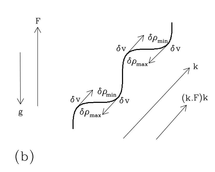
Figure 4: Geometry of radiation pressure force due to density and opacity fluctuations for (a) downward and (b) upward propagating hydrodynamic acoustic waves. Depending on whether the multiplier of the radiation pressure force is positive or negative, one direction is damped and the other is unstable, provided the radiation pressure force is large enough to overcome other forms of damping.

The destabilizing force density is ${\bf k}({\bf k}\cdot{\bf F})\delta\rho$ times a numerical factor depending on opacity derivatives that may be positive or negative. For the purposes of discussion, let us assume for the moment that it is positive. Figure 4(a) illustrates the geometry of this force acting on a downward propagating acoustic wave. In this case ${\bf k}({\bf k}\cdot{\bf F})\delta\rho$ is everywhere opposite to the velocity perturbation, and the wave is therefore damped. However, for an upward propagating wave, shown in Figure 4(b), the force is everywhere in phase with the velocity perturbation, and therefore amplifies the wave. If we had chosen the numerical factor depending on opacity derivatives to be negative, then it would have been the upward propagating wave that is damped and the downward propagating wave that is amplified.

It is also possible to consider the effects of the destabilizing force density in terms of whether it induces a net lag or lead between the total pressure and density perturbations in the sound wave. Once again, only one direction of propagation is destabilizing when viewed in this way.

Examination of the growth rate in equation (57) reveals that it is just the combination of opacity derivatives $\Theta_{\rho}+(\gamma-1)\Theta_{T{\rm g}}$ that determines the action of the force, not the full factor $[1+\Theta_{\rho}+(\gamma-1)\Theta_{T{\rm g}}]$ in equation (71). Pure Thomson scattering media are not unstable by this mechanism. To see why this is so, it is necessary to examine the equation of motion (71) more closely. Using the perturbed continuity equation (46) and regrouping, equation (71) may be rewritten as

$$\rho{\partial\delta{\bf v}\over\partial t} = -{i{\bf k}c_{\rm g}^{2}\rho\over\omega}\left({\bf k}\cdot\delta{\bf v}\right)-{\kappa_{\rm F}\over c}{\bf k}\left[{4E\over 3}\left({\omega\over k^{2}}\right)\right]\delta\rho-{\kappa_{\rm F}\over c}{\bf k}\left[{4Ec\omega_{\rm a}(\gamma-1)^{2}\over\kappa_{\rm F}\rho\omega}\right]\delta\rho$$ (72)

$$+ {\kappa_{\rm F}\over k^{2}c}{\bf k}\left({\bf k}\cdot{\bf F}\right)\left[\Theta_{\rho}+(\gamma-1)\Theta_{T{\rm g}}\right]\delta\rho$$

$$+ \left[{\kappa_{\rm F}\over k^{2}c}{\bf k}\left({\bf k}\cdot{\bf F}\right)\delta\rho-{{\bf k}\over\omega}\delta{\bf v}\cdot{\hbox{{\syvec\char 114\relax}}}p+{\bf g}\delta\rho\right]+{\cal O}(k^{-1})\delta\rho.$$

It is convenient to rewrite this equation in terms of the Lagrangian displacement ¸, where

$$\delta{\bf v}={\partial{\hbox{{\gkvec\char 24\relax}}}\over\partial t}=-i\omega{\hbox{{\gkvec\char 24\relax}}}.$$ (73)

Using the fact that to lowest order in $k^{-1}$, $\delta\rho=-i\rho{\bf k}\cdot{\hbox{{\gkvec\char 24\relax}}}$ from the continuity equation (46), we obtain

$${\partial^{2}{\hbox{{\gkvec\char 24\relax}}}\over\partial t^{2}} = -{\bf k}c_{\rm g}^{2}\left({\bf k}\cdot{\hbox{{\gkvec\char 24\relax}}}\right)$$ (74)

$$+ i({\bf k}\cdot{\hbox{{\gkvec\char 24\relax}}}){\bf k}{\kappa_{\rm F}\over c}\left\{{4E\over 3}\left({\omega\over k^{2}}\right)+{4Ec\omega_{\rm a}(\gamma-1)^{2}\over\kappa_{\rm F}\rho\omega}-{1\over k^{2}}({\bf k}\cdot{\bf F})\left[\Theta_{\rho}+(\gamma-1)\Theta_{T{\rm g}}\right]\right\}$$

$$- i\left[{\kappa_{\rm F}\over k^{2}c}{\bf k}\left({\bf k}\cdot{\bf F}\right)\left({\bf k}\cdot{\hbox{{\gkvec\char 24\relax}}}\right)-{1\over\rho}{\bf k}{\hbox{{\gkvec\char 24\relax}}}\cdot{\hbox{{\syvec\char 114\relax}}}p+{\bf g}\left({\bf k}\cdot{\hbox{{\gkvec\char 24\relax}}}\right)\right]+{\cal O}(k^{0})|{\hbox{{\gkvec\char 24\relax}}}|.$$

The destabilizing ${\bf k}\cdot{\bf F}$ term that would be present in Thomson scattering atmospheres competes with the equilibrium gravitational acceleration and gas pressure gradient in the last term in square brackets in equation (74). Figure 4 illustrates this by showing that the projection of ${\bf g}\delta\rho$ along the wave acts in the opposite direction to ${\bf k}\cdot{\bf F}{\bf k}\delta\rho$. Eliminating the gas pressure gradient using the hydrostatic equilibrium equation (21), the last term in square brackets in equation (74) may be written

$${\kappa_{\rm F}\over k^{2}c}{\bf k}\left({\bf k}\cdot{\bf F}\right)\left({\bf k}\cdot{\hbox{{\gkvec\char 24\relax}}}\right)-{\bf k}{\hbox{{\gkvec\char 24\relax}}}\cdot{\hbox{{\syvec\char 114\relax}}}p+{\bf g}\left({\bf k}\cdot{\hbox{{\gkvec\char 24\relax}}}\right)=-{\kappa_{\rm F}\over c}{\bf k}(\hat{\bf k}\times{\bf F})\cdot(\hat{\bf k}\times{\hbox{{\gkvec\char 24\relax}}})-{\hbox{{\gkvec\char 24\relax}}}\times({\bf k}\times{\bf g}).$$ (75)

Because hydrodynamic acoustic waves are longitudinal to lowest order in $k^{-1}$, ${\hbox{{\gkvec\char 24\relax}}}\propto{\bf k}$, and the term involving the flux vanishes. In addition, the second term does no work as it is perpendicular to the displacement. Hence these terms contribute nothing to the growth rate - the destabilizing radiation pressure force that would be present in a Thomson scattering medium is exactly cancelled due to the hydrostatic equilibrium of the unperturbed flow, at least for longitudinal waves. In the high-$k$ limit, the modes with density perturbations that can couple to the equilibrium radiation force are necessarily longitudinal. This is why gravity waves do not experience radiative driving in the short wavelength limit.

Taking the scalar product of equation (74) with the wave vector ${\bf k}$, we obtain

$${\partial^{2}\over\partial t^{2}}({\bf k}\cdot{\hbox{{\gkvec\char 24\relax}}}) = -k^{2}c_{\rm g}^{2}\left({\bf k}\cdot{\hbox{{\gkvec\char 24\relax}}}\right)+ik^{2}({\bf k}\cdot{\hbox{{\gkvec\char 24\relax}}}){\kappa_{\rm F}\over c}\Biggl{\{}{4E\over 3}\left({\omega\over k^{2}}\right)+{4Ec\omega_{\rm a}(\gamma-1)^{2}\over\kappa_{\rm F}\rho\omega}$$ (76)

$$- {1\over k^{2}}({\bf k}\cdot{\bf F})\left[\Theta_{\rho}+(\gamma-1)\Theta_{T{\rm g}}\right]\Biggr{\}}+{\cal O}(k)|{\hbox{{\gkvec\char 24\relax}}}|.$$

Replacing $\partial/\partial t$ with $-i\omega$, we immediately recover equation (57) for the mode frequency and growth rate.

We may repeat this procedure to better understand the instability in the limit where the gas and radiation exchange heat extremely rapidly. The gas and radiation temperatures are then locked together, so that

$$\delta T_{\rm g}=\delta T_{\rm r}\equiv\delta T={T\over 4E}\delta E=T\left({\delta p\over p}-{\delta\rho\over\rho}\right).$$ (77)

In this regime we must replace the separate gas and radiation energy equations with a single, combined energy equation which, when perturbed, gives

$$-i\omega\left({\delta p\over\gamma-1}+\delta E\right) = -{k^{2}c\over 3\kappa_{\rm F}\rho}\delta E-i\omega\left({c_{\rm g}^{2}\over\gamma-1}+3c_{\rm r}^{2}\right)\delta\rho-\rho T\delta{\bf v}\cdot{\hbox{{\syvec\char 114\relax}}}(S_{\rm g}+S_{\rm r})$$ (78)

$$+ i{\bf k}\cdot{\bf F}\left[(1+\Theta_{\rho}){\delta\rho\over\rho}+(\Theta_{T{\rm g}}+\Theta_{T{\rm r}}){\delta T\over T}\right].$$

Once again, equation (78) immediately implies that $\delta E\sim{\cal O}(k^{-1})\delta\rho$ for short wavelength acoustic waves. Rapid radiative diffusion smooths out both gas and radiation temperature fluctuations in this case. Equation (77) then implies that $\delta p=c_{\rm i}^{2}\delta\rho$ to lowest order, i.e. that the acoustic waves are isothermal in this limit. Equation (78) can then be solved for the radiation pressure perturbation,

$${\delta E\over 3}=-{i\kappa_{\rm F}\over c}\left(p+{4E\over 3}\right)\left({\omega\over k^{2}}\right)\delta\rho+{i\kappa_{\rm F}\over k^{2}c}({\bf k}\cdot{\bf F})(1+\Theta_{\rho})\delta\rho+{\cal O}(k^{-2})\delta\rho.$$ (79)

From equation (77), the gas pressure perturbation is given to the same order by

$$\delta p=c_{\rm i}^{2}\delta\rho-{i\kappa_{\rm F}\over c}\left(1+{3p\over 4E}\right)p\left({\omega\over k^{2}}\right)\delta\rho+{i\kappa_{\rm F}\over k^{2}c}\left({3p\over 4E}\right)({\bf k}\cdot{\bf F})(1+\Theta_{\rho})\delta\rho+{\cal O}(k^{-2})\delta\rho.$$ (80)

The first term on the right hand side of equation (79) and the second term on the right hand side of equation (80) are the damping terms due to radiative diffusion. The last terms in both equations are the potentially destabilizing terms from the equilibrium radiation flux acting on density and opacity fluctuations. Note that the opacity derivative with respect to temperature, $\Theta_{T{\rm g}}$, has been lost because the gas temperature is locked to the uniform radiation temperature. There is also no buoyancy response in the pressure perturbations to this order, as expected because of the suppression of gravity waves in this limit.

Using equations (79)-(80), the gas momentum equation (47) becomes

$$\rho{\partial\delta{\bf v}\over\partial t} = -i{\bf k}c_{\rm i}^{2}\delta\rho-{\kappa_{\rm F}\over c}{\bf k}\left(1+{3p\over 4E}\right)\left({4E\over 3}+p\right)\left({\omega\over k^{2}}\right)\delta\rho$$ (81)

$$+ {\kappa_{\rm F}\over k^{2}c}{\bf k}\left({\bf k}\cdot{\bf F}\right)\left(1+{3p\over 4E}\right)\left(1+\Theta_{\rho}\right)\delta\rho+{\bf g}\delta\rho+{\cal O}(k^{-1})\delta\rho.$$

Once again, the destabilizing force density term is proportional to ${\bf k}({\bf k}\cdot{\bf F})\delta\rho$, and the geometry of Figure 4 still applies. Repeating the same steps as before, we obtain

$${\partial^{2}{\hbox{{\gkvec\char 24\relax}}}\over\partial t^{2}} = -{\bf k}c_{\rm i}^{2}({\bf k}\cdot{\hbox{{\gkvec\char 24\relax}}})$$ (82)

$$+ i({\bf k}\cdot{\hbox{{\gkvec\char 24\relax}}}){\bf k}{\kappa_{\rm F}\over c}\left(1+{3p\over 4E}\right)\left[\left({4E\over 3}+p\right){\omega\over k^{2}}-{1\over k^{2}}({\bf k}\cdot{\bf F})\Theta_{\rho}\right]$$

$$- i\left[\left(1+{3p\over 4E}\right){\kappa_{\rm F}\over k^{2}c}{\bf k}({\bf k}\cdot{\bf F})({\bf k}\cdot{\hbox{{\gkvec\char 24\relax}}})-{\bf k}c_{\rm i}^{2}{\hbox{{\gkvec\char 24\relax}}}\cdot{\hbox{{\syvec\char 114\relax}}}\ln\rho+{\bf g}({\bf k}\cdot{\hbox{{\gkvec\char 24\relax}}})\right]+{\cal O}(k^{0})|{\hbox{{\gkvec\char 24\relax}}}|,$$

which should be compared with equation (74). The destabilizing ${\bf k}\cdot{\bf F}$ term that would remain in a pure Thomson scattering atmosphere again competes with other forces in the last term in square brackets. Using the equilibrium LTE condition (20), the hydrostatic equilibrium equation (21), and the radiative diffusion equation (23), the equilibrium density gradient is given by

$$c_{\rm i}^{2}{\hbox{{\syvec\char 114\relax}}}\ln\rho={\bf g}+\left(1+{3p\over 4E}\right){\kappa_{\rm F}\over c}{\bf F}.$$ (83)

The last term in square brackets in equation (82) is therefore

$$\left(1+{3p\over 4E}\right){\kappa_{\rm F}\over k^{2}c}{\bf k}({\bf k}\cdot{\bf F})({\bf k}\cdot{\hbox{{\gkvec\char 24\relax}}})-{\bf k}c_{\rm i}^{2}{\hbox{{\gkvec\char 24\relax}}}\cdot{\hbox{{\syvec\char 114\relax}}}\ln\rho+{\bf g}({\bf k}\cdot{\hbox{{\gkvec\char 24\relax}}})=-\left(1+{3p\over 4E}\right){\kappa_{\rm F}\over c}{\bf k}(\hat{\bf k}\times{\bf F})\cdot(\hat{\bf k}\times{\hbox{{\gkvec\char 24\relax}}})-{\hbox{{\gkvec\char 24\relax}}}\times({\bf k}\times{\bf g}).$$ (84)

Once again, these terms do not affect the growth rate for longitudinal waves. After taking the scalar product of equation (82) with ${\bf k}$, we finally obtain

$${\partial^{2}\over\partial t^{2}}\left({\bf k}\cdot{\hbox{{\gkvec\char 24\relax}}}\right) = -k^{2}c_{\rm i}^{2}\left({\bf k}\cdot{\hbox{{\gkvec\char 24\relax}}}\right)+ik^{2}({\bf k}\cdot{\hbox{{\gkvec\char 24\relax}}}){\kappa_{\rm F}\over c}\left(1+{3p\over 4E}\right)\Biggl{[}\left({4E\over 3}+p\right){\omega\over k^{2}}$$ (85)

$$- {1\over k^{2}}\left({\bf k}\cdot{\bf F}\right)\Theta_{\rho}\Biggr{]}+{\cal O}(k)|{\hbox{{\gkvec\char 24\relax}}}|,$$

from which we recover the growth rate (62).

4.1 Relation to the NAR Approximation

Gautschy & Glatzel (1990) have shown that strange modes are well-described by a so-called non-adiabatic reversible (NAR) approximation. Mathematically, this approximation reduces to taking the scalar product of the perturbed radiative diffusion equation (32) with ${\bf k}$, and then setting ${\bf k}\cdot\delta{\bf F}=0$. One also ignores the radiation energy equation (29). In addition, if the gas and radiation temperatures are locked together by rapid emission and absorption of photons, the gas energy equation (28) is also ignored. The perturbed radiation pressure is then given by

$$-ik^{2}{\delta E\over 3}={\kappa_{\rm F}\rho\over c}{\bf k}\cdot{\bf F}\left({\delta\rho\over\rho}+{\delta\kappa_{\rm F}\over\kappa_{\rm F}}\right).$$ (86)

This equation recovers our high $k$ expressions (70) and (79) for the perturbed radiation pressure, except that the NAR approximation cannot reproduce the radiation diffusion damping terms (as it neglects the radiation energy equation). Indeed, if we use equations (32), (70) and (79) to derive the perturbed radiative flux, we find

$$\delta{\bf F}=\cases{-3c_{\rm r}^{2}\left({\omega\over k^{2}}\right){\bf k}\delta\rho+\left[{{\bf k}({\bf k}\cdot{\bf F})\over k^{2}}-{\bf F}\right]\left[1+\Theta_{\rho}+(\gamma-1)\Theta_{T{\rm g}}\right]{\delta\rho\over\rho}+{\cal O}(k^{-1}){\delta\rho}&if $\delta T_{\rm r}\neq\delta T_{\rm g}$,\cr-(c_{\rm i}^{2}+3c_{\rm r}^{2})\left({\omega\over k^{2}}\right){\bf k}\delta\rho+\left[{{\bf k}({\bf k}\cdot{\bf F})\over k^{2}}-{\bf F}\right](1+\Theta_{\rho}){\delta\rho\over\rho}+{\cal O}(k^{-1}){\delta\rho}&if $\delta T_{\rm r}=\delta T_{\rm g}$.}$$ (87)

When unstable driving (the second term on the right hand sides) strongly dominates radiative diffusion damping (the first term on the right hand sides), the NAR approximation that ${\bf k}\cdot\delta{\bf F}=0$ is excellent.

By not invoking the NAR approximation, however, we are able to deduce the threshold criteria listed in Table 1 required for the unstable driving to exceed the damping by radiative diffusion. At the same time, we can also calculate the actual luminosity perturbation associated with the unstable wave.

5 MHD Instabilities in a Static Medium

We now extend the analysis of the previous section by including magnetic stresses. It turns out that magnetic fields widen the domain of the acoustic wave instabilities to include even pure Thomson scattering media. This is because magnetic tension endows acoustic waves with a mixed longitudinal/transverse character, except in the special cases of propagation purely along or perpendicular to the magnetic field.

5.1 Short Wavelength Limit

The dispersion relation (49) again factors easily in the short wavelength limit:

$$0 = \left[\omega^{2}-({\bf k}\cdot{\bf v}_{\rm A})^{2}\right]\left[\omega^{4}-\omega^{2}k^{2}(v_{\rm A}^{2}+c_{\rm g}^{2})+k^{2}c_{\rm g}^{2}({\bf k}\cdot{\bf v}_{\rm A})^{2}\right]$$ (88)

$$\times \left(\omega+{ick^{2}\over 3\kappa_{\rm F}\rho}\right)\left[\omega+{4i\omega_{\rm a}E(\gamma-1)\over\gamma p}\right].$$

From left to right, the factors correspond to Alfvén waves, fast and slow magnetosonic waves, the damped radiative diffusion mode, and a damped $\delta T_{\rm g}\neq\delta T_{\rm r}$ mode. The gravity waves of equation (54) have been lost because they are dominated by magnetic fields in this short wavelength limit, at least when ${\bf k}\cdot{\bf v}_{\rm A}\neq 0$, i.e. for wave vectors that are not orthogonal to the equilibrium magnetic field.

The first order corrections to the Alfvén modes vanish, so that $\omega=\pm{\bf k}\cdot{\bf v}_{\rm A}+{\cal O}(k^{-1})$. Because Alfvén waves are purely transverse and thus do not involve density fluctuations in this short wavelength limit, they do not couple to the radiation physics.

To the same order, the magnetosonic wave frequencies are given by

$$\omega = \pm kv_{\rm ph}-{i\kappa_{\rm F}\over 2cv_{\rm ph}}\left[{v_{\rm ph}^{2}-(\hat{\bf k}\cdot{\bf v}_{A})^{2}\over 2v_{\rm ph}^{2}-v_{\rm A}^{2}-c_{\rm g}^{2}}\right]\left\{{4Ev_{\rm ph}\over 3}+{4Ec\omega_{\rm a}(\gamma-1)^{2}\over\kappa_{\rm F}\rho v_{\rm ph}}\mp\left(\hat{\bf k}\cdot{\bf F}\right)\left[\Theta_{\rho}+(\gamma-1)\Theta_{T{\rm g}}\right]\right\}$$ (89)

$$\pm{i\kappa_{\rm F}\over 2cv_{\rm ph}(2v_{\rm ph}^{2}-v_{\rm A}^{2}-c_{\rm g}^{2})}(\hat{\bf k}\cdot{\bf v}_{\rm A})(\hat{\bf k}\times{\bf v}_{\rm A})\cdot(\hat{\bf k}\times{\bf F})+{\cal O}(k^{-1}),$$

where $v_{\rm ph}>0$ is the phase speed of the fast and slow magnetosonic waves, given by

$$v_{\rm ph}^{2}\equiv{1\over 2}\left\{v_{\rm A}^{2}+c_{\rm g}^{2}\pm\left[(v_{A}^{2}+c_{\rm g}^{2})^{2}-4(\hat{\bf k}\cdot{\bf v}_{\rm A})^{2}c_{\rm g}^{2}\right]^{1/2}\right\}.$$ (90)

Equation (89) bears a strong resemblance to its hydrodynamic counterpart (57). The gas sound speed $c_{\rm g}$ has been replaced by the phase velocity of the relevant magnetosonic wave $v_{\rm ph}$, and the “hydrodynamic” corrections to the mode frequency have been multiplied by a factor

$$\left({v_{\rm ph}^{2}-(\hat{\bf k}\cdot{\bf v}_{A})^{2}\over 2v_{\rm ph}^{2}-v_{\rm A}^{2}-c_{\rm g}^{2}}\right)\geq 0.$$ (91)

The last term in equation (89) is a new, destabilizing term that exists only in the presence of magnetic fields. As we discuss in more detail in section 6 below, its physical origin ultimately arises from the ability of magnetic stresses to support velocity perturbations that are not purely longitudinal, i.e. that are not parallel or antiparallel to the wave vector ${\bf k}$. Note that this term vanishes for wave vectors that are either parallel or perpendicular to the equilibrium magnetic field. In each of these cases the compressive magnetosonic wave is longitudinal.

In the rapid heat exchange ($\omega_{\rm a}\rightarrow\infty$) limit, one of the eight modes is lost for the same reason as in the hydrodynamic case, and the remaining seven modes factor in the short wavelength limit as

$$0 = \left[\omega^{2}-({\bf k}\cdot{\bf v}_{\rm A})^{2}\right]\left[\omega^{4}-\omega^{2}k^{2}(v_{\rm A}^{2}+c_{\rm i}^{2})+k^{2}c_{\rm i}^{2}({\bf k}\cdot{\bf v}_{\rm A})^{2}\right]$$ (92)

$$\times \left[\omega+{ick^{2}\over 3\kappa_{\rm F}\rho}\left({4(\gamma-1)E\over p+4(\gamma-1)E}\right)\right].$$

Once again, instabilities only occur in the fast and slow magnetosonic waves, whose frequencies are given to first order by

$$\omega = \pm kv_{\rm ph}-{i\kappa_{\rm F}\over 2cv_{\rm ph}}\left[{v_{\rm ph}^{2}-(\hat{\bf k}\cdot{\bf v}_{A})^{2}\over 2v_{\rm ph}^{2}-v_{\rm A}^{2}-c_{\rm i}^{2}}\right]\left(1+{3p\over 4E}\right)\left\{\left({4E\over 3}+p\right)v_{\rm ph}\mp\left(\hat{\bf k}\cdot{\bf F}\right)\Theta_{\rho}\right\}$$ (93)

$$\pm{i\kappa_{\rm F}\over 2cv_{\rm ph}(2v_{\rm ph}^{2}-v_{\rm A}^{2}-c_{\rm i}^{2})}\left(1+{3p\over 4E}\right)(\hat{\bf k}\cdot{\bf v}_{\rm A})(\hat{\bf k}\times{\bf v}_{\rm A})\cdot(\hat{\bf k}\times{\bf F})+{\cal O}(k^{-1}),$$

where $v_{\rm ph}$ is given by equation (90) with $c_{\rm g}$ replaced by the isothermal sound speed $c_{\rm i}$.

Equation (90) implies that $(2v_{\rm ph}^{2}-v_{\rm A}^{2}-c_{\rm g}^{2})$ is positive for fast modes and negative for slow modes. Hence if the last “magnetic” destabilizing term in equation (89), or (93), dominates the hydrodynamic terms, the unstable fast and slow waves will have opposite vector phase velocities. It is also easy to see that in this case the slow mode will always grow faster than the fast mode. However, if hydrodynamic driving (the opacity derivative terms in eqs. [89] and [93]) dominates magnetic driving, then whichever of the two modes has the larger density perturbation for a given velocity perturbation will be the one that grows fastest. If $v_{\rm A}^{2}\gg c_{\rm g}^{2}$, the slow mode grows faster, whereas if $v_{\rm A}^{2}\ll c_{\rm g}^{2}$, the fast mode grows faster.

5.2 Short Wavelength Limit With ${\bf k}\cdot{\bf v}_{\rm A}=0$: Recovery of Gravity Waves

If we consider wave vectors that are orthogonal to the equilibrium magnetic field, then the short wavelength limit recovers the fast magnetosonic modes, the radiative diffusion mode, and gives us a cubic equation describing coupled gravity and $\delta T_{\rm g}\neq\delta T_{\rm r}$ modes:

$$0 = (v_{\rm A}^{2}+c_{\rm g}^{2})\omega^{3}+{4i(\gamma-1)\omega_{\rm a}E\over p}(v_{\rm A}^{2}+c_{\rm i}^{2})\omega^{2}-\left[1-(\hat{\bf k}\cdot\hat{\bf z})^{2}\right]\left(c_{\rm g}^{2}N_{\rm g}^{2}+v_{\rm A}^{2}{\bf g}\cdot{\hbox{{\syvec\char 114\relax}}}\ln\rho\right)\omega$$ (94)

$$- \left[1-(\hat{\bf k}\cdot\hat{\bf z})^{2}\right]{4i(\gamma-1)\omega_{\rm a}E\over p}v_{\rm A}^{2}{\bf g}\cdot{\hbox{{\syvec\char 114\relax}}}\ln\rho.$$

The reason we recover gravity waves in this limit is that magnetic tension does not exist when ${\bf k}\cdot{\bf v}_{\rm A}=0$, and therefore no longer dominates buoyancy at short wavelengths. For weak thermal coupling between the gas and radiation, $\omega_{\rm a}\rightarrow 0$, the roots of this dispersion relation correspond to magnetically altered gravity waves in the gas,

$$\omega^{2}={1-(\hat{\bf k}\cdot\hat{\bf z})^{2}\over v_{\rm A}^{2}+c_{\rm g}^{2}}\left(c_{\rm g}^{2}N_{\rm g}^{2}+v_{\rm A}^{2}{\bf g}\cdot{\hbox{{\syvec\char 114\relax}}}\ln\rho\right),$$ (95)

and a mode

$$\omega\simeq-{4i(\gamma-1)\omega_{\rm a}E\over p}\left({v_{\rm A}^{2}{\bf g}\cdot{\hbox{{\syvec\char 114\relax}}}\ln\rho\over c_{\rm g}^{2}N_{\rm g}^{2}+v_{\rm A}^{2}{\bf g}\cdot{\hbox{{\syvec\char 114\relax}}}\ln\rho}\right).$$ (96)

In the rapid heat exchange limit, $\omega_{\rm a}\rightarrow\infty$, the last mode is lost and the gravity waves depend only on the vertical density profile,

$$\omega^{2}={1-(\hat{\bf k}\cdot\hat{\bf z})^{2}\over v_{\rm A}^{2}+c_{\rm i}^{2}}v_{\rm A}^{2}{\bf g}\cdot{\hbox{{\syvec\char 114\relax}}}\ln\rho.$$ (97)

5.3 The Limit of Zero Gas Pressure: Photon Bubbles

Just as in the hydrodynamic case, a number of authors (Arons 1992, Gammie 1998) have investigated the slow mode instability in the limit of zero gas pressure. Because the phase speed of the slow mode then vanishes, the instability then loses its obvious connection to this mode.

Setting $p=0=c_{\rm g}^{2}$ in the dispersion relation (49), and then assuming $\omega\propto k^{1/2}$ as $k\rightarrow\infty$, we find two modes with

$$\omega^{2} = {i\kappa_{\rm F}\over cv_{\rm A}^{2}}{\bf k}\cdot{\bf v}_{\rm A}\left[(\hat{\bf k}\cdot{\bf v}_{\rm A})(\hat{\bf k}\cdot{\bf F})\Theta_{\rho}-(\hat{\bf k}\times{\bf v}_{\rm A})\cdot(\hat{\bf k}\times{\bf F})\right]$$ (98)

$$= -{i\over v_{\rm A}^{2}}{\bf k}\cdot{\bf v}_{\rm A}\left[(\hat{\bf k}\cdot{\bf v}_{\rm A})(\hat{\bf k}\cdot{\bf g})\Theta_{\rho}-(\hat{\bf k}\times{\bf v}_{\rm A})\cdot(\hat{\bf k}\times{\bf g})\right].$$

Just as in the hydrodynamic case [eq. (64)], equation (98) can be obtained from the thermally locked slow mode frequency in equation (93) by first squaring the frequency and then taking the limit of zero gas pressure. Again, we lose the damping terms in this limit, which determine the instability threshold for short wavelength modes.

If we first assume negligible thermal coupling between the gas and radiation, and then take the limit of zero gas pressure, we obtain instead

$$\omega^{2} = {i\kappa_{\rm F}\over cv_{\rm A}^{2}}{\bf k}\cdot{\bf v}_{\rm A}\left\{(\hat{\bf k}\cdot{\bf v}_{\rm A})(\hat{\bf k}\cdot{\bf F})[\Theta_{\rho}+(\gamma-1)\Theta_{T{\rm g}}]-(\hat{\bf k}\times{\bf v}_{\rm A})\cdot(\hat{\bf k}\times{\bf F})\right\}$$ (99)

$$= -{i\over v_{\rm A}^{2}}{\bf k}\cdot{\bf v}_{\rm A}\left\{(\hat{\bf k}\cdot{\bf v}_{\rm A})(\hat{\bf k}\cdot{\bf g})[\Theta_{\rho}+(\gamma-1)\Theta_{T{\rm g}}]-(\hat{\bf k}\times{\bf v}_{\rm A})\cdot(\hat{\bf k}\times{\bf g})\right\}.$$

In a Thomson scattering medium, $\Theta_{\rho}=\Theta_{T{\rm g}}=0$, and equations (98)-(99) are identical to the photon bubble dispersion relation derived by Gammie [1998, his eq. (41)]. As noted both by Gammie (1998) and BS01, this growth rate only applies for wavelengths longer than the gas pressure scale height $\sim c_{\rm g}^{2}/g$. Unless this wavelength scale is optically thin, in which case our diffusion-based analysis breaks down, then the maximal growth rate occurs at wavelengths shorter than the gas pressure scale height, and is given by equations (89) or (93).

There has been some confusion as to how Gammie’s (1998) work on photon bubbles relates to the original analysis performed by Arons (1992), who also assumed a pure Thomson scattering medium with zero gas pressure. Gammie’s (1998) result can in fact be obtained as the short wavelength limit of Arons’ (1992) dispersion relation [his eq. (33)], at least within the latter’s assumed vertical magnetic field geometry. Arons’ (1992) numerical growth rates all climb toward higher wavenumber, and must therefore eventually recover the $k^{1/2}$ dependence of equation (98), provided the medium remains optically thick at these short wavelengths. Arons (1992) was mainly interested in long wavelengths where radiation diffusion was slow compared to the (radiation) acoustic wave period. Gammie (1998), on the other hand, was working in the rapid diffusion regime at shorter wavelengths.

5.4 Numerical Results

Table 2 summarizes the instability thresholds, growth rates, and characteristic wavenumbers for the magnetoacoustic wave instabilities in media with a variety of ratios of magnetic, gas thermal, and radiation energy densities. We have assumed a pure Thomson scattering equilibrium throughout this table, so that the hydrodynamic driving forces that we addressed in sections 3 and 4 vanish, and only the magnetically-based driving remains.

Figure 5 illustrates growth rates of unstable slow waves for small values of the thermal coupling frequency $\omega_{\rm th}$ for a radiation pressure dominated equilibrium, for which the asymptotic high wavenumber growth rate is accurately given by equation (89). Just as in the hydrodynamic case, the short wavelength growth rate declines with increasing thermal coupling. This continues until $\omega_{\rm th}$ exceeds $g/c_{\rm g}$, beyond which the gas and radiation temperatures are effectively locked and the waves reach unstable asymptotic growth rates given by equation (93), as shown in Figure 6.

Just as in the hydrodynamic case, the unstable growth rate for high thermal coupling only extends over a finite range of wavenumbers. Above a critical cutoff wavenumber, the waves again become damped. After numerical experimentation, we deduced the physical dependencies of these cutoff wavenumbers, and they are listed in Table 2. Figure 7 illustrates the accuracy of these formulas in two specific cases, one with $v_{\rm A}>c_{\rm g}$ and one with $v_{\rm A}<c_{\rm g}$.

6 Physics of the MHD Wave Instabilities

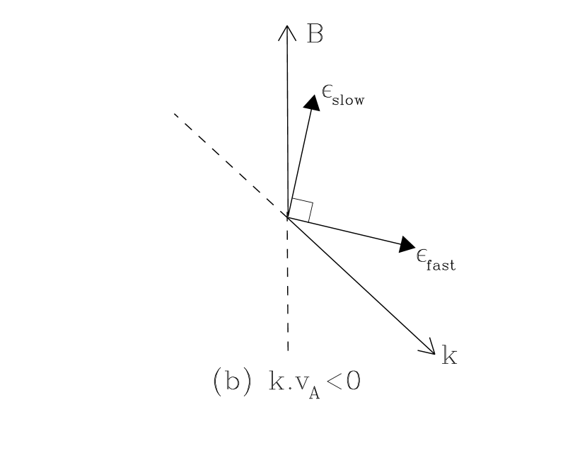
Figure 8: Polarizations of the fast and slow magnetosonic modes. All vectors shown lie in the plane of the page.

The magnetoacoustic wave instabilities are much more robust than their hydrodynamic counterparts, and in particular they survive unscathed even in pure Thomson scattering media. In order to see how this arises physically, we repeat the analysis of section 4 here to re-examine the competing forces acting on a parcel of gas in the wave. There are now two relevant waves that possess density fluctuations: the fast and slow magnetosonic waves. For reference, their polarizations are shown in Figure 8.

Using equation (48) to eliminate the magnetic field perturbation, and equations (69)-(70) to eliminate the total pressure perturbation, the perturbed gas momentum equation (47) may be written in the high wavenumber limit as

$${\partial^{2}{\hbox{{\gkvec\char 24\relax}}}\over\partial t^{2}} = -({\bf k}\cdot{\bf v}_{\rm A})^{2}{\hbox{{\gkvec\char 24\relax}}}+({\bf k}\cdot{\hbox{{\gkvec\char 24\relax}}})({\bf k}\cdot{\bf v}_{\rm A}){\bf v}_{\rm A}+({\bf k}\times{\bf v}_{\rm A})\cdot({\bf v}_{\rm A}\times{\hbox{{\gkvec\char 24\relax}}}){\bf k}-{\bf k}c_{\rm g}^{2}({\bf k}\cdot{\hbox{{\gkvec\char 24\relax}}})$$ (100)

$$+ i({\bf k}\cdot{\hbox{{\gkvec\char 24\relax}}}){\bf k}{\kappa_{\rm F}\over c}\left\{{4E\over 3}\left({\omega\over k^{2}}\right)+{4Ec\omega_{\rm a}(\gamma-1)^{2}\over\kappa_{\rm F}\rho\omega}-{1\over k^{2}}({\bf k}\cdot{\bf F})\left[\Theta_{\rho}+(\gamma-1)\Theta_{T{\rm g}}\right]\right\}$$

$$+ i\left[{\kappa_{\rm F}\over c}{\bf k}(\hat{\bf k}\times{\bf F})\cdot(\hat{\bf k}\times{\hbox{{\gkvec\char 24\relax}}})+{\hbox{{\gkvec\char 24\relax}}}\times({\bf k}\times{\bf g})\right]+{\cal O}(k^{0})|{\hbox{{\gkvec\char 24\relax}}}|.$$

Apart from the additional magnetic terms, this equation is of course identical to its hydrodynamic counterpart, equation (74), which we discussed above in section 4. There we found that the last term in square brackets did not affect the growth rate. This continues to be true for the piece of this term that involves the gravitational acceleration ${\bf g}$, as this piece does no work. However the first piece that involves the radiative flux now can play a role because magnetosonic waves are, in general, not longitudinal due to the effects of magnetic tension.

In the short wavelength limit, the fast and slow magnetosonic modes described by equation (100) are polarized in the plane of ${\bf k}$ and ${\bf v}_{\rm A}$, and their Lagrangian displacements may be written as

$${\hbox{{\gkvec\char 24\relax}}}=[v_{\rm ph}^{2}{\bf k}-({\bf k}\cdot{\bf v}_{\rm A}){\bf v}_{\rm A}]\psi\equiv{\hbox{{\gkvec\char 15\relax}}}\psi,$$ (101)

where $\psi$ is some complex scalar amplitude. Taking the scalar product of equation (100) with the polarization vector ffl, we obtain

$${\partial^{2}\over\partial t^{2}}({\hbox{{\gkvec\char 15\relax}}\cdot\hbox{{\gkvec\char 24\relax}}}) = -k^{2}v_{\rm ph}^{2}({\hbox{{\gkvec\char 15\relax}}\cdot\hbox{{\gkvec\char 24\relax}}})$$ (102)

$$+ ik^{2}[v_{\rm ph}^{2}-(\hat{\bf k}\cdot{\bf v}_{\rm A})^{2}]({\bf k}\cdot{\hbox{{\gkvec\char 24\relax}}}){\kappa_{\rm F}\over c}\Biggl{\{}{4E\over 3}\left({\omega\over k^{2}}\right)+{4Ec\omega_{\rm a}(\gamma-1)^{2}\over\kappa_{\rm F}\rho\omega}$$

$$- {1\over k^{2}}({\bf k}\cdot{\bf F})\left[\Theta_{\rho}+(\gamma-1)\Theta_{T{\rm g}}\right]\Biggr{\}}-i{\kappa_{\rm F}\over c}({\bf k}\cdot{\bf v}_{\rm A})({\bf k}\times{\bf v}_{\rm A})\cdot({\bf k}\times{\bf F})({\bf k}\cdot{\hbox{{\gkvec\char 24\relax}}}),$$

where, in the last term, we have used the fact that $({\bf k}\cdot{\hbox{{\gkvec\char 15\relax}}})({\bf k}\times{\hbox{{\gkvec\char 24\relax}}})=({\bf k}\cdot{\hbox{{\gkvec\char 24\relax}}})({\bf k}\times{\hbox{{\gkvec\char 15\relax}}})$. The expression for the growth rate, equation (89), now follows immediately from equation (102) and the fact that, to lowest order in $k^{-1}$,

$${{\bf k}\cdot{\hbox{{\gkvec\char 24\relax}}}\over{\hbox{{\gkvec\char 15\relax}}}\cdot{\hbox{{\gkvec\char 24\relax}}}}={1\over 2v_{\rm ph}^{2}-c_{\rm g}^{2}-v_{\rm A}^{2}}.$$ (103)

As illustrated in Figure 8, the polarizations of the fast and slow waves for fixed ${\bf k}$ are orthogonal, and this normalized projection of ¸ onto ${\bf k}$ therefore always has opposite signs for the two modes. Hence the unstable fast and slow modes propagate in different directions if the magnetic driving term dominates over the hydrodynamic terms.

To understand the physics of the MHD driving further, consider again the relevant force density ($\rho$ times the second to last term in equation [100]), which can be written as

$$i{\kappa_{\rm F}\rho\over c}{\bf k}(\hat{\bf k}\times{\bf F})\cdot(\hat{\bf k}\times{\hbox{{\gkvec\char 24\relax}}})=-i{\kappa_{\rm F}\rho\over c}{\bf k}\left[(\hat{\bf k}\cdot{\hbox{{\gkvec\char 24\relax}}})(\hat{\bf k}\cdot{\bf F})-({\hbox{{\gkvec\char 24\relax}}}\cdot{\bf F})\right].$$ (104)

MHD driving results fundamentally from a breakdown in cancellation of the two force densities on the right hand side of this equation, whenever the waves are not longitudinal. The first, $(\kappa_{\rm F}/c)\hat{\bf k}(\hat{\bf k}\cdot{\bf F})\delta\rho$, is the driving force based on density, not opacity, fluctuations that we illustrated in Figure 4. The second arises from a change in the radiation pressure along a fluid displacement, and is $i(\kappa_{\rm F}\rho/c){\bf k}({\hbox{{\gkvec\char 24\relax}}}\cdot{\bf F})$. If we ignore the radiation diffusion damping and opacity fluctuations in equation (70), these two force densities simply combine to give the negative gradient of the Lagrangian perturbation in radiation pressure $\Delta E/3$,

$$i{\kappa_{\rm F}\rho\over c}{\bf k}(\hat{\bf k}\times{\bf F})\cdot(\hat{\bf k}\times{\hbox{{\gkvec\char 24\relax}}})=-{\hbox{{\syvec\char 114\relax}}}\left({1\over 3}\Delta E\right)=-{\hbox{{\syvec\char 114\relax}}}\left({\delta E\over 3}+{{\hbox{{\gkvec\char 24\relax}}}\cdot{\hbox{{\syvec\char 114\relax}}}E\over 3}\right).$$ (105)

For any purely longitudinal wave (¸ and ${\bf k}$ parallel), the two force densities exactly cancel, and the Lagrangian radiation pressure perturbation then vanishes (again ignoring radiation diffusion damping and opacity fluctuations). For an MHD wave with fixed density perturbation $\delta\rho$ and fixed ${\bf k}$, magnetic tension can alter the direction of ¸ off of ${\bf k}$, provided propagation is neither along or perpendicular to the field. Spatial gradients in the flow (which determine the radiative heat flow) are no longer parallel to fluid displacements. The second force density on the right hand side of equation (104) will now be greater or less than the first, depending on the type of MHD wave (slow or fast) and the propagation direction. Note that the two force densities also cancel for vertical propagation.

The physics is very similar in the case where gas and radiation exchange heat rapidly. The perturbed gas momentum equation is then

$${\partial^{2}{\hbox{{\gkvec\char 24\relax}}}\over\partial t^{2}} = -({\bf k}\cdot{\bf v}_{\rm A})^{2}{\hbox{{\gkvec\char 24\relax}}}+({\bf k}\cdot{\hbox{{\gkvec\char 24\relax}}})({\bf k}\cdot{\bf v}_{\rm A}){\bf v}_{\rm A}+({\bf k}\times{\bf v}_{\rm A})\cdot({\bf v}_{\rm A}\times{\hbox{{\gkvec\char 24\relax}}}){\bf k}-{\bf k}c_{\rm i}^{2}({\bf k}\cdot{\hbox{{\gkvec\char 24\relax}}})$$ (106)

$$+ i({\bf k}\cdot{\hbox{{\gkvec\char 24\relax}}}){\bf k}{\kappa_{\rm F}\over c}\left(1+{3p\over 4E}\right)\left[\left({4E\over 3}+p\right){\omega\over k^{2}}-{1\over k^{2}}({\bf k}\cdot{\bf F})\Theta_{\rho}\right]$$

$$+ i\left[\left(1+{3p\over 4E}\right){\kappa_{\rm F}\over c}{\bf k}(\hat{\bf k}\times{\bf F})\cdot(\hat{\bf k}\times{\hbox{{\gkvec\char 24\relax}}})+{\hbox{{\gkvec\char 24\relax}}}\times({\bf k}\times{\bf g})\right]+{\cal O}(k^{0})|{\hbox{{\gkvec\char 24\relax}}}|.$$

Taking the scalar product of this equation with ffl, we obtain

$${\partial^{2}\over\partial t^{2}}({\hbox{{\gkvec\char 15\relax}}\cdot\hbox{{\gkvec\char 24\relax}}}) = -k^{2}v_{\rm ph}^{2}({\hbox{{\gkvec\char 15\relax}}\cdot\hbox{{\gkvec\char 24\relax}}})$$ (107)

$$+ ik^{2}[v_{\rm ph}^{2}-(\hat{\bf k}\cdot{\bf v}_{\rm A})^{2}]({\bf k}\cdot{\hbox{{\gkvec\char 24\relax}}}){\kappa_{\rm F}\over c}\left(1+{3p\over 4E}\right)\Biggl{[}\left({4E\over 3}+p\right){\omega\over k^{2}}$$

$$- {1\over k^{2}}({\bf k}\cdot{\bf F})\Theta_{\rho}\Biggr{]}-i\left(1+{3p\over 4E}\right){\kappa_{\rm F}\over c}({\bf k}\cdot{\bf v}_{\rm A})({\bf k}\times{\bf v}_{\rm A})\cdot({\bf k}\times{\bf F})({\bf k}\cdot{\hbox{{\gkvec\char 24\relax}}}).$$

With the help of equation (103) with $c_{\rm g}$ replaced by the isothermal sound speed $c_{\rm i}$, this now gives us the growth rate of equation (93).

We have extended Hearn’s (1972) hydrodynamic acoustic wave analysis of optically thin media to the magnetosonic wave instabilities, and have found that the extra magnetic piece of the instability vanishes completely in this regime. Physically, this is easy to understand. In the limit of vanishing optical depth, the dynamics of the radiation field can be ignored, and the equilibrium flux ${\bf F}$ merely acts to globally reduce the equilibrium gravitational acceleration ${\bf g}$ to ${\bf g}_{\rm eff}={\bf g}-\kappa_{\rm F}{\bf F}/c$. Hence, apart from the hydrodynamic driving terms that are proportional to logarithmic derivatives of $\kappa_{\rm F}$, the radiation flux enters the gas momentum equation only through a ${\hbox{{\gkvec\char 24\relax}}}\times({\bf k}\times{\bf g}_{\rm eff})$ term [the last term in equations (100) and (106)]. This term performs no work. Presumably, there will still be some level of instability in media with optical depths $\mathrel{\hbox to0.0pt{\lower 3.0pt\hbox{$\mathchar 536\relax$}\hss}\raise 2.0pt\hbox{$\mathchar 316\relax$}}1$, but an analysis of this situation is beyond the scope of the present paper.

7 Astrophysical Applications

We intend to investigate applications of the theory presented in this paper to particular astrophysical phenomena in future work. For now, we limit ourselves to a brief discussion of how these instabilities might manifest themselves in accretion disks and stars.

7.1 Accretion Disks

A number of authors have considered applications of strange modes (Glatzel & Mehren 1996, Mehren-Baehr & Glatzel 1999) and magnetic photon bubbles or magnetoacoustic waves (Gammie 1998; BS01; Begelman 2001, 2002) to radiation pressure dominated accretion disks around black holes.

The gas temperature is probably reasonably well-locked to the radiation temperature in standard accretion disk models. For stellar mass black holes, the most important atomic absorption opacity is bremsstrahlung, for which the Planck mean opacity is given in cgs units by

$$\kappa_{\rm P}\simeq 2.2\times 10^{24}\bar{g}_{\rm P}\rho T_{\rm g}^{-7/2},$$ (108)

where

$$\bar{g}_{\rm P}\equiv{h\over k_{\rm B}T_{\rm g}}\int_{0}^{\infty}d\nu\bar{g}_{\rm ff}e^{-h\nu/k_{\rm B}T_{\rm g}}$$ (109)

is an appropriate frequency-averaged Gaunt factor (Rybicki & Lightman 1979). Equation (108) gives a lower limit to the Planck mean opacity, which should also include bound-free and bound-bound contributions. These contributions are generally more important for the cooler disks thought to exist around supermassive black holes in active galactic nuclei.

By approximating $\bar{g}_{\rm ff}$ to be nearly constant inside the frequency integrals, it is also straightforward to show that for bremsstrahlung,

$$1+{1\over 4}{\partial\ln\kappa_{\rm J}\over\partial\ln T_{\rm r}}\simeq{\pi^{2}\over 6}\simeq 1.6.$$ (110)

For concreteness, consider a standard Shakura & Sunyaev (1973) disk model in which the anomalous stress is $\alpha$ times the total pressure. Using equations (30) and (66), the thermal coupling frequency due to bremsstrahlung is

$$\omega_{\rm th,bremss} \equiv \kappa_{\rm P}\rho c\left(1+{1\over 4}{\partial\ln\kappa_{\rm J}\over\partial\ln T_{\rm r}}\right)\left[{4(\gamma-1)E\over p}\right]$$ (111)

$$\simeq 3\times 10^{4}{\rm rad\,s}^{-1}\bar{g}_{\rm P}\eta^{2}\alpha^{-7/8}\left({M\over{\rm M}_{\odot}}\right)^{-7/8}\left({L\over L_{\rm Edd}}\right)^{-2}\left({r\over r_{\rm g}}\right)^{27/16}.$$

Here $L$ is the disk luminosity, $L_{\rm Edd}$ is the (Thomson scattering) Eddington luminosity, $M$ is the black hole mass, $\eta\equiv L/(\dot{M}c^{2})$ is the disk radiative efficiency, $r$ is the radius of the particular point of interest in the disk, and $r_{\rm g}\equiv GM/c^{2}$ is the gravitational radius of the black hole. We have neglected all relativistic correction factors in the disk model. The particular numerical value of the thermal coupling frequency in equation (111) assumes vertically averaged, disk interior quantities.

The corresponding thermal coupling frequency due to Compton scattering is

$$\omega_{\rm th,Comp}\equiv\kappa_{\rm T}\rho c\left({k_{\rm B}T\over m_{\rm e}c^{2}}\right)\left[{4(\gamma-1)E\over p}\right]\simeq 2\times 10^{9}{\rm rad\,s}^{-1}\alpha^{-1}\left({M\over{\rm M}_{\odot}}\right)^{-1}\left({r\over r_{\rm g}}\right)^{-3/2}.$$ (112)

Comparing equations (111) and (112), we see that Compton scattering generally dominates the thermal coupling of gas and radiation in the inner regions of the disk, while bremsstrahlung becomes more important further out, at least in the disk interior for this class of models. For hydrodynamic acoustic waves, the requirement that the gas and radiation temperatures be locked in the wave is that $\omega_{\rm th}$ exceed the sound wave frequency on scales of order the gas scale height $c_{\rm g}^{2}/g$, i.e. that $\omega_{\rm th}c_{\rm g}/g\mathrel{\hbox to0.0pt{\lower 3.0pt\hbox{$\mathchar 536\relax$}\hss}\raise 2.0pt\hbox{$\mathchar 318\relax$}}1$. For standard Shakura & Sunyaev (1973) models,

$$\omega_{\rm th,bremss}{c_{\rm g}\over g}\sim 4\times 10^{-4}\bar{g}_{\rm P}\eta^{3}\alpha^{-1}\left({L\over L_{\rm Edd}}\right)^{-3}\left({r\over r_{\rm g}}\right)^{9/2}$$ (113)

and

$$\omega_{\rm th,Comp}{c_{\rm g}\over g}\sim 3\times 10^{1}\eta\alpha^{-9/8}\left({M\over{\rm M}_{\odot}}\right)^{-1/8}\left({L\over L_{\rm Edd}}\right)^{-1}\left({r\over r_{\rm g}}\right)^{21/16}.$$ (114)

Hence while bremsstrahlung may be unable to ensure tight thermal coupling between the gas and the radiation in the innermost radii, Compton scattering is easily adequate. We stress, however, that these estimates are very uncertain as they do not properly take into account the vertical stratification in the disk. In particular, we have assumed a gravitational acceleration appropriate at the disk scale height but a temperature appropriate to the disk midplane. Because $\omega_{\rm th,Comp}c_{\rm g}/g\propto T^{3/2}$, it could be that in regions near the disk photosphere, the gas temperature may not be able to track the radiation temperature.

If the disk is treated hydrodynamically, then unstable acoustic wave growth rates are likely to be much slower than the dynamical frequency in the innermost parts of the disk because Thomson scattering dominates the Rosseland mean opacity. From Table 1, the maximum growth rate for hydrodynamic instabilities is roughly given by

$$\Theta_{\rho}{g\over c_{\rm g}} \sim \frac{g}{c_{\rm r}}\frac{c_{\rm r}}{c_{\rm g}}\frac{\kappa_{\rm a}}{\kappa_{\rm T}}\sim\Omega\frac{c_{\rm r}}{c_{\rm g}}\frac{\kappa_{\rm a}}{\kappa_{\rm T}}$$ (115)

$$\sim 3\times 10^{-5}\Omega\bar{g}_{\rm P}\eta\left({L\over L_{\rm Edd}}\right)^{-1}\left({r\over r_{\rm g}}\right)^{3/2}$$

for a radiation pressure supported disk with $\kappa_{a}\sim\kappa_{\rm P}$.

For example, Glatzel & Mehren (1996) found that a class of global strange mode instabilities was present at 25 km radii in accretion disk models around 1 ${\rm M}_{\odot}$ black holes with accretion rates of $10^{-9}$ ${\rm M}_{\odot}$ yr^-1. Our estimate (115) then gives a growth rate $\sim 5\times 10^{-3}\Omega$, in remarkable agreement with their calculated value $\sim 3\times 10^{-3}\Omega$. Mehren-Baehr & Glatzel (1999) also note that this class of modes has growth rates that decline as the ratio of gas pressure to radiation pressure increases, which is also in agreement with our estimate (115). In addition to these “hot” instabilities, Glatzel & Mehren (1996) and Mehren-Baehr & Glatzel (1999) found a class of unstable modes in colder regions of disk models where gas pressure was substantial. They found that these modes required the presence of a vertical opacity peak due to helium or hydrogen ionization, but that these modes also satisfied the NAR approximation and were therefore likely to be related to strange modes. We speculate that these modes are related to the local, WKB driving we find in the gas-pressure dominated case. Radiation pressure support is not essential for strange modes provided the gas and radiation temperatures are locked, as these authors implicitly assumed in their analysis.

It is almost certainly true, however, that the presence of magnetic fields cannot be neglected in these flows, and these allow in principle much faster growth rates through the slow mode instability (Gammie 1998, BS01). From Table 2, the maximum growth rate in this case is $\sim\Omega(c_{\rm r}/c_{\rm g}){\rm min}[1,(v_{\rm A}/c_{\rm g})]$, which can be much faster than the orbital frequency in the radiation pressure dominated inner regions. The characteristic length scale of the instability is given by the reciprocal of the turnover wavenumber, which is the gas scale height. Again in the radiation pressure dominated inner regions, this is smaller than the disk scale height by the ratio of the gas to radiation pressure. It is far from clear how this instability might, if at all, manifest itself in the presence of MRI turbulence. The MRI acts on longer time scales (the orbital time), and possibly length scales as well, and this separation of scales between the two instabilities suggests that they might both be simultaneously present. Numerical simulations of vertically stratified, radiating shear flows will be required to address this question.

7.2 Stellar Envelopes on the Main Sequence

Except possibly for short wavelength acoustic waves near the stellar photosphere, the gas and radiation temperatures are tightly coupled together in main sequence stellar envelopes. Thermal locking at the turnover wavenumber $\sim g/c_{\rm i}^{2}$ requires $\omega_{\rm th}\mathrel{\hbox to0.0pt{\lower 3.0pt\hbox{$\mathchar 536\relax$}\hss}\raise 2.0pt\hbox{$\mathchar 318\relax$}}g/c_{\rm i}$. For gas pressure supported envelopes, for example, this translates to the requirement that

$$\left(\frac{L}{{\rm L}_{\odot}}\right)\left(\frac{M}{{\rm M}_{\odot}}\right)^{-1}\left(\frac{\kappa_{F}\kappa_{\rm a}}{\kappa_{T}^{2}}\right)\left(\frac{\rho}{10^{-7}{\rm g\,cm}^{-3}}\right)\left(\frac{2\pi c_{\rm i}/g}{3{\rm minutes}}\right)^{-1}\mathrel{\hbox to0.0pt{\lower 3.0pt\hbox{$\mathchar 536\relax$}\hss}\raise 2.0pt\hbox{$\mathchar 318\relax$}}1,$$ (116)

which, given realistic envelope opacities, is usually satisfied.

From Table 1, if the gas and radiation temperatures are locked together, then the vertical radiative flux will destabilize short wavelength hydrodynamic acoustic waves in a radiation pressure dominated stellar envelope if $F\Theta_{\rho}\mathrel{\hbox to0.0pt{\lower 3.0pt\hbox{$\mathchar 536\relax$}\hss}\raise 2.0pt\hbox{$\mathchar 318\relax$}}Ec_{i}$. It is convenient to express this in terms of the flux mean (Rosseland) optical depth $\tau_{\rm F}$ of the particular envelope layer in question. Radiative diffusion implies that $F\sim Ec/\tau_{\rm F}$, so that short wavelength acoustic waves will be unstable in a radiation pressure dominated stellar envelope for all layers with optical depths satisfying

$$\tau_{\rm F}\mathrel{\hbox to0.0pt{\lower 3.0pt\hbox{$\mathchar 536\relax$}\hss}\raise 2.0pt\hbox{$\mathchar 316\relax$}}\left({c\over c_{\rm i}}\right)\Theta_{\rho}.$$ (117)

This can also be written as

$$\Theta_{\rho}\mathrel{\hbox to0.0pt{\lower 3.0pt\hbox{$\mathchar 536\relax$}\hss}\raise 2.0pt\hbox{$\mathchar 318\relax$}}3\times 10^{-5}\left({c_{\rm i}\over 10{\rm km\,s}^{-1}}\right)\tau_{\rm F}.$$ (118)

In a gas pressure supported stellar envelope, the instability criterion in Table 1 can be written in a similar fashion,

$$\tau_{\rm F}\mathrel{\hbox to0.0pt{\lower 3.0pt\hbox{$\mathchar 536\relax$}\hss}\raise 2.0pt\hbox{$\mathchar 316\relax$}}\left({c\over c_{\rm i}}\right)\left({E\over p}\right)\Theta_{\rho}.$$ (119)

Now, $p/E\sim L_{\rm Edd}/L$ if gas pressure dominates radiation pressure, where $L_{\rm Edd}$ is the Eddington luminosity appropriate for the Rosseland mean opacity $\kappa_{\rm F}$. Hence the instability criterion (119) may be rewritten as

$$\Theta_{\rho}\mathrel{\hbox to0.0pt{\lower 3.0pt\hbox{$\mathchar 536\relax$}\hss}\raise 2.0pt\hbox{$\mathchar 318\relax$}}3\times 10^{-5}\frac{L_{\rm Edd}}{L}\left(\frac{c_{i}}{10\,{\rm km\,s^{-1}}}\right)\tau_{\rm F}.$$ (120)

This equation strongly suggests that even in gas pressure supported envelopes on the mid- to upper main sequence, acoustic waves may be unstable and strange modes might exist.

We stress that we have only performed a local analysis of the stability of propagating waves in this paper. A demonstration that such waves are amplified by the background radiative flux does not necessarily imply that global compressive modes of the star will be unstable. This is because such modes can in general be viewed as superpositions of WKB waves propagating in different directions and, as we have seen, while one propagation direction may be driven, the other may very well be damped. Our instability criteria are therefore necessary, but not sufficient when it comes to global standing waves of the star. Note that the radiative driving becomes most important at lower optical depths, and it is also important to point out that we have not included the effects of turbulent damping associated with outer convection zones, when they exist.

Most main sequence stellar envelopes probably contain rather weak magnetic fields, and therefore the hydrodynamic driving that we have discussed so far is probably of greatest importance. There are exceptions, however, where MHD effects might play a role. In some chemically peculiar A and B-stars, for example, highly ordered, roughly dipolar magnetic fields of order 1 kG have been measured (e.g. Landstreet 1992). The MHD driving that we discussed in sections 5 and 6 above could produce instabilities in the upper layers of such stars, and magnetic effects will almost certainly alter the hydrodynamic driving. A particular case in point is that of roAp stars, which exhibit high order $p$-mode oscillations with low angular momentum quantum number $\ell$, largely confined to the poles of a dipole magnetic field (e.g. Kurtz 1990). Consider the possibility that hydrodynamic driving due to a large opacity variation dominates magnetic driving, but in the surface layers where the magnetic energy density dominates the gas pressure. From equation (90), the phase speed of slow modes in this case is $\simeq|\hat{\bf k}\cdot{\bf v}_{\rm A}/v_{\rm A}|c_{\rm i}$, assuming the gas and radiation temperatures are locked together. Equation (93) then implies a growth rate due to hydrodynamic driving which is proportional to $|(\hat{\bf k}\cdot{\bf v}_{\rm A})(\hat{\bf k}\cdot{\bf F})\Theta_{\rho}|$. In other words, slow waves will have maximal driving if they are vertical (i.e. radial) in the regions of the magnetic poles, where the field is also vertical. This might therefore be the basic driving mechanism behind roAp oscillations. We intend to explore this further in future work.

8 Conclusions

We have examined the conditions for local driving of a broad class of instabilities of propagating waves in optically thick media. These waves can be driven unstable by a sufficiently strong equilibrium radiative heat flux acting on density fluctuations in the wave. The central mathematical results of this paper are the local dispersion relations: equation (49) for the full MHD case and equation (53) for hydrodynamics. Short wavelength expressions for the hydrodynamic damping and driving of acoustic waves are given in equations (57) and (62). Generalization of these for the full MHD case are given in equations (89) and (93). In addition to the acoustic waves, we have also briefly discussed short wavelength gravity waves in sections 3 and 5.

There are essentially two types of local radiative driving of the acoustic wave instabilities. Hydrodynamic driving, which occurs even in the absence of magnetic fields, requires that the wave possess fluctuations in the flux mean (i.e. Rosseland mean) opacity. A medium with pure Thomson scattering opacity possesses no such local driving. The fastest growth rates occur for waves with vector phase velocities parallel (or possibly antiparallel) to the equilibrium flux ${\bf F}$. Table 1 summarizes the properties of acoustic wave instabilities subject to hydrodynamic driving. It is this driving that is responsible for the existence of global strange mode oscillations in stars, which have normally been found in radiation pressure dominated stellar envelopes. We find that hydrodynamic driving can also produce fast growth rates in propagating acoustic waves in gas pressure dominated envelopes, at least for sufficiently large radiative heat fluxes and provided that the thermal emission and absorption effectively lock the gas and radiation temperatures together.

The presence of a large scale, equilibrium magnetic field expands the ability of an equilibrium radiative flux to drive acoustic waves unstable. In particular, MHD driving requires only that the wave possess density fluctuations, and even a medium with pure Thomson scattering opacity can have unstable magnetosonic waves. If MHD driving dominates over hydrodynamic driving, then the fastest growth rates occur for slow magnetosonic waves, and it is straightforward to show that these growth rates occur for phase velocities that are in the plane of the equilibrium flux ${\bf F}$ and magnetic field ${\bf B}$. In general, the fastest growing waves have phase velocities that are at some angle to both ${\bf F}$ and ${\bf B}$, and the MHD driving in fact vanishes for propagation along ${\bf F}$, along ${\bf B}$, or perpendicular to ${\bf B}$. The characteristics of MHD driving in various limits are summarized in Table 2. MHD driving is responsible for “photon bubble” modes in accreting X-ray pulsars and accretion disks around black holes and neutron stars. It appears to require diffusive radiation transport: MHD driving vanishes in the optically thin limit, in contrast to hydrodynamic driving which survives unscathed (Hearn 1972).

It it important to note that magnetic fields can also alter the behavior of the hydrodynamic driving that exists in the presence of opacity fluctuations, and this is summarized in equations (89) and (93). We suggest that this magnetically modified hydrodynamic driving may play a role in the excitation of observed p-mode oscillations in roAp stars.

The physics of radiative driving may be more generic than just photon-matter interactions. In a coupled two-fluid system, provided one of the fluids dominates the inertia and the other provides rapid diffusive heat transport through which momentum exchange can occur, then unstable driving of density fluctuations of the sort we have discussed here may occur. One example might be diffusive neutrino transport in proto-neutron stars or hyper-Eddington accretion flows. Rapid streaming of cosmic rays in the interstellar medium can also drive acoustic waves unstable (Begelman & Zweibel 1994), though it is unclear whether and how this might be related to the instabilities we have considered here. We hope to explore more detailed applications of radiatively driven instabilities to particular astrophysical phenomena in future work.

Appendix A Appendix: Additional Mathematical Justification for the WKB Damping and Driving Terms

Our WKB treatment presented in sections 3-6 is not rigorous, particularly as the interesting physics (the damping and driving effects on the underlying acoustic and magnetoacoustic waves) lies in a first order correction to the infinitely short wavelength limit. Because we invoked the WKB approximation on our separate perturbation equations before attempting to combine them into one, these corrections are vulnerable to alteration by other equilibrium vertical gradients.

A more rigorous approach would be to combine all nine of our original linear perturbation equations together into one single ordinary differential equation in $z$, and then apply WKB techniques on that equation alone. Unfortunately, we have not discovered a way of doing this in general. However, there are two particular cases where this can be done, and we present them here. The results of these cases fully agree with the asymptotic WKB results that we obtained in sections 3-6.

A.1 Case 1: Vertically Propagating Hydrodynamic Acoustic Waves With Equal Gas and Radiation Temperatures

Assume that the gas and radiation exchange energy quickly enough to guarantee that $T_{\rm r}=T_{\rm g}\equiv T$, and neglect the effects of magnetic fields. Consider perturbations that have no variation in the horizontal direction, i.e. waves which propagate (up or down) in the vertical ($z$) direction. The linear perturbation equations for these waves are

$${\partial\delta\rho\over\partial t}+\delta v{d\rho\over dz}+\rho{\partial\delta v\over\partial z}=0,$$ (A1)

$$\rho{\partial\delta v\over\partial t}=-{\partial\delta p\over\partial z}-g\delta\rho-{1\over 3}{\partial\delta E\over\partial z},$$ (A2)

$${\partial\over\partial t}(\delta u+\delta E)+\delta v\left({du\over dz}+{dE\over dz}\right)+\left(\gamma u+{4\over 3}E\right){\partial\delta v\over\partial z}=-{\partial\delta F\over\partial z},$$ (A3)

$${1\over 3}{\partial\delta E\over\partial z}=-{\kappa_{\rm F}\rho\over c}\delta F-{\kappa_{\rm F}F\over c}(1+\Theta_{\rho})\delta\rho-{\kappa_{\rm F}F\over c}\Theta_{T}{\delta T\over T},$$ (A4)

together with $\delta u=\delta p/(\gamma-1)$, $\delta p/p=\delta\rho/\rho+\delta T/T$, and $\delta E/E=4\delta T/T$. Note that in this case of vertical propagation, $\delta{\bf v}$ and $\delta{\bf F}$ only have nonzero components in the vertical direction.

These equations are still too complicated to combine into a single wave equation, and we must approximate the thermodynamics somewhat. The perturbed energy equation (A3) can be written just in terms of $\delta T$, $\delta F$, and $\delta v$ as

$${1\over T}\left({p\over\gamma-1}+4E\right)\left({\partial\delta T\over\partial t}+\delta v{dT\over dz}\right)+\left(p+{4\over 3}E\right){\partial\delta v\over\partial z}=-{\partial\delta F\over\partial z}.$$ (A5)

Now, at very short wavelengths ($k\rightarrow\infty$), we expect rapid radiative diffusion to smooth out temperature fluctuations, so that $\delta T={\cal O}(k^{-1})\delta v$ is very small. Hence the dominant terms in this equation at short wavelengths are the last term on the left hand side and the term on the right hand side. At the same level of approximation, we may therefore rewrite this equation as

$${\partial\over\partial z}\left[\left(p+{4\over 3}E\right)\delta v+\delta F\right]=0,$$ (A6)

which can be immediately integrated to give

$$\left(p+{4\over 3}E\right)\delta v+\delta F=0.$$ (A7)

Similarly, we also neglect all $\delta T$ terms in the momentum and diffusion equations (A2) and (A4) that are not gradients to give

$$\rho{\partial\delta v\over\partial t}=-{p\over\rho T}{dT\over dz}\delta\rho-{p\over\rho}{\partial\delta\rho\over\partial z}-{p\over T}{\partial\delta T\over\partial z}-g\delta\rho-{4E\over 3T}{\partial\delta T\over\partial z},$$ (A8)

and

$${4E\over 3T}{\partial\delta T\over\partial z}=-{\kappa_{\rm F}\rho\over c}\delta F-{\kappa_{\rm F}F\over c}(1+\Theta_{\rho})\delta\rho,$$ (A9)

respectively.

With these approximations, equations (A1), (A7), (A8), and (A9) can now be combined into a single equation. Without further loss of generality, we assume all perturbation variables have a time-dependence of the form $\exp(-i\omega t)$. Then after some algebra, we obtain a single ordinary differential equation in $\delta v$:

$$0 = p{d^{2}\delta v\over dz^{2}}+\left[{dp\over dz}-\left(1+{3p\over 4E}\right)\Theta_{\rho}{\kappa_{\rm F}\rho F\over c}\right]{d\delta v\over dz}+\Biggl{[}\omega^{2}\rho+{i\omega\kappa_{\rm F}\rho\over c}\left(p+{4E\over 3}\right)\left(1+{3p\over 4E}\right)$$ (A10)

$$-{3p\over 4E}{\kappa_{\rm F}F\over c}{d\rho\over dz}-{\kappa_{\rm F}F\over c}\Theta_{\rho}\left(1+{3p\over 4E}\right){d\rho\over dz}-{p\over\rho^{2}}\left({d\rho\over dz}\right)^{2}+{p\over\rho}{d^{2}\rho\over dz^{2}}\Biggr{]}\delta v.$$

It is convenient to define a new perturbation variable $\delta\psi$ by

$$\delta\psi=p^{1/2}\delta v.$$ (A11)

Then equation (A10) becomes

$$0 = p{d^{2}\delta\psi\over dz^{2}}-\left(1+{3p\over 4E}\right)\Theta_{\rho}{\kappa_{\rm F}\rho F\over c}{d\delta\psi\over dz}$$ (A12)

$$+ \Biggl{[}\omega^{2}\rho+{i\omega\kappa_{\rm F}\rho\over c}\left(p+{4E\over 3}\right)\left(1+{3p\over 4E}\right)+{1\over 2p}{dp\over dz}\Theta_{\rho}{\kappa_{\rm F}\rho F\over c}\left(1+{3p\over 4E}\right)$$

$$+{1\over 4p}\left({dp\over dz}\right)^{2}-{1\over 2}{d^{2}p\over dz^{2}}-{3p\over 4E}{\kappa_{\rm F}F\over c}{d\rho\over dz}-{\kappa_{\rm F}F\over c}\Theta_{\rho}\left(1+{3p\over 4E}\right){d\rho\over dz}$$

$$-{p\over\rho^{2}}\left({d\rho\over dz}\right)^{2}+{p\over\rho}{d^{2}\rho\over dz^{2}}\Biggr{]}\delta\psi.$$

If we now employ the WKB ansatz that $\delta\psi\propto\exp(ikz)$, this equation gives the dispersion relation

$$\omega^{2}=k^{2}c_{\rm i}^{2}+i{\kappa_{\rm F}\over c}\left(1+{3p\over 4E}\right)\left[\Theta_{\rho}kF-\omega\left(p+{4E\over 3}\right)\right]+{\cal O}(k^{0}),$$ (A13)

or

$$\omega=\pm kc_{\rm i}-i{\kappa_{\rm F}\over 2cc_{\rm i}}\left(1+{3p\over 4E}\right)\left[\left(p+{4E\over 3}\right)c_{\rm i}\mp\Theta_{\rho}F\right]+{\cal O}(k^{-1}),$$ (A14)

in exact agreement with equation (62) for vertically propagating waves.

An astute reader familiar with WKB techniques may notice that we cheated slightly. The formal WKB treatment first involves eliminating the first order derivative term, thereby forcing the differential equation to resemble the harmonic oscillator equation. We can do this by transforming from $\delta v$ to $\tilde{\delta\psi}$, defined by

$$\tilde{\delta\psi}=p^{1/2}\delta v\exp\left[-\int\Theta_{\rho}{\kappa_{\rm F}\rho F\over 2cp}\left(1+{3p\over 4E}\right)dz\right].$$ (A15)

When we employ the WKB ansatz to the differential equation that then results, $\tilde{\delta\psi}\propto\exp(i\tilde{k}z)$, we obtain

$$\omega=\pm\tilde{k}c_{\rm i}-i{\kappa_{\rm F}\over 2c}\left(1+{3p\over 4E}\right)\left(p+{4E\over 3}\right)+{\cal O}(\tilde{k}^{-1}).$$ (A16)

This appears to be an acoustic wave which is merely damped by radiative diffusion, and we have apparently lost our radiative driving term. However, one must be very careful in the physical interpretation of the wave vector $\tilde{k}$. It is related to the wave vector $k$ we employed above by

$$\tilde{k}=k+i\Theta_{\rho}{\kappa_{\rm F}\rho F\over 2cp}\left(1+{3p\over 4E}\right).$$ (A17)

Substituting this expression into equation (A16), we recover the dispersion relation (A14), including the radiative driving term. In order to interpret this ambiguous behavior, note that the velocity perturbation is

$$\delta v\propto p^{-1/2}\exp(-i\omega t+ikz)\propto p^{-1/2}\exp\left[-i\omega t+i\tilde{k}z+\int\Theta_{\rho}{\kappa_{\rm F}\rho F\over 2cp}\left(1+{3p\over 4E}\right)dz\right].$$ (A18)

For concreteness, assume $\Theta_{\rho}>0$ and consider upward propagating waves. We may choose $k$ to be real and large (the interpretation we have adopted throughout this paper), in which case equation (A14) is the correct dispersion relation. If radiative driving dominates damping, then the wave will grow in time. Alternatively, we may choose $\tilde{k}$ to be real and large, in which case equation (A16) is the relevant dispersion relation. The wave will tend to damp with time, but if the same quantitative requirement that the driving term dominates the damping term in equation (A14) still holds, then equation (A18) implies that it will grow exponentially as it propagates spatially. Either way, we have instability: the wave is driven to larger and larger amplitude by the background radiative flux.

Finally, we note that the original partial differential equations (A1), (A7), (A8), and (A9) can be combined into the following energy conservation equation for the waves,

$${\partial\over\partial t}\left({1\over 2}\rho\delta v^{2}+{p\over 2\rho^{2}}\delta\rho^{2}\right)+{\partial\over\partial z}\left({p\over\rho}\delta\rho\delta v\right)=\left(1+{3p\over 4E}\right)\left[{\kappa_{\rm F}F\over c}\Theta_{\rho}\delta\rho\delta v-\left(p+{4E\over 3}\right){\kappa_{\rm F}\rho\over c}\delta v^{2}\right].$$ (A19)

This equation leaves no ambiguity in interpretation. The two terms on the right hand side represent radiative driving and damping by diffusion, respectively, and are consistent with the dispersion relation (A14). Note that for $\Theta_{\rho}>0$, radiative driving requires $\delta\rho\delta v>0$, i.e. the density and velocity perturbations must be in phase, which occurs only for upward propagating waves. This is also fully consistent with the physics we described in section 4 and illustrated in figure 4.

A.2 Case 2: Infinitely Strong Horizontal Field, Equal Gas and Radiation Temperatures

Assume again that the gas and radiation exchange energy quickly so that they have the same temperature, and consider a case where there is a horizontal equilibrium magnetic field that is so strong $(v_{\rm A}/c_{\rm g}\rightarrow\infty)$ that fluid elements are constrained to move horizontally. In a Cartesian coordinate system $(x,y,z)$, with $x$ along the field and $z$ in the upward vertical direction, the linear perturbation equations in this case may be written as

$${\partial\delta\rho\over\partial t}+\rho{\partial\delta v\over\partial x}=0,$$ (A20)

$$\rho{\partial\delta v\over\partial t}=-{\partial\delta p\over\partial x}+{\kappa_{\rm F}\rho\over c}\delta F_{x},$$ (A21)

$${\partial\over\partial t}(\delta u+\delta E)+\left(\gamma u+{4\over 3}E\right){\partial\delta v\over\partial x}=-{\hbox{{\syvec\char 114\relax}}}\cdot\delta{\bf F},$$ (A22)

$${1\over 3}{\partial\delta E\over\partial x}=-{\kappa_{\rm F}\rho\over c}\delta F_{x},$$ (A23)

$${1\over 3}{\partial\delta E\over\partial y}=-{\kappa_{\rm F}\rho\over c}\delta F_{y},$$ (A24)

$${1\over 3}{\partial\delta E\over\partial z}=-{\kappa_{\rm F}\rho\over c}\delta F_{z}-{\kappa_{\rm F}F\over c}(1+\Theta_{\rho})\delta\rho-{\kappa_{\rm F}\rho F\over c}\Theta_{T}{\delta T\over T},$$ (A25)

together with $\delta u=\delta p/(\gamma-1)$, $\delta p/p=\delta\rho/\rho+\delta T/T$, and $\delta E/E=4\delta T/T$. The magnetic field has vanished entirely from these equations, as it is considered to be so strong that fluid motions do not bend the field lines. As a result, Alfvén and fast magnetosonic modes have been eliminated from this system of equations. Note that, in contrast to the previous case we considered, we have not made any approximations concerning the rate of radiative diffusion.

Without loss of generality, we assume that all perturbation variables have an $(x,y,t)$ dependence proportional to $\exp[i(k_{x}x+k_{y}y-\omega t)]$. Then with some algebraic work, all perturbation variables can be eliminated in favor of $\delta T$, giving us a single, second order ordinary differential equation in $z$, viz.

$$0 = {4Ec\over 3\kappa_{\rm F}\rho}{d^{2}\over dz^{2}}\left({\delta T\over T}\right)+\left[{k_{x}^{2}F(1+\Theta_{\rho})(p+4E/3)\over\rho\omega^{2}-pk_{x}^{2}}+F(\Theta_{T}-4)+{d\over dz}\left({4Ec\over 3\kappa_{\rm F}\rho}\right)\right]{d\over dz}\left({\delta T\over T}\right)$$ (A26)

$$+ \Biggl{[}i\omega\left({p\over\gamma-1}+4E\right)-{ik_{x}^{2}\omega(p+4E/3)^{2}\over(\rho\omega^{2}-pk_{x}^{2})}-{4Ec\over 3\kappa_{\rm F}\rho}(k_{x}^{2}+k_{y}^{2})$$

$$+k_{x}^{2}F(1+\Theta_{\rho}){d\over dz}\left({p+4E/3\over\rho\omega^{2}-pk_{x}^{2}}\right)\Biggr{]}{\delta T\over T}.$$

(We have assumed for simplicity that $\Theta_{\rho}$ and $\Theta_{T}$ are constants.) Now, we expect that slow magnetosonic modes will have a dispersion relation of the form $\omega^{2}=k_{x}^{2}c_{\rm i}^{2}=k_{x}^{2}p/\rho$ plus higher order corrections. Hence adopt the WKB ansatz that $\delta T/T\propto\exp(ik_{z}z)$ with large $k_{x}$, $k_{y}$, and $k_{z}$; $\omega\propto k$; and $\omega^{2}-k_{x}^{2}p/\rho\propto k$. Then equation (A26) gives the dispersion relation

$$\omega^{2}=k_{x}^{2}c_{\rm i}^{2}+i{k_{x}^{2}\over k^{2}}{\kappa_{\rm F}\rho\over c}\left(1+{3p\over 4E}\right)\left[{k_{z}F(1+\Theta_{\rho})\over\rho}-\left(p+{4E\over 3}\right){\omega\over\rho}\right]+{\cal O}(k^{0}),$$ (A27)

or

$$\omega=\pm|k_{x}|c_{\rm i}=-i{\kappa_{\rm F}\over 2cc_{\rm i}}\left(1+{3p\over 4E}\right)\left[\left({k_{x}^{2}\over k^{2}}\right)\left(p+{4E\over 3}\right)c_{\rm i}\mp{|k_{x}|k_{z}\over k^{2}}F(1+\Theta_{\rho})\right]+{\cal O}(k^{-1}),$$ (A28)

which agrees completely with equation (93) in the $v_{\rm A}\rightarrow\infty$ limit. This confirms that our crude WKB analysis presented in the main body of the paper also appears to work in the MHD case, and is robust with regard to the radiation physics.

Appendix B Appendix: Radiative Diffusion and Gas/Radiation Heat Exchange Effects on the Magnetorotational Instability

In our first paper (BS01), in addition to pursuing an initial exploration of radiatively driven instabilities in magnetoacoustic waves, we also examined how radiative diffusion modifies the magnetorotational instability (MRI; Balbus & Hawley 1991). Our analysis in that paper assumed pure Thomson scattering opacity, with no heat exchange between the gas and radiation. Here we wish to briefly consider the behavior of the MRI under the more general thermodynamic assumptions used throughout this paper.

We restrict consideration to axisymmetric perturbations on axisymmetric equilibria rotating with angular velocity $\Omega(R)$, where $R$ is the radial distance from the rotation axis. Apart from the radial dependence of $\Omega$, which is the source of free energy for the MRI, we completely neglect all other equilibrium gradients in the flow. In order to avoid time-dependent azimuthal fields in the equilibrium that result from the shear, we assume that the radial component of the magnetic field is zero in the equilibrium.

Using cylindrical polar coordinates $(R,\phi,z)$, the analysis proceeds very much as in BS01, with a resulting dispersion relation

$$D_{\rm ms}D_{\rm BH}+k_{z}^{2}v_{{\rm A}z}^{2}v_{{\rm A}\phi}^{2}\left(k_{z}^{2}R{d\Omega^{2}\over dR}-k^{2}\tilde{\omega}^{2}\right)-{k_{R}^{2}\over k_{z}^{2}}\tilde{\omega}^{2}\omega^{4}=0.$$ (B1)

Here

$$\tilde{\omega}^{2}\equiv\omega^{2}-k_{z}^{2}v_{{\rm A}z}^{2},$$ (B2)

$$D_{\rm ms}\equiv\omega^{2}-k_{z}^{2}\left(C_{\rm s}^{2}+v_{{\rm A}\phi}^{2}\right).$$ (B3)

$$D_{\rm BH}\equiv{k^{2}\over k_{z}^{2}}\tilde{\omega}^{4}-\kappa^{2}\tilde{\omega}^{2}-4\Omega^{2}k_{z}^{2}v_{{\rm A}z}^{2},$$ (B4)

and $C_{\rm s}^{2}\equiv{\cal A}c_{\rm g}^{2}+{\cal B}c_{\rm r}^{2}+{\cal C}$ in the limit of zero stratification. From equations (41)-(44), this is

$$C_{\rm s}^{2} = \left\{\left(\omega+{ick^{2}\over 3\kappa_{\rm F}\rho}\right)\left[\omega+{4i(\gamma-1)\omega_{\rm a}E\over p}\right]+i\omega_{\rm a}\omega\right\}^{-1}$$ (B5)

$$\times \Biggl{\{}\omega\left(\omega+{ick^{2}\over 3\kappa_{\rm F}\rho}\right)c_{\rm g}^{2}+\left[\omega^{2}-9(\gamma-1)\omega_{\rm a}\left({ck^{2}\over 3\kappa_{\rm F}\rho}\right)\right]c_{\rm r}^{2}$$

$$+ i\omega_{\rm a}\omega\left[1+{4(\gamma-1)E\over p}\right]c_{\rm s1}^{2}\Biggr{\}}.$$

Here $c_{\rm s1}$ is the total sound speed in the fluid, defined by

$$c_{\rm s1}^{2}\equiv{16(\gamma-1)E^{2}+60(\gamma-1)Ep+9\gamma p^{2}\over 9[p+4(\gamma-1)E]\rho}={\Gamma_{1}(p+E/3)\over\rho},$$ (B6)

where $\Gamma_{1}$ is the first generalized adiabatic exponent commonly used for matter and radiation (Chandrasekhar 1967).

Equation (B1) should be compared to equation (39) of BS01, which it closely resembles. Not surprisingly, altering the thermodynamics has produced only one difference: a change in the effective sound speed to $C_{\rm s}$. The basic conclusions of BS01 therefore continue to hold, with only minor quantitative changes:

If the equilibrium azimuthal field is zero ($v_{{\rm A}\phi}=0$), then the $k_{R}=0$ MRI mode (the “channel solution”) is completely unaltered by radiation effects.

If radiative diffusion is unimportant on the scale of the MRI critical wavelength, [$c\Omega/(3\kappa_{\rm F}\rho v_{{\rm A}z}^{2})\ll 1$], then the MRI will be unaltered provided the azimuthal field energy density is smaller than the total thermal energy density in the fluid. To be more precise, the MRI will be unaltered provided $v_{{\rm A}\phi}^{2}\ll c_{\rm g}^{2}+c_{\rm r}^{2}$ if the gas and radiation are not thermally locked together on an orbital time, $\omega_{\rm a}[1+4(\gamma-1)E/p]<\Omega$, or $v_{{\rm A}\phi}^{2}\ll c_{{\rm s}1}^{2}$ otherwise. In either case, the essential nature of the MRI is unchanged provided the magnetic field is subthermal.

If radiative diffusion is rapid on the scale of an MRI critical wavelength, then radiation pressure no longer helps enforce incompressibility in the MRI. In a radiation pressure dominated medium where the magnetic field is largely in the azimuthal direction, even subthermal (with respect to the radiation) fields can then reduce the growth rate of axisymmetric MRI modes. Unless $v_{{\rm A}\phi}^{2}\ll c_{\rm g}^{2}$ if gas and radiation are not thermally locked, or $v_{{\rm A}\phi}^{2}\ll c_{\rm i}^{2}$ otherwise, then the growth rate of the MRI will be reduced.

Table 1: Order of Magnitude Conditions for Radiation Hydrodynamic Acoustic Wave Instabilities.

Thermal	Pressure	Instability	Asymptotic	Turnover	Cutoff
Regime	Support	Criterion	Growth Rate	Wavenumber	Wavenumber
$\omega_{k}>\omega_{\rm th}$ ($\delta T_{\rm r}\neq\delta T_{\rm g}$)	$E\gg p$	$F\tilde{\Theta}\mathrel{\hbox to0.0pt{\lower 3.0pt\hbox{$\mathchar 536\relax$}\hss}\raise 2.0pt\hbox{$\mathchar 318\relax$}}E\times{\rm max}\left[c_{\rm g},\left({\omega_{\rm a}\over\kappa_{\rm F}\rho c}\right)\left({c^{2}\over c_{\rm g}}\right)\right]$	$\tilde{\Theta}\left({g\over c_{\rm g}}\right)$	$\tilde{\Theta}\left({g\over c_{\rm g}^{2}}\right)$	$\infty$
$\omega_{k}>\omega_{\rm th}$ ($\delta T_{\rm r}\neq\delta T_{\rm g}$)	$E\ll p$	$F\tilde{\Theta}\mathrel{\hbox to0.0pt{\lower 3.0pt\hbox{$\mathchar 536\relax$}\hss}\raise 2.0pt\hbox{$\mathchar 318\relax$}}E\times{\rm max}\left[c_{\rm g},\left({\omega_{\rm a}\over\kappa_{\rm F}\rho c}\right)\left({c^{2}\over c_{\rm g}}\right)\right]$	$\tilde{\Theta}\left({g\over c_{\rm g}}\right)\left({E\over p}\right)$	$\tilde{\Theta}\left({g\over c_{\rm g}^{2}}\right)\left({E\over p}\right)$	$\infty$
$\omega_{k}<\omega_{\rm th}$ ($\delta T_{\rm r}=\delta T_{\rm g}$)	$E\gg p$	$F\Theta_{\rho}\mathrel{\hbox to0.0pt{\lower 3.0pt\hbox{$\mathchar 536\relax$}\hss}\raise 2.0pt\hbox{$\mathchar 318\relax$}}Ec_{\rm i}$	$\Theta_{\rho}\left({g\over c_{\rm i}}\right)$	$\Theta_{\rho}\left({g\over c_{\rm i}^{2}}\right)$	$\left({\omega_{\rm th}g\over c_{\rm i}^{3}}|1+\Theta_{\rho}|\right)^{1/2}$
$\omega_{k}<\omega_{\rm th}$ ($\delta T_{\rm r}=\delta T_{\rm g}$)	$E\ll p$	$F\Theta_{\rho}\mathrel{\hbox to0.0pt{\lower 3.0pt\hbox{$\mathchar 536\relax$}\hss}\raise 2.0pt\hbox{$\mathchar 318\relax$}}pc_{\rm i}$	$\Theta_{\rho}\left({g\over c_{\rm i}}\right)$	$\Theta_{\rho}\left({g\over c_{\rm i}^{2}}\right)$	$\left({\omega_{\rm th}g\over c_{\rm i}^{3}}|1+\Theta_{\rho}|\right)^{1/2}$

Table 2: Order of Magnitude Conditions for the Radiation Magnetoacoustic Wave Instabilities.

Mode	Thermal	Magnetic	Pressure	Instability	Asymptotic	Turnover	Cutoff
	Regime	Pressure	Support	Criterion	Growth Rate ($\gamma_{d}$)	Wavenumber	Wavenumber
${\rm SLOW}$	$\omega_{k}>\omega_{\rm th}$	${B^{2}}/{8\pi}>>p$	$E>>p$	$F\mathrel{\hbox to0.0pt{\lower 3.0pt\hbox{$\mathchar 536\relax$}\hss}\raise 2.0pt\hbox{$\mathchar 318\relax$}}E\times{\rm max}\left[c_{\rm g},\left({\omega_{\rm a}\over\kappa_{\rm F}\rho c}\right)\left({c^{2}\over c_{\rm g}}\right)\right]$	$g/c_{\rm g}$	$g/c_{\rm g}^{2}$	$\infty$
${\rm SLOW}$	$\omega_{k}>\omega_{\rm th}$	$B^{2}/8\pi<<p$	$E>>p$	$F\mathrel{\hbox to0.0pt{\lower 3.0pt\hbox{$\mathchar 536\relax$}\hss}\raise 2.0pt\hbox{$\mathchar 318\relax$}}\left(\frac{v^{2}_{\rm A}}{c_{\rm g}^{2}}\right)E\times{\rm max}\left[v_{\rm A},\left({\omega_{\rm a}\over\kappa_{\rm F}\rho c}\right)\left({c^{2}\over v_{\rm A}}\right)\right]$	$(g\,v_{\rm A})/c_{\rm g}^{2}$	$g/c_{\rm g}^{2}$	$\infty$
${\rm SLOW}$	$\omega_{k}>\omega_{\rm th}$	$B^{2}/8\pi>>p$	$E<<p$	$F\mathrel{\hbox to0.0pt{\lower 3.0pt\hbox{$\mathchar 536\relax$}\hss}\raise 2.0pt\hbox{$\mathchar 318\relax$}}E\times{\rm max}\left[c_{\rm g},\left({\omega_{\rm a}\over\kappa_{\rm F}\rho c}\right)\left({c^{2}\over c_{\rm g}}\right)\right]$	$\left(\frac{E}{p}\right)g/c_{\rm g}$	$\left(\frac{E}{p}\right)g/c_{\rm g}^{2}$	$\infty$
${\rm SLOW}$	$\omega_{k}>\omega_{\rm th}$	$B^{2}/8\pi<<p$	$E<<p$	$F\mathrel{\hbox to0.0pt{\lower 3.0pt\hbox{$\mathchar 536\relax$}\hss}\raise 2.0pt\hbox{$\mathchar 318\relax$}}\left(\frac{v^{2}_{\rm A}}{c_{\rm g}^{2}}\right)E\times{\rm max}\left[v_{\rm A},\left({\omega_{\rm a}\over\kappa_{\rm F}\rho c}\right)\left({c^{2}\over v_{\rm A}}\right)\right]$	$\left(\frac{E}{p}\right)(g\,v_{\rm A})/c_{\rm g}^{2}$	$\left(\frac{E}{p}\right)g/c_{\rm g}^{2}$	$\infty$
${\rm FAST}$	$\omega_{k}>\omega_{\rm th}$	${B^{2}}/{8\pi}>>p$	$E>>p$	$F\mathrel{\hbox to0.0pt{\lower 3.0pt\hbox{$\mathchar 536\relax$}\hss}\raise 2.0pt\hbox{$\mathchar 318\relax$}}E\times{\rm max}\left[v_{\rm A},\left({\omega_{\rm a}\over\kappa_{\rm F}\rho c}\right)\left({c^{2}\over v_{\rm A}}\right)\right]$	$g/v_{\rm A}$	$g/v^{2}_{\rm A}$	$\infty$
${\rm FAST}$	$\omega_{k}>\omega_{\rm th}$	$B^{2}/8\pi<<p$	$E>>p$	$F\mathrel{\hbox to0.0pt{\lower 3.0pt\hbox{$\mathchar 536\relax$}\hss}\raise 2.0pt\hbox{$\mathchar 318\relax$}}\left(\frac{c_{\rm g}^{2}}{v^{2}_{\rm A}}\right)E\times{\rm max}\left[c_{\rm g},\left({\omega_{\rm a}\over\kappa_{\rm F}\rho c}\right)\left({c^{2}\over c_{\rm g}}\right)\right]$	$(g\,v^{2}_{\rm A})/c_{\rm g}^{3}$	$\left(\frac{v^{2}_{\rm A}}{c_{\rm g}^{2}}\right)g/c_{\rm g}^{2}$	$\infty$
${\rm FAST}$	$\omega_{k}>\omega_{\rm th}$	$B^{2}/8\pi>>p$	$E<<p$	$F\mathrel{\hbox to0.0pt{\lower 3.0pt\hbox{$\mathchar 536\relax$}\hss}\raise 2.0pt\hbox{$\mathchar 318\relax$}}E\times{\rm max}\left[v_{\rm A},\left({\omega_{\rm a}\over\kappa_{\rm F}\rho c}\right)\left({c^{2}\over v_{\rm A}}\right)\right]$	$\left(\frac{E}{p}\right)g/v_{\rm A}$	$\left(\frac{E}{p}\right)g/v^{2}_{\rm A}$	$\infty$
${\rm FAST}$	$\omega_{k}>\omega_{\rm th}$	$B^{2}/8\pi<<p$	$E<<p$	$F\mathrel{\hbox to0.0pt{\lower 3.0pt\hbox{$\mathchar 536\relax$}\hss}\raise 2.0pt\hbox{$\mathchar 318\relax$}}\left(\frac{c_{\rm g}^{2}}{v^{2}_{\rm A}}\right)E\times{\rm max}\left[c_{\rm g},\left({\omega_{\rm a}\over\kappa_{\rm F}\rho c}\right)\left({c^{2}\over c_{\rm g}}\right)\right]$	$\left(\frac{E}{p}\right)(g\,v^{2}_{\rm A})/c_{\rm g}^{3}$	$\left(\frac{E}{p}\right)\left(\frac{v^{2}_{\rm A}}{c_{\rm g}^{2}}\right)g/c_{\rm g}^{2}$	$\infty$
${\rm SLOW}$	$\omega_{k}<\omega_{\rm th}$	${B^{2}}/{8\pi}>>p$	$E>>p$	$F\mathrel{\hbox to0.0pt{\lower 3.0pt\hbox{$\mathchar 536\relax$}\hss}\raise 2.0pt\hbox{$\mathchar 318\relax$}}E\,c_{\rm i}$	$g/c_{\rm i}$	$g/c^{2}_{\rm i}$	$\left(\omega_{\rm th}\gamma_{d}\right)^{1/2}/c_{\rm i}$
${\rm SLOW}$	$\omega_{k}<\omega_{\rm th}$	$B^{2}/8\pi<<p$	$E>>p$	$F\mathrel{\hbox to0.0pt{\lower 3.0pt\hbox{$\mathchar 536\relax$}\hss}\raise 2.0pt\hbox{$\mathchar 318\relax$}}\left(\frac{v^{2}_{A}}{c^{2}_{\rm i}}\right)E\,v_{\rm A}$	$(g\,v_{\rm A})/c^{2}_{\rm i}$	$g/c^{2}_{\rm i}$	$c^{2}_{\rm i}\left(\omega_{\rm th}\gamma_{d}\right)^{1/2}/v^{3}_{\rm A}$
${\rm SLOW}$	$\omega_{k}<\omega_{\rm th}$	$B^{2}/8\pi>>p$	$E<<p$	$F\mathrel{\hbox to0.0pt{\lower 3.0pt\hbox{$\mathchar 536\relax$}\hss}\raise 2.0pt\hbox{$\mathchar 318\relax$}}p\,c_{\rm i}$	$g/c_{\rm i}$	$g/c^{2}_{\rm i}$	$\left(\omega_{\rm th}\gamma_{d}\right)^{1/2}/c_{\rm i}$
${\rm SLOW}$	$\omega_{k}<\omega_{\rm th}$	$B^{2}/8\pi<<p$	$E<<p$	$F\mathrel{\hbox to0.0pt{\lower 3.0pt\hbox{$\mathchar 536\relax$}\hss}\raise 2.0pt\hbox{$\mathchar 318\relax$}}\left(\frac{v^{2}_{\rm A}}{c^{2}_{\rm i}}\right)p\,v_{\rm A}$	$(g\,v_{\rm A})/c^{2}_{\rm i}$	$g/c^{2}_{\rm i}$	$c^{2}_{\rm i}\left(\omega_{\rm th}\gamma_{d}\right)^{1/2}/v^{3}_{\rm A}$
${\rm FAST}$	$\omega_{k}<\omega_{\rm th}$	${B^{2}}/{8\pi}>>p$	$E>>p$	$F\mathrel{\hbox to0.0pt{\lower 3.0pt\hbox{$\mathchar 536\relax$}\hss}\raise 2.0pt\hbox{$\mathchar 318\relax$}}E\,v_{\rm A}$	$g/v_{\rm A}$	$g/v^{2}_{\rm A}$	$\left(\omega_{\rm th}\gamma_{d}\right)^{1/2}/v_{\rm A}$
${\rm FAST}$	$\omega_{k}<\omega_{\rm th}$	$B^{2}/8\pi<<p$	$E>>p$	$F\mathrel{\hbox to0.0pt{\lower 3.0pt\hbox{$\mathchar 536\relax$}\hss}\raise 2.0pt\hbox{$\mathchar 318\relax$}}\left(\frac{c^{2}_{\rm i}}{v^{2}_{\rm A}}\right)E\,c_{\rm i}$	$(g\,v^{2}_{\rm A})/c^{3}_{\rm i}$	$\left(\frac{v^{2}_{\rm A}}{c^{2}_{\rm i}}\right)g/c^{2}_{\rm i}$	$\left(\omega_{\rm th}\gamma_{d}\right)^{1/2}/c_{\rm i}$
${\rm FAST}$	$\omega_{k}<\omega_{\rm th}$	$B^{2}/8\pi>>p$	$E<<p$	$F\mathrel{\hbox to0.0pt{\lower 3.0pt\hbox{$\mathchar 536\relax$}\hss}\raise 2.0pt\hbox{$\mathchar 318\relax$}}p\,v_{\rm A}$	$g/v_{\rm A}$	$g/v^{2}_{\rm A}$	$\left(\omega_{\rm th}\gamma_{d}\right)^{1/2}/v_{\rm A}$
${\rm FAST}$	$\omega_{k}<\omega_{\rm th}$	$B^{2}/8\pi<<p$	$E<<p$	$F\mathrel{\hbox to0.0pt{\lower 3.0pt\hbox{$\mathchar 536\relax$}\hss}\raise 2.0pt\hbox{$\mathchar 318\relax$}}\left(\frac{c^{2}_{\rm i}}{v^{2}_{\rm A}}\right)p\,c_{\rm i}$	$(g\,v^{2}_{\rm A})/c^{3}_{\rm i}$	$\left(\frac{v^{2}_{\rm A}}{c^{2}_{\rm i}}\right)g/c^{2}_{\rm i}$	$\left(\omega_{\rm th}\gamma_{d}\right)^{1/2}/c_{\rm i}$

Figure 1: Scaled growth rates of hydrodynamic acoustic wave instabilities as a function of scaled wavenumber, for different values of the thermal coupling frequency $\omega_{\rm th}$. The magnetic field was set to zero, and other equilibrium parameters were $F=300\rho c_{\rm g}^{3}$ and $c_{\rm r}/c_{\rm g}=10$. Because of the dominant radiation pressure, we neglected gas pressure gradients and chose a flux mean opacity that satisfied $\kappa_{\rm F}F/c=g$. We also chose the flux mean opacity to have derivatives appropriate for a Kramers type law: $\Theta_{\rho}=1$ and $\Theta_{T{\rm g}}=-3.5$. The first plot (a) shows growth rates for the downward propagating unstable two-temperature waves that exist at high wavenumbers. In addition, there are upward propagating one-temperature waves that are also unstable and exist only up to a finite cutoff wavenumber. The second plot (b) is a blow up of the left hand region of plot (a) to show these modes more clearly. In both plots, the waves are assumed to be propagating purely vertically, i.e. the wave vector ${\bf k}$ is either parallel or antiparallel to the flux ${\bf F}$. Such mode directions have maximal growth rates.

Figure 2: Growth rates (a) and phase speeds (b) for the hydrodynamic instability at different, high levels of the scaled thermal coupling parameter $c_{\rm g}\omega_{\rm th}/g$, which labels each curve. Except for $\omega_{\rm th}$, equilibrium parameters are the same as in Figure 1. The horizontal dashed line in figure (a) indicates the asymptotic growth rate predicted by equation (62), while the vertical dashed lines indicate the cutoff wavenumber $(\omega_{\rm th}g|1+\Theta_{\rho}|/c_{\rm i}^{3})^{1/2}$. The upper and lower horizontal dashed lines in figure (b) indicate the adiabatic and isothermal [$c_{\rm i}=(3/5)^{1/2}c_{\rm g}\simeq 0.77c_{\rm g}$] gas sounds speeds, respectively.

Figure 3: Growth rates for the one-temperature hydrodynamic instability. Equilibrium parameters were chosen to be appropriate for an intermediate mass main sequence stellar envelope. The equilibrium gas pressure is much larger than the equilibrium radiation pressure so that $L/L_{\rm Edd}\simeq 10^{-2}$ and $F_{z}=10\rho c^{3}_{g}$. The flux mean opacity was chosen to be $\kappa_{F}=1\,{\rm cm^{2}\,g^{-1}}$ with $\Theta_{\rho}=1$ and $\Theta_{T{\rm g}}=-3.5$. The wave vector was chosen to be purely vertical. Notice that the growth rates are still dynamical even though the equilibrium radiation pressure is much smaller than the gas pressure. The tight thermal coupling between the gas and radiation elevates the dynamical significance of the radiation pressure perturbations, allowing for relatively large growth rates. The downward propagating instability at low $k$ works off of opacity perturbations arising from temperature fluctuations, while the upward propagating instability at high $k$ is consistent with the one-temperature results of Section 3.2.

Figure 5: Growth rates for the two-temperature slow MHD instability. Equilibrium parameters are the same as Figure 1 except for $\Theta_{\rho}=\Theta_{T{\rm g}}=0$, $k_{z}/k=0.556$, and a vertical equilibrium magnetic field with $v_{A}=5c_{\rm g}$. Again, increasing the thermal coupling between the gas and photons leads to damping in this two temperature regime. The fast mode instability does not appear since driving from the equilibrium flux does not in this case overcome the damping produced by radiative diffusion.

Figure 6: One temperature slow MHD instability for different, high levels of thermal coupling. Apart from $\omega_{\rm th}$, parameter values are the same as Figure 5.

Figure 7: One-temperature slow MHD instability with (a) the same parameters as for Figure 6 except for different values of $\omega_{\rm th}$, and (b) the same parameters except that a weak equilibrium magnetic field was chosen with $v_{A}=c_{\rm g}/5$. The horizontal dashed lines indicate the asymptotic growth rate predicted by equation (93). The vertical dashed lines indicate the predictions of our analytic expressions for the cutoff wavenumber in Table 2: (a) $(\omega_{\rm th}g/c_{\rm i})^{1/2}/c_{\rm i}$ and (b) $c_{\rm i}(\omega_{\rm th}g/v_{\rm A})^{1/2}/v_{\rm A}^{2}$.

References

- Arons (1992) Arons, J. 1992, ApJ, 388, 561
- Balbus & Hawley (1991) Balbus, S. A., & Hawley, J. F. 1991, ApJ, 376, 214
- Begelman (2001) Begelman, M. C. 2001, ApJ, 551, 897
- Begelman (2002) Begelman, M. C. 2002, ApJ, 568, L97
- Begelman & Zweibel (1994) Begelman, M. C., & Zweibel, E. G. 1994, ApJ, 431, 689
- Blaes & Socrates (2001) Blaes, O., & Socrates, A. 2001, ApJ, 553, 987
- Chandrasekhar (1967) Chandrasekhar, S. 1967, An Introduction to the Study of Stellar Structure (New York: Dover)
- Cox (1980) Cox, J. P. 1980, Theory of Stellar Pulsation (Princeton: Princeton University Press)
- Gammie (1998) Gammie, C. F. 1998, MNRAS, 297, 929
- Gautschy (1993) Gautschy, A. 1993, MNRAS, 265, 340
- Gautschy & Glatzel (1990) Gautschy, A., & Glatzel, W. 1990, MNRAS, 245, 597
- Glatzel (1994) Glatzel, W. 1994, MNRAS, 271, 66
- Glatzel & Mehren (1996) Glatzel, W., & Mehren, S. 1996, MNRAS, 283, 339
- Hearn (1972) Hearn, A. G. 1972, A&A, 19, 417
- Hubeny et al. (2001) Hubeny, I., Blaes, O., Krolik, J. H., & Agol, E. 2001, ApJ, 559, 680
- Kiriakidis, Fricke, & Glatzel (1993) Kiriakidis, M., Fricke, K. J., & Glatzel, W. 1993, MNRAS, 264, 50
- Kurtz (1990) Kurtz, D. W. 1990, ARA&A, 28, 607
- Landstreet (1992) Landstreet, J. D. 1992, A&A Rev., 4, 35
- Mehren-Baehr & Glatzel (1999) Mehren-Baehr, S., & Glatzel, W. 1999, MNRAS, 310, 387
- Papaloizou et al. (1997) Papaloizou, J. C. B., Alberts, F., Pringle, J. E., & Savonije, G. J. 1997, MNRAS, 284, 821
- Prendergast & Spiegel (1973) Prendergast, K. H., & Spiegel, E. A. 1973, Comments Astrophys. Space Phys., 5, 43
- Rybicki & Lightman (1979) Rybicki, G. B., & Lightman, A. P. 1979, Radiative Processes in Astrophysics (New York: Wiley)
- Saio, Baker, & Gautschy (1998) Saio, H., Baker, N. H., & Gautschy, A. 1998, MNRAS, 294, 622
- Saio, Wheeler, & Cox (1984) Saio, H., Wheeler, J. C., & Cox, J. P. 1984, ApJ, 281, 318
- Shakura & Sunyaev (1973) Shakura, N. I., & Sunyaev, R. A. 1973, A&A, 24, 337
- Shaviv (2001) Shaviv, N. J. 2001, ApJ, 549, 1093
- Stone et al. (1992) Stone, J. M., Mihalas, D., & Norman, M. L. 1992, ApJ, 80, 819
- Wood (1976) Wood, P. R. 1976, MNRAS, 174, 531