Fast X-ray Transients and Their Connection to Gamma-Ray Bursts

Abstract

Fast X-ray transients (FXTs) with timescales from seconds to hours have been seen by numerous space instruments. Because they occur at unpredictable locations, they are difficult to observe with narrow-field instruments. Only a few hundred have been detected, although their all-sky rate is in the tens of thousands per year. We have assembled archival data from Ariel-5, HEAO-1 (A-1 and A-2), WATCH, ROSAT, and Einstein to produce a global fluence-frequency relationship for these events. Fitting the log N-log S distribution over several orders of magnitude to simple power law we find a slope of $-1.0^{+0.2}_{-0.3}$. The sources of FXTs are undoubtedly heterogeneous, representing several physical phenomena; the $\alpha\sim$ -1 power law is an approximate result of the summation of these multiple sources. Two major contributions come from gamma-ray bursts and stellar flares. These two types of progenitors are distributed isotropically in the sky, however their individual luminosity distributions are both flatter than the -3/2 power law that applies to uniformly distributed standard candles. Extrapolating from the BATSE catalog of GRBs, we find that the fraction of X-ray flashes that can be the X-ray counterparts of gamma-ray bursts is a function of fluence. The exact fraction of GRB-induced X-ray counterparts is sensitive to the $R_{X/\gamma}$ distribution, which we estimate from available experimental measurements. Certainly most FXTs are not counterparts of standard gamma-ray bursts. The fraction of FXTs from non-GRB sources, such as magnetic stars, is greatest for the faintest FXTs. Our understanding of the FXT phenomenon remains limited and would greatly benefit from a large, homogeneous data set, which requires a wide-field, sensitive instrument.

1 INTRODUCTION

Essentially all missions sensitive to cosmic X-rays have detected intense X-ray outbursts with timescales from seconds to hours. Peak fluxes range to 1 Crab and above (1 Crab=2$\times$10^-8 ergs cm^-2 s^-1 in 2-10 keV band). X-ray outbursts are unlike classical X-ray transients, which persist for weeks or months. X-ray outbursts fade within a day and are normally only seen once. Historically, X-ray outbursts seen for less than a day that lack persistent X-ray counterparts were called “fast X-ray transients”(FXTs). Recently a new term, “X-ray flashes”(XRFs), was coined for short (less than 1000 sec) intense bursts of X-ray emissionHeise et al. (2001). XRFs lack detectable gamma-ray emission, but are reminiscent of gamma-ray bursts in their time history. It can be difficult in some cases to distinguish XRFs and other FXTs using archival data e.g. where the time resolution is inadequate.

The sources of FXTs might be heterogenous; the experiments that measure them are certainly so. FXTs have been surveyed in a variety of energy bands, sometimes with low spectral and time resolution, and typically with low angular accuracy. There is no straightforward way to obtain a uniform large set of FXT parameters. It is no surprise that different experiments have suggested different sources for FXT, including flare stars, compact objects, extragalactic sources, and X-ray emission from GRBs [e.g. Pye & McHardy 1983 (hereafter PM, 83); Ambruster & Wood 1986 (hereafter AW, 86); Castro-Tirado et al. 1999 (hereafter CT, 99)]. However, the quantitative contribution of these several sources is still unknown, and room remains for unknown phenomena. The discovery by BeppoSAX of long-lasting X-ray emission from GRBs, the so called X-ray afterglow Piro et al. (1998), and the strong prompt X-ray emission from GRB seen by Ginga Strohmayer et al. (1998) and WATCH Sazonov et al. (1998), shows that some fast X-ray transients are related to GRBs.

Theoretical work predicts the existence of GRB types that are X-ray rich or gamma-ray quiet. This might be caused by physical properties of the GRB central engine and surrounding media, by the geometry of GRB source with respect to the observer’s line of sight, or by the redshift of classical (standard) GRBs (see recent review by Meszaros, 2002).

In this paper we attempt to construct a uniform data set of FXTs from the heterogeneous data available to date. In section 2 we describe the experiments, and in section 3 our data analysis. In section 4 we discuss the connection of FXTs and GRBs, and estimate the fraction of GRB-related FXTs in FXT data. In section 5 we discuss other possible sources of FXT progenitors.

2 EXPERIMENTAL DATA

The importance of sensitive uniform sampling has been well recognized in the case of GRBs (see Lee & Petrosian, 1996; Petrosian & Lee, 1996, and elsewhere). The BATSE/CGRO experiment, with its large homogenous and uniform database, has allowed the study of statistical properties of classical GRB. A similar database, if it existed, would allow an unbiased determination of the important parameters of FXTs, and could test different hypotheses for their origin. Although FXTs are by no means rare, we still do not have a large uniform set of these events. In its absence, we have combined the data provided by several very different experiments to quantify, as best we can, the statistics of FXT occurrence. While we recognize the imperfection of this approach, it is the only way to estimate the FXT distribution over several orders of magnitude in fluence. A brief description of the instruments and data sets is given below.

2.1 Ariel-5

PM, 83 published a catalog of FXTs detected in the 2-18 keV band by Ariel-5. Flux measurements from the rapid-spinning satellite were integrated in 100 minute bins corresponding to the satellite orbit. These fluxes provide a good estimate of the integral fluence in the time bin. Transient events were selected by their detection in a single, or at most a few, satellite orbits. The lightcurves therefore have 100-min time resolution. The limiting sensitivity was $\sim$20 mCrab (5.5$\sigma$) in 100 minutes. PM, 83 found a cumulative log N-log F peak flux relation for 27 detected FXTs consistent with a power law with index $\alpha$ = -0.8 $\pm$ 0.5. PM, 83 estimated the total number of FXTs above their threshold as N=150-180 per year for the whole sky.

2.2 HEAO-1 A1 & A2

The HEAO-1 satellite carried two X-ray surveys, A1 and A2. These instruments scanned a great circle on the sky every 35 minutes. Sources were sampled for a short interval once or twice per scan (10 sec for A1 and 60 sec for the A2 experiment).

AW, 86 published a survey of transients detected by HEAO-1 A1 in the 0.5-20 keV band. This AW, 86 survey was based on excess emission over an 12-hour interval. 10 FXTs were detected, with a limiting sensitivity about $\sim$4 mCrab. The log N-log F distribution was consistent with a power law with index $\alpha=-1.0\pm-0.5$. AW, 86 estimated the total number of FXTs as N=1500-3000 per year above their threshold, assuming that a typical event lasted more than 1.5 hours.

Connors et al. (1986, hereafter C, 86) published the HEAO-1 A2 survey of FXTs in the 2-20 keV band. 8 FXTs were detected with a limiting sensitivity about $\sim$4-6 mCrab. The log N-log F distribution fit a power law with index $\alpha$=-1.0$\pm$0.7. The duration of the detected FXTs was poorly determined, and might have anywhere between 60 s and $\sim$2000 s. The all-sky rate of such FXTs would have been between 10⁴ per year for durations 2000 s and 3$\times$10⁵ per year for durations of 60 s.

2.3 WATCH

CT, 99 published the detection of 7 FXTs by the WATCH all-sky monitor onboard the Granat satellite. FXTs were detected in a 8-15 keV energy channel. WATCH, with a time resolution of several seconds, was able to resolve the fast transients it detected ($\sim$100 min for 3 FXTs and $\sim$1 day for the rest). The typical peak flux for these sources was several hundred mCrab. Because the lightcurves are well-sampled, we have a good estimate of the total fluences. Sazonov et al. (1998) used WATCH to observe an additional 95 events in the energy band from 8 to 60 keV. 86 of them were observed by other GRB experiments, and confirmed to be GRBs, and 47 events were localized to 1 degree or better. We used the Sazonov et al. (1998) data to constrain the $R_{X/\gamma}$ ratio for gamma-ray bursts (see section 4).

2.4 ROSAT

Vikhlinin (1998, hereafter V, 98) searched for faint X-ray bursts (duration 10-300 s) in pointed ROSAT PSPC observations with a total exposure of 1.6$\times$10⁷ s. Only the ’hard’ ROSAT energy channel (0.5-2 keV) was used for their study. A total of 141 X-ray flares with duration 100-300 s were detected. The quiescent flux was consistent with zero in approximately half of the burst sources, while positive quiescent emission was detected for the rest. 112 bursts were identified as Galactic stars. One burst was from the X-ray binary LMC X-4. The 28 remaining FXTs were not identified, but for most of them starlike optical counterparts were found in the Digital Sky Survey. The limiting fluence of these events (10-100 s duration) corresponds to 2.6$\times$10^-10 ergs cm^-2 in the 0.5-2 keV band. We have translated the fluence from ROSAT energy band to 2-10 keV under assumption of Crab-like spectrum and neglecting foreground absorption. This implies a limiting fluence of 3.5 mCrab$\times$sec. The estimated rate of such events is $\sim$10⁶ per year for the whole sky.

Greiner et al. (2000) searched for GRB afterglows in the ROSAT all-sky survey. During the survey, the telescope’s field of view scanned a great circle on the sky, sampling sources for 10 to 30 s. The sensitivity limit per scan is 10^-12 erg s^-1 cm^-2. Greiner et al. (2000) applied tight restrictions on the time profile to extract GRB afterglow candidates, and selected 23 afterglow candidates. Closer examination showed that about 14 of afterglow candidates were in fact flares from late-type stars of class M-dMe. With less restrictive requirements on the time profile Greiner et al. (2000) found more afterglow candidates, mostly associated with flare stars.

2.5 Einstein

Gotthelf, Hamilton & Helfand (1996; hereafter GHH, 96) reported the detection of 42 faint X-ray flares in the Einstein IPC data. Those flares have typical fluxes from 10^-10 ergs cm^-2 to 10^-9 ergs cm^-2 in the 0.2-3.5 keV energy range, and their durations were less than 10 s. Their detection rate corresponds to about 10⁶ flares per year for whole sky. However, they concluded that only the hardest of their events, consisting of 18 flashes, was undoubtedly of cosmic origin. The remaining soft events might have been detector artifacts.

2.6 Ginga

Strohmayer et al. (1998) reported on spectral fits and the $R_{X/\gamma}$ ratio for 22 GRBs observed with Ginga over 2 to 400 keV band. We used their fits, together with data from other instruments, in our $R_{X/\gamma}$ distribution.

2.7 BATSE

BATSE GRBs are cataloged in the 4B and ‘Current’ BATSE databases. A recent catalog of bright BATSE GRBs was published by Preece et al. (2000, hereafter P, 2000). Two searches by Kommers et al. (1999) and Stern et al. (2001) showed that the BATSE database contains almost as many untriggered GRBs as triggered GRBs. The untriggered GRBs tend to be fainter than the triggered GRB (see Fig.8 of Stern et al., 2001), for natural reasons. We used both triggered and untriggered GRBs to obtain a log N-log S for GRBs in the gamma-ray band.

Spectral fits for 53 GRBs detected with BATSE were published by Band et al. (1993). Using the P, 2000 catalog, we calculated spectral parameters and estimated $R_{X/\gamma}$ for 81 more BATSE GRBs.

2.8 BeppoSAX

We used BeppoSAX afterglow observations (see review in Frontera et al. 2000a, ) as inputs to for our estimate of the fraction of GRB-related FXTs. Frontera et al. (2000a, 2000b, 2001), in’t Zand et al. (1999, 2000a, 2001), Pian et al. (2001) and Nicastro et al. (2001) presented the X-ray and gamma-ray fluences for 15 GRBs in the 2-10 keV and 40-700 keV bands measured by BeppoSAX. We use these data to help estimate $R_{X/\gamma}$. Although we discuss the statistics of GRBs and XRFs reported by Heise, in’t Zand, & Kuulkers (2000), and Heise & in’t Zand (2001); Heise et al. (2001) we did not include them in our quantitative analysis because no numerical data for those XRFs have been published in useful form.

2.9 RXTE ASM and Konus/Wind

Smith et al. (2001) recently presented RXTE ASM and Konus/Wind fluence measurements in the 1.5-12 keV and 50-200 keV energy bands for 14 GRBs detected by both these instruments. We have used these data for our $R_{X/\gamma}$ estimate.

3 DATA ANALYSIS

Our study started from the analyses published for the individual instruments. We used both published results, and, in some cases, data from public archives. However, because results of previous studies were strongly instrument dependent, they cannot be directly compared. We need to convert data from the individual instruments into a quasi-uniform data set.

Our analysis will proceed in two directions: in the forward direction (approach #1), we will fit a power law luminosity distribution (log N-log S) to the data. In the backward direction (approach #2) we extract a model-independent luminosity distribution by plotting each data set on the log N-log S plane. Approach #2 requires the several assumptions discussed below.

Most of the aforementioned experiments measured the fluence (time-integrated flux) of detected events, but the HEAO-1 instruments provided only intermittent sampling of fluxes. These HEAO-1 results are important, however, because they were able to detect fainter FXTs than Ariel-5 and WATCH. ROSAT and Einstein detected even fainter FXTs, but those experiments were sensitive in a much softer energy band, and are subject to additional corrections when converted to the 2 - 10 keV band. The WATCH data also need correction, because that instrument was not sensitive to softer X-rays, but in this case the overlap with other X-ray instruments is larger and hence the correction is not so critical. Additionally, interstellar absorption, which can be safely neglected in most cases above 2 keV, is an important factor in the ROSAT and Einstein bands, adding more uncertainty to the results. Finally, we did not have information about individual FXTs detected with ROSAT and Einstein, and used instead the integral estimates presented by V, 98 and GHH, 96.

For our primary analysis (approach #1 above) we have used data from Ariel-5 (energy range 2 - 18 keV, minimum detectable fluence about 100 Crab$\times$sec), HEAO-1 A1 & A2 experiments energy range 0.5 - 20 keV & 2 - 20 keV, minimum detectable fluence 0.5 Crab$\times$sec), and WATCH (energy range 8 - 15 keV, minimum detectable fluence about several hundred Crab$\times$sec). The fluence sensitivity limits above are given for long-duration events, up to 1 day. The fluence sensitivity is much higher for short intense bursts, where background is not important.

To include HEAO-1 data into our analysis, we need to make assumptions about the duration and time profile of the transients. Fortunately, because of the nearly $\sim$1 slope of the cumulative distribution, almost the same distribution follows from a wide range of assumptions on duration. We have only lower (the scan duration) and upper (the scan interval) limits to the duration of the HEAO events. We estimated fluences for the HEAO-1 events by multiplying the measured flux by an assumed event duration. Our initial estimate of event duration was taken as the geometric mean of the minimum possible FXT duration (usually the scan duration of 10-60 sec) and the maximum possible FXT duration, which is several hours for the A1 experiment and $\sim$4000 s for the A2 experiment.

To quantify the transient statistics, we assume that they are distributed as $N(>S)=A_{0}\times S^{-\alpha}$, where $A_{0}$ is the normalization at 1 Crab$\times$sec, and determine the parameters of this distribution with a maximum likelihood analysis. In our first analysis, we assumed that the spectrum of the events was similar to the Crab nebula, i.e., a power law with photon index $\Gamma=-2$. We then calculated the minimum detection fluence for each experiment. The overall event rates were taken from the published results of the original analyses AW (86); C (86); PM (83); CT (99).

More detailed discussion of sky coverage, thresholds and detection bands can be found in the references above. The parameters of our maximum-likelihood determination of the parameters $\alpha$ and $A_{0}$ are shown in Fig.1.

It is known that many flare stars produce short, intense X-ray flares Strassmeier et al. (1993) with thermal spectra. Because many FXT have been identified with flare stars AW (86); C (86), we have calculated the FXT distribution that results if the FXT consist of mixture of Crab-like and thermal spectra spectrum. A mixture of 30% thermal-spectrum FXT, with $kT=0.7keV$, and 70% Crab-spectrum FXTs maximizes the maximum likelihood function, considering the range kT = 0.5 - 4.5 keV, and ‘thermal’ burst fraction 0 to 100%.

Given this mix of FXT spectra, our best estimate of $\alpha;A_{0}$ yields $\alpha$=0.95$\pm$0.1 and $A_{0}=(4\pm 1)\times 10^{4}$ at $1Crab\times sec$. A conservative, 3$\sigma$ limit bounds the parameters to $\alpha$=[0.7-1.2], $A_{0}$=[$10^{4}$-$10^{5}$] In any case, FXTs are common, occurring somewhere on the sky dozens to hundreds of times each day. They are one or two orders of magnitude more common than classical gamma-ray bursts (Kommers et al. 1999). Note that it is impossible to determine whether all the events that make up this distribution fit our strict definition of occurring only once. If some of the FXTs come from magnetic stars, RS CVns, or other nearby objects, they may indeed repeat. These repetitions would have been seen by HEAO-1, Ariel-5, etc. if those instruments had better sky coverage or longer lifetimes.

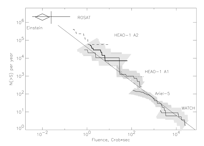
Figure 2: Observed log N-log S distribution for FXTs, assuming a power law fluence distribution ($N(>S)=A_{0}\times S^{-\alpha}$). The thick solid line is best-fit power law derived from a maximum likelihood fit to Ariel-5, HEAO-1, and WATCH data, with $\alpha=0.95$ and $A_{0}=4\times 10^{4}$ The shadowed areas show the measurements of the log N-log S distribution from each experiment, including both event statistics and systematic errors. The cross denotes ROSAT events V (98), and the diamond Einstein FXTs The dashed and dotted curves show the range of distribution that follow from the HEO-1 A2 events, given extreme possibilities for event duration. GHH (96)

Our distribution ( $\alpha=0.95$ and $A_{0}=4\times 10^{4}$, 70% Crab-like vs. 30% thermal spectra) is shown on Fig.2. It is not significantly different from the distribution that follows if we assume that all bursts have a Crab-like spectra.

Fig.2 also shows the segments of the distribution seen by the individual instruments (our analysis approach #2). The shaded areas represent 1$\sigma$ errors for the individual experiment log N-log S curves, including the normalization and the statistics of the number of events seen by each experiment.

Although the duration of the HEAO-1 events is quite uncertain, this uncertainty does not affect the overall distribution. We plot the backward-derived log N-log S assuming the geometric-mean time duration discussed above. But because the overall distribution has a slope close to 1, changes in the assumed duration simply slide the log N-log S contribution from the HEAO-1 instruments up or down along the same curve. The dashed/dotted boundaries show the effect of changing the duration to the extreme possibilities on the HEAO-1 A2 log N-log S distribution.

The ROSAT results from V, 98 and Einstein results from GHH, 96 were not used to determine our net log N-log S distribution. However, they are plotted on Fig.2 for comparison. We have translated the fluence measured in the ROSAT energy band to 2-10 keV by assuming a Crab-like spectrum with negligible foreground absorption. The events reported by V, 98 had fluences from 3.5 to 200 mCrab$\times$sec. We estimated the total number of events per year for ROSAT events which had no detectable quiescent emission as $\sim$2$\times$10⁶ year^-1, and for events without optical counterparts as $\sim$4$\times$10⁵ events year^-1. We have taken these values as upper and lower limits to the FXT rate at this fluence (shown as the cross on Fig.2) The Einstein data were also converted to 2-10 keV assuming a Crab-like spectrum (shown as the rhomb on Fig.2), which is consistent with the spectral shape found by GHH, 96 for hard events.

Our integrated distribution is consistent with a power-law with a slope $\alpha=-1.0^{+0.2}_{-0.3}$. A spatially homogenous distribution of identical sources (standard candles) would have a slope -1.5. Our distribution is consistent with the slope of $\simeq$0.8 derived by PM83 from Ariel-5 events. By adding data from several other experiments, we have extended the PM83 distribution by several orders of magnitude towards the faint end. The ROSAT and Einstein points, derived from V, 98 and GHH, 96, are consistent with an extrapolation of our log N-log S curve.

Fig.3 shows the sky distribution of the events used in Fig.2 (Ariel, HEAO, and WATCH marked with crosses, and ROSAT and Einstein events marked with triangles). The sky distribution is consistent with isotropy. The dipole moment of the distribution towards Galactic Center is 0.07$\pm$0.08 , and the quadrupole moment is 0.31$\pm$0.04 (for an isotropic distribution the dipole moment is zero, and the quadrupole moment is 1/3). We see no significant anisotropy for any subset of these data. However we need to note that there are no reliable exposure maps for mentioned above experiments, making it difficult to be definite about the lack of a disk population in these data.

4 The Connection to GRB

The connection between FXTs and GRBs is especially intriguing. As a result of the Ginga and WATCH studies of prompt X-ray emission from GRBs Strohmayer et al. (1998); Sazonov et al. (1998), and the BeppoSAX discovery of GRB afterglows Piro et al. (1998), it is evident that GRBs can emit a large fraction of their energy in the X-ray region (see also Frontera et al. 2000a, ). This emission is both coincident in time with the gamma-ray burst (prompt emission) and delayed (afterglow). Recently BeppoSAX has found a few GRB-like events with very little or no gamma-ray emission but strong X-ray emission Heise & in’t Zand (2001); Heise et al. (2001). These events were designated “X-ray flashes” Heise & in’t Zand (2001). However, Kippen et al. (2001, 2002) argue that they merge smoothly with regular gamma-ray bursts in a single distribution of their parameters. Such X-ray rich GRBs were estimated to total about 30% of all GRBs Kippen et al. (2002). Whether XRFs and GRBs originate from a single class of progenitors with a smooth distribution of parameters, or are at least in some cases intrinsically different, is not yet clear. Comparison of GRBs and XRFs is fraught with selection effects, including the fact that the observed XRFs were selected in a different energy band (X-rays) than gamma-ray bursts.

In the absence of gamma-ray data, one might classify a conventional GRB that was detected in the X-ray band as an XRF. Grindlay (1999) examined Ariel-5 and HEAO-1 data for an excess of gamma-ray quiet FXTs, above those expected from conventional gamma-ray bursts, that might indicate beaming of GRBs. He estimated that the GRB share of Ariel-5 and HEAO-1 FXT events was about 50%. We wish to refine this estimate by bringing several parameters into our analysis. These include the fraction of GRBs that emit in the X-rays, the ratio of the fluence emitted in the X-ray band to the fluence emitted in the gamma-ray band, the fraction of GRB that produce X-ray afterglows, and the ratio of the X-ray fluence emitted in prompt phase to the fluence emitted in the early afterglow (the first $10^{3}-10^{4}$ sec)

BeppoSAX and WATCH Frontera et al. 2000a ; Sazonov et al. (1998) indicate that the first parameter is close to unity for long-duration GRBs. Long-duration GRBs are defined as events with $T_{90}>2$ sec in the BATSE data set Kouveliotou et al. (1993). The second parameter of interest is the ratio of the fluence emitted in the X-ray band (2-10 keV) to the fluence emitted in the gamma-ray band (50-300 keV), $R_{X/\gamma}$. The ratio $R_{X/\gamma}$ can be estimated from the few events observed in both the X-ray and gamma-ray band, or, using the larger BATSE sample, by extrapolating the measured spectrum into the X-ray band. If the latter is consistent with the former estimate, one could use the full BATSE GRB database to find the $R_{X/\gamma}$ distribution

Band et al. (1993) has shown that GRB spectra can be fit by the expression:

$$N(E)=A\Big{(}\frac{E}{100keV}\Big{)}^{\alpha}exp\Big{(}-\frac{E}{E_{0}}\Big{)},\;\;(\alpha-\beta)E_{0}\geq E,$$

$$N(E)=A\Big{[}\frac{(\alpha-\beta)E_{0}}{100keV}\Big{]}^{\alpha-\beta}\Big{(}\frac{E}{100keV}\Big{)}^{\beta}exp(\beta-\alpha),\;\;(\alpha-\beta)E_{0}\leq E,\;\;(1)$$

in the 20 keV-2 MeV energy band. Using typical values for the parameters (see for example Lloyd & Petrosian, 1999; P, 2000), the average value of $R_{X/\gamma}$ is about several percent. However, Preece et al. (1996) has shown that such an approach leads to an underestimate of X-ray fluxes for about 15% of BATSE GRBs. The magnitude of this underestimate can be relatively high (up to order of magnitude above Band’s formula) for an individual GRB.

Ginga, which was able to simultaneously measure X- and gamma-ray emission from GRBs, found an average ratio of prompt emission $R_{X/\gamma}$ of 0.24 for 22 GRB events, although the logarithmic mean $R_{X/\gamma}$ was 0.07 Strohmayer et al. (1998). $R_{X/\gamma}$ was close to unity for several events. BeppoSAX confirmed that such a high ratio is not rare Frontera et al. 2000a ; Kippen et al. (2002).

Data from different instruments are subject to significant differences in their energy bands and event selection criteria and often do not agree between themselves. To refine our estimate of $R_{X/\gamma}$ we have used all relevant available data including BATSE, Ginga, RXTE, BeppoSAX and WATCH. Fits to the spectra of 53 BATSE and 22 Ginga GRBs, using the Band formula, are found in Band et. al (1993) and Strohmayer et al. (1998). Using the catalog of BATSE GRBs by P, 2000, we have calculated the Band parameters for 81 additional GRBs from BATSE data. For all these bursts we calculated $R_{X/\gamma}$ by integrating the Band formula. Smith et al. (2001) presented RXTE ASM and Konus measurements of 14 GRB in 1.5-12 keV and 50-200 keV energy bands. To convert ASM counts to X-ray fluence we fit the three-color ASM data to a power law for each GRB (assuming a single power law in the 1.5-12 keV region). To obtain the 50-300 keV fluence from the single-channel Konus data we assumed an average value for the Band parameters from P, 2000. BeppoSAX data for 15 GRBs are presented at Frontera et al. (2000a,2000b,2001), in’t Zand et al. (1999,2000a,2000b,2001), Pian et al. (2001) and Nicastro et al. (2001), who give X-ray and gamma-ray fluences for the 2-10 keV and 40-700 keV bands. When available, we used the individual Band’s parameters for each GRB, and otherwise used average values from P, 2000 for 50-300 keV channel.

Sazonov et al. (1998) published a catalog of 95 GRBs detected with WATCH. We used 82 of these events, those for which fluences are available for both energy channels (8-20 keV and 20-60 keV). Full data were unavailable for the other 13 events. For the WATCH data we extrapolated $R_{X}$ and $R_{\gamma}$ to our 2-10 keV and 50-300 keV channels by assuming that the $\alpha$ Band’s parameter was fixed at average value found from Ginga, RXTE and BeppoSAX measurements, $\sim$ -0.85, while the other parameters were fixed at average values from P, 2000.

Fig.4 shows the distribution of $R_{X/\gamma}$ for all these events. The solid line shows the total $R_{X/\gamma}$ distribution derived from the Ginga, RXTE/Konus, BeppoSAX and WATCH measurements (134 GRB total), while the dashed line represents the BATSE events (134 GRB total). Note that the BATSE ratio comes from an extrapolation of the measured spectra to the X-ray band. The non-BATSE events, which are triggered at lower energies than BATSE, tend to have larger median $R_{X/\gamma}$, along with a tail of even higher $R_{X/\gamma}$, X-ray-rich events. We will call them X-ray detected GRB (XDGRB). The later distribution is in a good agreement with BeppoSAX measurements Heise & in’t Zand (2001). We need to note that the $R_{X/\gamma}$ distribution certainly depends on how one weighs events from the different experiments.

We consider the XDGRB estimate of $R_{X/\gamma}$ to be more reliable than the ‘BATSE’ estimate, because the ‘BATSE’ $R_{X/\gamma}$ ratio was calculated by extrapolation of Band’s parameters from the 20 keV-2 MeV region, while for the XDGRB $R_{X/\gamma}$ was actually measured, or calculated using Band’s parameters fit to 2 keV-700 keV measurements. The shift between the peaks of the two distributions is in the direction expected from selection effects (see Appendix).

To determine the integrated X-ray fluence from GRBs, we need to consider not only the prompt emission, but also the afterglow emission (the third and forth parameters mentioned at the beginning of this section). Data from BeppoSAX show that 80-100% of GRBs that emit prompt X-ray emission also show an X-ray afterglow Frontera et al. 2000a . We use this fraction (100 %)as our estimate of the third parameter.

To estimate the fourth parameter (the ratio of the X-ray fluence emitted in the prompt phase to the fluence from the early afterglow) we use predictions of the standard fireball model. The standard fireball model (Wijers, Rees, & Meszaros 1997; Sari, Piran, & Narayan 1998; Sari & Piran, 1999) predicts that in the afterglow phase, the X-ray flux decreases as a power law, as the GRB-induced blast waves sweep up surrounding matter and decelerate. The index of this power law may change its value on time scales from minutes to hours. In this ”external shock” model, both the tail of the prompt X-ray emission and the afterglow are produced by the blast wave (Wijers, Rees, & Meszaros 1997). The external shock model predicts that the amplitude of X-ray prompt emission during the final part of the GRB should be equal to the back-extrapolated flux from the afterglow. This back-extrapolation holds for most GRBs that were observed by BeppoSAX Frontera et al. 2000a .

However, because the afterglow measurements by BeppoSAX start 6-8 hours after the GRB, there is no direct measurement of the X-ray flux immediately after the GRB. If the X-ray afterglow decays as a power law, its integral fluence can reach 50%-200% of the prompt emission Frontera et al. 2000a . We have assembled from the literature decay indices for 15 GRB, and have calculated indices for 10 more, based on the published estimates of prompt and afterglow fluxes. The decay indices $\alpha$ fall in the range -1.0 to -1.9, most commonly about $\sim$1.3, and the distribution of indices can be satisfactorily fit with a Gaussian.

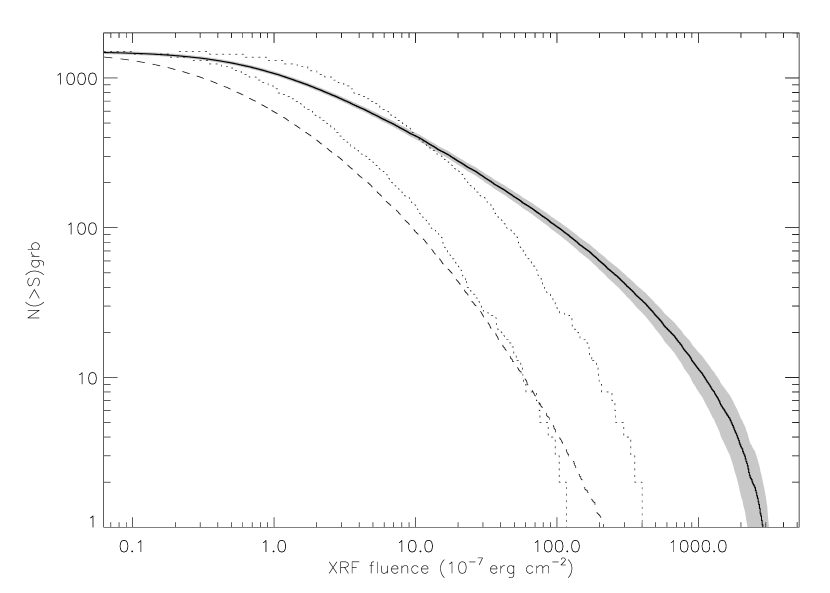
Figure 5: The expected log N-log S X-ray distribution (summing prompt and afterglow emission) for BATSE triggered GRBs, based on different distributions of the $R_{X/\gamma}$ ratio. The thick solid curve is based on the XDGRB distribution $R_{X/\gamma}$, derived from Ginga, BeppoSAX, RXTE/Konus and WATCH events (solid line in Fig.4). The shadowed area shows $1\sigma$ errors for this solid curve, based on Monte Carlo sampling of the $R_{X/\gamma}$ distribution. The dashed curve is based on a $R_{X/\gamma}$ derived from BATSE spectra (‘BATSE’ case). The error region for the ‘BATSE’ case has a similar size as for the XDGRB case. Finally, the dotted curves shows the expected log N-log S distribution for the fixed values of 0.07 and 0.24 found by Ginga (their logarithmic and arithmetic averages; Strohmayer et al., 1998).

In Fig.5, we combine all four parameters discussed above to obtain a log N-log S distribution for X-ray emission from GRBs. This estimate is based on the gamma-ray (50-300 keV) log N-log S distribution for all BATSE GRBs with duration $T_{90}>2$ s. The solid curve is based on our XDGRB distribution of $R_{X/\gamma}$ , sampled by Monte Carlo methods. To the prompt X-ray fluences we add a contribution from the afterglow obtained by Monte Carlo sampling of the afterglow decay parameter $\alpha$ and integrating the afterglow out to $10^{4}$ seconds. These curves plot our estimate of the X-ray fluence from cataloged, triggered BATSE events.

We also show for comparison the expected FXT distributions for less-preferred distributions of $R_{X/\gamma}$: the mean and logarithmic mean of Ginga (0.07 and 0.24, Strohmayer et al., 1998) and our ’BATSE” distribution. The less-preferred $R_{X/\gamma}$ yield numbers of FXTs from GRBs that fall below the preferred estimate.

We would like to understand how these curves would change if we included all the GRBs that are too faint to trigger BATSE. Some of them may be, in fact, X-ray rich GRB or XRFs (see Kippen et al., 2002). We can get some notion of this correction by adding to our sample the sample of untriggered BATSE events obtained by Kommers et al. (1998) and Stern et al. (2000), which enhance the BATSE sample of the faint end. We find little change for all but the faintest part of the XRF log N-log S curve. Fig.6 shows the XRF log N-log S distribution for triggered, untriggered, and all known BATSE GRBs, based on the XDGRB estimate of $R_{X/\gamma}$.

Fig.7 compares our prediction of the FXT’s from GRBs to our best-fit distribution of all FXT. The plotted distribution (solid curve) is based on the XDGRB estimate of $R_{X/\gamma}$, and the population of all (triggered plus untriggered) BATSE GRBs.

The distribution derived from the ‘BATSE’$R_{X/\gamma}$ (shown with dotted curve). BeppoSAX data (Heise, in’t Zand, & Kuulkers 2000, Heise et al., 2001) suggest that about 70% of FXT detected by BeppoSAX are GRB-related. The ‘BATSE’ $R_{X/\gamma}$ would yeld a value of 0.1-1% for this ratio, far less than observed.

Fig.7 also compares our estimate of the log N-log S curve for FXT from GRBs with the rate of candidate GRB afterglows reported by Greiner et al. (2000). For any reasonable assumption about the $R_{X/\gamma}$ distribution, the Greiner et al. (2000) rate of events without optical counterparts is in good agreement with our prediction, suggesting that a substantial fraction of their residual, non-stellar, events are indeed GRBs.

It is clear that the fraction of fast X-ray transients that can be attributed to classical gamma-ray bursts drops with decreasing fluence. The predicted X-ray event rate for “normal” GRBs falls a factor of $\sim$ 3-5 below the total FXT rate at high fluences, but a factor of 100 below at the faint end. Even if we are off by a factor of two or three due to unknown effects, a large majority of FXTs are not counterparts of classical GRBs (e.g, not X-ray flashes), especially at the faint end. However, we cannot rule out a possibility that exists a population of X-ray rich GRB-like events that comprise a large fraction of the FXTs at the faint end.

5 OTHER SOURCES of FXTs

5.1 Possible candidates

The timescales and spectra of FXTs are diverse. Timescales range from seconds to hours, and spectra range from very hard (kT$>$20 keV, Rappaport et al., 1976) to soft (kT$\sim$1 keV, Swank et al., 1978). PM, 83 suggested the time profiles could be divided into classes, perhaps indicating multiple progenitor classes. The few FXT identifications made to date confirm the heterogeneous nature of FXTs.

The lower right corner of our X-ray log N-log S curve is formed by several events with duration up to one day, which were seen mostly by WATCH CT (99). A T Tauri star was suggested by CT, 99 as the progenitor for one of the events, while the rest were probably generated by X-ray binaries. Several X-ray binaries have been recently found to generate short, powerful outbursts that might be classified as FXTs. For example, outbursts from V4641 Sgr up to 12.2 Crab (2-12 keV) with durations less than a day were observed by the RXTE and BeppoSAX (Smith, Levine, & Morgan 1999, in’t Zand et al. 2000b ; Wijnands & van der Klis (2000)).. During the RXTE PCA observation, V4641 Sgr showed X-ray fluctuations by a factor of 4 on timescales of seconds and $\backsim 500$ on timescales of minutes Wijnands & van der Klis (2000). The mass function identifies the system as a high-mass X-ray binary harboring a black hole Orosz et al. (2000). A slightly longer type of X-ray transient, CI Cam, with a single short outburst about 2 days long, was also discovered by RXTE (Smith et al., 1998, Revnivtsev, Emel’yanov & Borozdin 1999).

“Super type I X-ray bursts” that last from 30 min to 3 hours were reported recently from several low-mass X-ray binaries (e.g., Cornelisse et al., 2000; Wijnands, 2001). Similar events might been detected as high-fluence FXTs by low-resolution experiments. These or similar sources might contribute to the lower right corner of the FXT log N-log S curve.

In’t Zand et al. (1998), and Kaptein et al. (2000) announced the discovery of type I X-ray bursts from ‘empty’ places. These bursts, observed from locations without steady emission, would be naturally classified as FXTs. The origin of such bursts might be low accretion rate neutron star binaries. We can get an idea of the rate of ‘empty’ place bursts from BeppoSAXin’t Zand (2001). It observed the Galactic Center region for $T_{obs}=4\times 10^{6}$ s and detected about $\sim$1500 X-ray type I bursts from $N_{b}$=31 sources. At the same time it observed $B_{e}$=4 X-ray type I bursts from 4 ‘empty place’ X-ray bursters. If all these events were generated on low-accretion X-ray neutron stars (with, say, X-ray luminosity less than several percent of the Eddington limit), and their space distribution follows the space distribution of normal X-ray bursters, we can estimate the total number of bursts from ‘empty place’ per year per sky as: $N_{sky}=(1_{year}/T_{obs})\cdot(N_{t}/N_{b})\cdot B_{e}\sim 50$ events, where $N_{t}\sim$ 50 is the total number of known normal bursters. If their distribution is isotropic, the number of bursts from ‘empty’ places would be at least an order of magnitude greater.This simplified estimate agrees well with the BeppoSAX estimate Cornelisse et al. 2002a . They found that the total number of such sources in our Galaxy is between 30 and 4000, while the recurrence time between the bursts is a half year (for 30 sources) and several tens of years (for 4000 sources) The fluence from such events would be comparable with outbursts from RS CVn binaries, yielding about 50-100 events per sky in the $10-1000Crab\times sec$ region.

PM, 83 identified a large fraction (6 out of 27) of Ariel-5’s fast X-ray transients with RS CVn binary systems. Another RS CVn object was proposed as a possible FXT source by AW, 86. RS CVn systems are binaries formed by a cool giant or subgiant with an active corona and a less massive companion in a close synchronous orbit. RS CVn binaries typically exhibit a peak flux $\sim$10³² erg/s for a duration of 1 to 10 h. Outbursts from nearby RS CVn systems would have a fluence that puts them in the middle part of our diagram. This is certainly true for the identifications proposed by PM, 83 and AW, 86.

Our analysis of GRB X-rays indicates that this contribution to the FXT log N-log S is most significant around 100-1000 Crab$\times sec$. Heise et al. (2000) reported that about 70% of all FXTs detected with BeppoSAX are GRB-related, i.e., either conventional GRBs or XRFs. 1 Our best estimate (XDGRB) indicates that the GRB contribution to FXTs (see $R_{X/\gamma}$ distribution discussion) peaks at 20-30%. However, taking into account the uncertainties of both studies, we consider these results as moderately consistent between themselves, and consistent with Grindlay, 1999. We note that BeppoSAX/WFC detected $\sim$1.5$\times$10³ thermonuclear X-ray bursts from $\sim$35 sources, but did not classify them as FXTs because they had clear identifications. Some of these bursts might have been identified as FXTs by earlier experiments like Ariel-5. This would increase the total number of FXTs and decrease the GRB fraction. Our estimate of GRB-related FXTs is also consistent with the ROSAT result Greiner et al. (2000) at low fluences. We have shown (see Fig.7) that the contribution of classical BATSE GRBs drops dramatically for lower fluences. Other sources must dominate FXT statistics that region.

C, 86 found 6 of their 10 FXTs to be flares from late type dMe-dKe stars, i.e., M or K dwarfs with Balmer lines in emission. AW, 86 also identified 3 of 10 HEAO-1 A1 FXTs with flare stars. Flares of dKe-dMe have peak fluxes of 10²⁸-10³² erg s^-1 and duration from $\sim$minutes to $\sim$hours. Their spectra have temperature $\sim$1 keV, and they should be well detected by ROSAT. Indeed, V, 98 found star-like counterparts for 132 out of 141 reported FXTs. We therefore suggest that the least luminous and most numerous part of log N-log S distribution is formed by nearby flare stars.

There is however a fraction of lower-fluence FXTs that are not identified with star-like objects. While the contribution of classical GRBs should be negligible in this region, other types of progenitors may play a more important role. One of them, gamma-ray quiet GRBs might arise in several ways (e.g. MacFayden & Woosley, 1999; Meszaros & Gruzinov, 2000). Recent BeppoSAX results have shown that some GRBs are faint in the standard 50-300 keV BATSE band but bright in X-rays Kippen et al. (2001, 2002). Out of the 53 GRB-like transients detected with the BeppoSAX WFC, 17 were not registered by BeppoSAX GRB monitor, which is sensitive in 40-400 keV energy region. Kippen et al., 2001 found that 9 of such XRFs were also seen by BATSE and recorded as untriggered events at BATSE database. According to Sazonov et al. (1998) 10% of WATCH events had detectable emission in 8-20 keV energy channel but no significant emission in the hard channel. Our analysis (see Fig.6) confirms that untriggered BATSE events contribute only modestly to the lower fluence part of log N-log S if they follow the same $R_{X/\gamma}$ distribution as the triggered events. But GRB-like outbursts with softer spectra might be more significant at lower fluences.

Other exotic progenitors may contribute also. Schafer, King, & Deliyannis 2000, suggested that ordinary main sequence stars like our Sun may exhibit rare powerful superflares with $10^{33}$ - $10^{38}$ ergs, some of them in X-rays. However, one cannot quantify their contribution until one better understand the frequency of such superflares.

Extragalactic sources may also generate FXT phenomena. X-ray variability is a fundamental property of Active Galactic Nuclei. In the last decade it was found that BL Lac objects (blazars) exhibit strong correlated variability in both X-ray and TeV gamma-ray bands on short timescales of days to hours Catanese et al. (1997); Marachi et al. (1999). The brightest of such events may be detected as FXTs.

5.2 Contributions to the Fluence Distribution

Previous searches for FXT progenitors demonstrated that we probably deal with a mix of close (flare stars) and extragalactic (GRB-related) events. The sky distribution for both these populations is expected to be isotropic. This is consistent with the sky distribution of detected FXT (Fig.3). However, the absense of reliable exposure maps for many observations and possible selection effects leave room for the existence among FXTs of a non-isotropic population with the Galactic disk or bulge distribution. The slope of the log N-log S distribution of such additional component is expected to be flatter than -1.5 for a variety of possible progenitors.

The most natural candidates for an additional component of FXTs are low mass X-ray binaries (LMXBs). Cornelisse et al. 2002b, have analyzed BeppoSAX data and found several X-ray type-I bursts from ’empty’ places, where no persistent emission was detected down to a several mCrab limit. Cocchi et al., 2001 have proposed a new class of low-luminosity bursters. Cornelisse et al. 2002b, have shown that all detected bursts from ’empty’ places are indeed the members of such class and follow LMXB space distribution. Since LMXBs are concentrated in the Galactic Bulge (see e.g. recent review by Grimm, Gilfanov, & Sunyaev 2002), any associated extra FXTs should be clustered around the Galactic Center. However, most early surveys had difficulty in detecting FXTs from this part of the sky Warwick et al. (1981). Their localization accuracy was poor (typically several degrees), and any X-ray flash from a populated region of the sky would tend to be attributed to known X-ray sources. Hence, the population of LMXB with low persistent flux and emitting rare bursts would need to be be quite numerous to have been clearly detected by those instruments. Emel’yanov et al. (2001) have shown that TTM observations of the Galactic Bulge put strong constraints on the number-frequency function of low-accreting X-ray bursters indicating that the number of low-luminosity X-ray bursters $\times$ the burst frequency from a burster is small. If the FXTs that are distributed as a bulge population are fewer than several percent of all FXTs, they cannot be found with the usual statistical tests (e.g., a K-S test would not identify a bulge fraction less than 3% of the total as significant). The deviation from uniformity in the FXT distribution would be further masked by the poor ability of previous studies to find FXTs at low latitudes (see e.g. Warwick et al., 1981, for the discussion of source confusion in Ariel-5 survey).

Our two most reliably identified source populations, gamma-ray bursts and stellar flares, although isotropically distributed, might yield a log N-log S distribution with a slope significantly flatter than -3/2 (as would be expected for a uniform distribution of standard candles). In the case of gamma-ray bursts, the distribution is known to flatten due to cosmological effects. Even more important than the cosmological flattening, the luminosity distribution of FXTs from GRBs is flattened by the broad distribution of $R_{X}/R_{\gamma}$. We demonstrate below that nearby flare stars would also produce a distribution flatter than -3/2.

EXOSAT observed 22 late-type flare stars (dMe-dKe) in the vicinity of the Sun (2-20 pc) in the 1-10 keV energy region. They found that these stars generated X-ray flares with total energies from 10³⁰ to 10³⁴ ergs and $N(>E)\sim E^{-0.7}$ (Pallavicini, Tagliaferri, & Stella 1990), e.g. with a differential frequency-flare distribution fits a power law N(E)$\sim E^{-1.7}$. A similar distribution function has been observed for the Sun, with differential frequency-flare energy distribution index $\Gamma=1.8$ Gershberg (1989) or 2.0 Veronig et al. (2002), and for optical flares on the M dwarf flare star AD Leo (Pettersen, Coleman & Evans 1984).

The integral distribution of X-ray flares from flare stars is:

$$N(>S)\propto\int\limits_{r=R_{min}}^{\infty}\int\limits_{E=4\pi r^{2}S}^{\infty}n(r,E)dEdr,\;\;(2)$$

where $n(r,E)\propto r^{2}\times E^{-\gamma}$ is the differential distribution function of X-ray flares from flare stars, E is the flare energy, $R_{min}$ is the nearest flare star, and S=E/(4 $\pi r^{2}$) is the measured fluence. This distribution holds for sources uniformly distributed through the space (as is certainly within a radius of 100 pc), with a differential frequency- flare energy function described with power law $E\propto E^{-\gamma}$. We derive:

$$\int\limits_{E=4\pi r^{2}S}^{\infty}E^{-\gamma}dE=(4\pi r^{2}S)^{-\gamma+1}\propto r^{2-2\gamma}\times S^{1-\gamma}\;\;(3)$$

substituting $\gamma=\alpha+1$, where $\alpha$ is the slope of the cumulative frequency-flare energy function, we get:

$$N(>S)\propto S^{-\alpha}\times\int\limits_{r=R_{min}}^{\infty}r^{2-2\alpha}dr\;\;(4)$$

If the total flare energy dynamical range $E=E^{-\gamma}[E_{min},E_{max}]$, is greater than the distance dynamical range $R^{2}[R=(R_{min},R_{max})]$, then for a range of detected fluences $S=[E_{min}/R_{min}^{2},E_{max}/R_{max}^{2}]$ the slope of the detected cumulative number-fluence function $(N(>S))$ will be the same as the slope of the integral frequency- flare energy function $N(>E)\propto E^{-\alpha}$

EXOSAT data confirm that $N(>E)\propto E^{-0.7}$ for at least $E_{max}/E_{min}=10^{4}$ (Pallavicini, Tagliaferri, & Stella 1990). So, for example, if $R_{1}^{2}/R_{2}^{2}=100$, the dynamical range where $N(>S)\propto S^{-0.7}$ is $S_{1}/S_{2}=100$.

Integrating over the full range of distances (2-100 pc) and flare energies ($10^{31}$-$10^{34}$), we estimate that the integral fluence distribution $(N(>S))$ from stellar flares has a slope that steepens slowly from $-\alpha$ to -3/2 with increasing fluence (Fig.8). Note that over 3 orders of magnitude in fluence, it is close to a power-law with slope $\sim-0.6\approx-\alpha$.

The intrinsic distribution of flare energy drives the observed log N-log S fluence distribution for the stellar component of FXTs. The fluence (Crab$\times$s) in the 2-10 keV region is related to the flare energy as $3\times 10^{30}$ (erg) $\times$ M (at Crab$\times$sec) $\times$ $D^{2}$ (at $pc^{2}$). The HEAO-1 experiments had a fluence detection threshold about 1 Crab$\times$s, while Ariel-5 had a threshold of about 100 Crab$\times$s. As a result, HEAO-1 detected flares with energy $L\geq 1\times 10^{31}$ ergs from sources located within 2 pc, and the most energetic flares from distances up to 100 pc. Ariel-5 was able to detect flares with $L\geq 1\times 10^{33}$ within 2 pc, and assuming the most energetic flares within 10 pc. Taking the star density near the Sun $\sim$0.1 star $pc^{-3}$, and assuming, based on the standard 4-component model of the Galaxy Bahcall & Soneira (1986),that stars are distributed uniformly within 100 pc of the Sun, HEAO-1 should have seen flares from up to $4\cdot 10^{5}\times K_{fs}$ flare stars, while Ariel-5 was able to detect $400\times K_{fs}$ flare stars. The catalog of chromospherically active stars Strassmeier et al. (1993) includes 3 stars closer than 10 pc, while Pallavicini, Tagliaferri & Stella (1990) observed 12 flare stars within 10 pc. Basing on these data we accept $K_{fs}=2.5\cdot 10^{-3}$ as a lower limit for fraction of dMe-dKe stars around the Sun. In this case the HEAO-1 experiments were able to detect X-ray flares from $10^{4}$ flare stars. Because the HEAO-1 experiments were sensitive to fainter events than Ariel-5, and because flare star FXTs are generally fainter than RS CVn FXTs, we expect that the ratio between late-type flare stars and RS CVns should increase as we move from the Ariel-5 to the HEAO-1 fluence band. This is consistent with their proposed identifications: HEAO-1 identified 10 events with dMe-dKe stars, while Ariel-5 reported only one such identification.

In summary, over a wide range of fluences, the intrinsic distribution of flare energies dominates over the geometric term, so that the -3/2 power law expected for standard candles does not apply. The shallow slope of the FXT distribution is, therefore, obtained naturally even for uniformly distributed progenitors.

6 SUMMARY

We have produced a composite log N-log S relationship for fast X-ray transients, by combining data from several experiments. This relation spans 4 orders of magnitude, and is fit to a power law with a slope of $-1.0^{+0.2}_{-0.3}$. Extrapolation of this slope to lower fluences is consistent with the sensitive ROSAT and Einstein experiments. The sources of fast X-ray transients are undoubtedly heterogeneous. The $\alpha\sim$ -1 power law must come from the summation of contributions from several different progenitor classes. Both GRBs and flares stars will contribute components to this distribution that are flatter than the ‘isotropic’ slope of $\alpha=-3/2$. The exact shape of the global fluence-frequency relationship might deviate from this simple power law, even inside the range we measured. However, due to the small number of events that we analyzed, and resulting large uncertainty in the deduced rate, a more complicated luminosity function is not justified (see for example detailed discussion at Murdoch, Crawford, & Jauncey (1973)).

We use archival measurements of the X-ray and gamma-ray fluences for 134 GRB to estimate the distribution of the X-ray to gamma-ray ratio. This $R_{X/\gamma}$ distribution shows the presence of highly significant tail of X-ray rich events. Extrapolating from the BATSE GRB catalog, we find that the fraction of fast x-ray transients attributable to classical gamma-ray bursts is a function of fluence, being greatest for high fluences and dropping dramatically at the faint end. The exact fraction of GRB-associated fast X-ray transients is sensitive to our assumptions about the $R_{X/\gamma}$ distribution, but our analysis certainly shows that most of fainter FXTs are not counterparts of classical gamma-ray bursts. The fraction of FXTs from non-GRB sources, such as magnetic flares on nearby stars, is the highest for the faintest flashes.

Our understanding of the fast X-ray transient phenomenon is still poor. The situation is similar to that for gamma-ray bursts before BATSE. There have been many FXTs detected, but by a variety of instruments each with specific restrictions. The data show convincingly that FXTs are ubiquitous. But the number of events detected by each particular experiment is small, and their statistical analysis is complicated. We can identify some classes of progenitor sources, but we can determine the fractional contribution of these classes only roughly. There remains room for the discovery of new types of sources that produce fast X-ray transients, but we certainly cannot yet confirm the existence of new classes like “gamma-ray quiet GRBs” or “superflares” at normal stars. A large uniform dataset from a dedicated, sensitive wide-field X-ray experiment (see e.g. Fraser et al., 2002; Priedhorsky et al., 2000; Borozdin et al., 1999) could revolutionize our understanding of the FXT phenomenon. The greatest opportunity for discovery may lie in the faintest FXTs, posing a challenge to instrument builders.

Appendix A Appendix. Selection effects on $R_{X/\gamma}$ ratio

Differences in the sensitivity band and observational strategy significantly affect the $R_{X/\gamma}$ ratio measured with different instruments. In our analysis we made use of all data we aware of to obtain the most instrument-independent estimate possible. We calculated the mean, median and variance of the measured distributions of $R_{X/\gamma}$ for the ‘BATSE’ and XDGRB samples (Table 1) We also fitted the distribution $R_{X/\gamma}$ for the XDGRB and ‘BATSE’ samples with a Gaussian, and with a Gaussian plus quadratic polynomial. These functions were choosen simply to match the data with a smooth curve. A Gaussian alone cannot fit the tail of distribution. The difference between the Gaussian cores of the distribution is in the direction expected from the triggering effects, but the tail in the XDGRB distribution cannot be caused by triggering effects. The inset on Fig.4 shows the best-fit curves for the Gaussian plus quadratic polynomial fit to the both samples, to show qualitatively how they differ.

To understand the effect of triggering on the $R_{X/\gamma}$ distribution, we consider the simplified case in which the X-ray/gamma-ray fluence ratio follows a log-normal distribution. In other words, if $\alpha$ is defined as $F_{x}\tbond exp(\alpha)F_{\gamma}$, $\alpha$ is distributed as a Gaussian. The Gaussian distribution of $\alpha$ is dN/d$\alpha\propto exp[-(\alpha-\mu)^{2}/2\sigma^{2}]$, where $\mu$ is the mean of the distribution and $\sigma$ is its standard deviation, for events triggered in the band of $F_{\gamma}$.

If the log N-log S distribution goes as $N\sim S^{-\beta}$, then the X-ray triggered distribution of $\alpha$, for the same population of events, will follow a Gaussian distribution of the same width, but centered on $\mu(X_{ray})=\mu(\gamma)+\beta\cdot\sigma$. We assume that the X-ray trigger band is the same band as for $F_{X}$. In the case of an isotropic, $\beta=3/2$ power law, the distribution will be displaced 1.5 standard deviations to the right when we trigger on X-rays instead of gamma rays. For trigger bands other than those used for $R_{X}$ or $R_{\gamma}$, the displacement will be different.

This selection effect may explain the fact that WATCH generally selects softer GRBs than BATSE. While BATSE triggers in the 50-300 keV band, WATCH triggers in the 8-100 keV band. However, the nominal trigger range for Ginga, at 50-400 keV is harder even than BATSE. The softer $R_{X/\gamma}$ ratio obtained by Ginga may be the result of a secondary selection done by Strohmayer et al. (1998). While Ginga observed about 120 GRBs Ogasaka et al. (1991); Fenimore et al. (1993), only the GRBs with good quality spectral data in both $\gamma$- and X-ray detectors were selected for spectral analysis, possibly driving the selection of softer, X-ray bright, GRBs.

We can make a rough check of the selection effect by taking the power law $\beta$ from BATSE measurements, calculating the displacement $\beta\cdot\sigma$, and comparing it with the displacement between the BATSE and the other, mostly X-ray triggered, $R_{X/\gamma}$ distributions. We predict a displacement for $\beta\sim$ 1.3 (derived from middle part of BATSE GRBs log N-log S) of 0.6-0.7, compared to a displacement in range of 0.5-0.7 (Table 1), between the $R_{X/\gamma}$ distributions for ‘BATSE’ and XDGRB. The direction is as expected: triggering at softer energies moves the $R_{X/\gamma}$ distribution to larger values.

We have tested whether the difference between the ‘BATSE’ and XDGRB distributions was caused by the effect of trigger-band selection on a single distribution of GRBs, or if there existed an additional X-ray rich GRB population not detected by BATSE. To do this we have fit the $R_{X/\gamma}$ distribution of the BATSE GRB sample to a log-normal distribution. A maximum-likelihood estimate of the fit parameters gives $\mu(X_{ray})\approx 0$ and $\sigma=0.5$. This result shows that except of the triggering band effect there is also an additional contribution of X-ray rich events for XDGRB case .

Figure 1: Maximum-likelihood confidence limits for the parameters of a $N(>S)=A_{0}\times S^{-\alpha}$ power-law distribution of FXTs. The contour lines show 1, 2, and 3 $\sigma$ significance levels.

Figure 3: Sky distribution of the FXTs included in the log N-log S distribution of Fig.2. The crosses are the Ariel-5, HEAO-1, and WATCH events; triangles are the ROSAT and Einstein events

Figure 4: $R_{X/\gamma}$ distribution for GRBs. (2-10 keV fluences /50-300 keV fluences). The solid line is from Ginga, RXTE/Konus, BeppoSAX, and WATCH events (XDGRB case), and the dashed line from BATSE events. The former were measured in the X-rays, but the latter were extrapolated from the BATSE band (above 20 keV) to the X-rays. The inset shows the best fit to these distributions, using a Gaussian plus a quadratic polynomial (fit parameters are given at Table 1). The solid curve is the XDGRB sample, and the dashed curve is the ‘BATSE’ sample.

Figure 6: The dashed curve is the expected XRF log N-log S for triggered BATSE GRB, with $T_{90}>2$ sec, using the XDGRB estimate of $R_{X/\gamma}$ (as for the solid line of Fig.4). The dotted curve is the expected contribution from untriggered BATSE GRB, assuming the same $R_{X/\gamma}$ distribution, and the solid curve is sum of the triggered and untriggered contributions. The small difference suggests that undetected GRBs are unlikely to make a significant contribution to the FXT distribution.

Figure 7: Contribution of gamma-ray bursts to the model log N-log S distribution for X-ray flashes. The XRF distribution parameters are taken from Fig.1. The thin solid curve is the GRB-derived distribution from Fig.6 (XDGRB case), while the thin dotted curve is the expected distribution from the ‘BATSE’ case. The cross is derived from the ROSAT survey of afterglow-like events that were not attributed to late-type stars Greiner et al. (2000). Despite the uncertainties in our analysis, it is clear the classical gamma-ray bursts are more important contributor to bright XRFs than to faint XRFs.

Figure 8: The expected log N-log S FXT distribution for late-type flare stars in the vicinity of the Sun. The normalization is arbitrary. The slope for lower fluences is dominated by the intrinsic number-energy distribution of stellar flares, rather than the 3/2 slope of standard candles in an isotropic geometry.

Table 1: log($R_{X/\gamma}$) distribution parameters for different models

Case	Distribution			Model parameters
	parameters			Gaussian		Gaussian + Quadratic polynomial
	Mean	Median	$\sigma$	$\mu$	$\sigma$	$\mu$	$\sigma$	Ac	Bc	Cc
BATSEa	-1.67	-1.68	0.48	-1.53	0.43	-1.53	0.43	0.0	0.0	0.0
XDGRBb	-0.95	-1.12	0.68	-1.06	0.30	-1.08	0.22	-0.01	-0.01	0.04

• ^a BATSE events

• ^b Ginga + WATCH + RXTE + BeppoSAX events, XDGRB case

• ^c A, B & C represent parameters of the quadratic polynomial $Ax^{2}+Bx+C$

References

- AW (86) Ambruster, C., & Wood, K. 1986, ApJ, 311, 258 (AW86)
- Bahcall & Soneira (1986) Bahcall,N. & Soneira, R. 1986, ApJ, 311, 15
- Band et al. (1993) Band, D., Matteson, J., Ford, L., et al. 1993, ApJ, 413, 281
- Borozdin et al. (1999) Borozdin, K.N., Priedhorsky, W.C., Arefiev, V.A., et al. 1999, in: Small Missions for Energetic Astrophysics : Ultraviolet to Gamma-Ray : Los Alamos, New Mexico, February 1999, Ed.: S.P. Brumby, AIP Conference Proc., 499, 20
- CT (99) Castro-Tirado, A., Brandt, S., Lund, N., & Sunyaev, R. 1999, A&A, 347, 927 (CT99)
- Catanese et al. (1997) Catanese, M., Bradbury, S., Breslin, A., et al. 1997, ApJ, 487, L143
- Cocchi et al. (2001) Cocchi, M., Bazzano. A., Natalucci. L., Ubertini. P., Heise. J., Kuulkers. E., Cornelisse. R., & in’t Zand J. 2001, A&A, 378, L71
- C (86) Connors, A., Serlemitsos, P., & Swank, J. 1986 ApJ, 303, 769 (C86)
- Cornelisse et al. (2000) Cornelisse, R., Heise, J., Kuulkers, E., Verbunt, F., & in’t Zand J. 2000, A&A, 357L, 21
- (10) Cornelisse, R., Verbunt, F., in’t Zand J., Kuulkers, E., Heise, J., Remillard, R., Cocchi, M., Natalucci, L., Bazzano, A., & Ubertini P. 2002a, A&A, in press (astro-ph/0207135)
- (11) Cornelisse, R., Verbunt, F., in’t Zand J., Kuulkers, E., & Heise, J. 2002b, A&A, in press (astro-ph/0207138)
- Emel’yanov et al. (2001) Emel’yanov, A., Arefiev, V., Churazov, E., Gilfanov, M., Sunyaev, R., & Skinner, J. 2001, AstL, 27, 12, 908
- Fenimore et al. (1993) Fenimore et al. 1993, in AIP Conf. Proc. 280, CGRO, ed Friedlander, M., Gehrels, N., & Macomb, D. (New York: AIP), 917
- Fraser et al. (2002) Fraser, G.W., Brunton, A.N., Bannister, N.P. et al. 2002, Proc. SPIE, 4497, 115, in: X-Ray and Gamma-Ray Instrumentation for Astronomy XII, Eds.: K.A. Flanagan, O.H. Siegmund
- (15) Frontera, F., Amati, L., Costa, E., et al., 2000, ApJS, 127, 59
- (16) Frontera, F., Antonelli, L., Amati, L., et al. 2000, ApJ, 540, 697
- Frontera et al. (2001) Frontera, F., Amati, L., Vietri, M., et al. 2001, ApJ, 550, L47
- Gershberg (1989) Gershberg,. R., 1989, Mem. Soc. Astron. Ital. 60, 263
- GHH (96) Gotthelf, E., Hamilton, T., & Helfand, D. 1996, ApJ, 466, 779 (GHH96)
- Greiner et al. (2000) Greiner, J., Hartmann, D., Voges, W., Boller, T., Schwarz, R., & Zharikov, S. 2000, A&A, 353, 998
- Grimm, Gilfanov, & Sunyaev (2002) Grimm, H., Gilfanov. M., Sunyaev. R. 2002, A&A, in press (astro-ph/0109239)
- Grindlay (1999) Grindlay, J. 1999, ApJ, 510, 710
- Heise, in’t Zand, & Kuulkers (2000) Heise, J., in’t Zand, J., & Kuulkers, E. 2000, HEAD, 32.2803
- Heise & in’t Zand (2001) Heise, J., & in’t Zand, J., 2001, in: Gamma-Ray Bursts in the Afterglow Era, Proceedings of the International workshop, Rome, 17-20 October, 2000. Ed: E. Costa, F. Frontera, and J. Hjorth. Berlin Heidelberg: Springer, 2001, p. 16.
- Heise et al. (2001) Heise, J., in’t Zand, J., Kippen M., & Woods P., 2001, preprint (astro-ph/0111246)
- Holt & Priedhorsky (1987) Holt, S., & Priedhorsky, W., 1987, Space Sci.Rev., 45, 269
- Kaptein et al. (2000) Kaptein, R., in ’t Zand, J., Kuulkers, E., Verbunt, F., Heise, J., & Cornelisse R. 2000, A&A358L, 71
- Kippen et al. (2001) Kippen, M., Woods, P., Heise, J., in’t Zand J., Preece, R., & Briggs, M. 2001, in: Gamma-Ray Bursts in the Afterglow Era, Proceedings of the International workshop, Rome, 17-20 October, 2000. Ed: E. Costa, F. Frontera, and J. Hjorth. Berlin Heidelberg: Springer, 2001, p. 22.
- Kippen et al. (2002) Kippen, M., Woods, P., Heise, J., in’t Zand J., Briggs, M., & Preece, R. 2002, preprint (astro-ph/0203114)
- Kommers et al. (1998) Kommers, J., Lewin, W., Kouveliotou, C., van Paradijs, J., Pendleton, G., Meegan, C., & Fishman, G. 1998, A&AS, 193, 7907
- Kouveliotou et al. (1993) Kouveliotou, C., Meegan, C., Fishman, G., Bhat, N., Briggs, M., Koshut, T., Paciesas, W., & Pendleton, G. 1993, ApJ, 413, L101
- Lee & Petrosian (1996) Lee, T., & Petrosian, V. 1996, ApJ, 470, 479
- Lloyd & Petrosian (1999) Lloyd, M., & Petrosian, V. 1999, ApJ, 511, 550
- MacFayden & Woosley (1999) MacFayden, A., & Woosley, S. 1999, ApJ, 524, 262
- Marachi et al. (1999) Maraschi, L., Fossati, G., Chiappeti, L., et al. 1999, ApJ, 526 L81
- Meszaros (2002) Meszaros, P.,2002, Annu.Rev.Astron.Astrophys., 40 (also astro-ph/0111170)
- Meszaros & Gruzinov (2000) Meszaros, P., & Gruzinov, A. 2000, ApJ, 543, L35
- Meszaros, Rees, & Wijers (1998) Meszaros, P., Rees, M., & Wijers, R. 1998, ApJ, 499,301
- Murdoch, Crawford, & Jauncey (1973) Murdoch, H., Crawford, D., & Jauncey, D 1973, ApJ, 183,1
- Nicastro et al. (2001) Nicastro, L., Cusumano, G., Antonelli, A., et al. 2001, preprint (astro-ph/0104131)
- Ogasaka et al. (1991) Ogasaka, Y., Murakami, T., Nishimura, J. Yoshida, A., & Fenimore, E. 1991, ApJ, 383, L61
- Orosz et al. (2000) Orosz, J., Kuulkers, E., van der Klis, M., et al. 2000, AAS, 197.8320
- Pallavicini, Tagliaferri & Stella (1990) Pallavicini, R., Tagliferri, G., & Stella, L. 1990, A&A, 228, 403
- Pettersen, Coleman & Evans (1984) Pettersen, B., Coleman, L., & Evans, D. 1984, ApJS, 54, 375
- Petrosian & Lee (1996) Petrosian, V., & Lee, T. 1996, ApJ, 467, L29
- Pian et al, (2001) Pian, E., Soffitta, P., Alessi, A., et al. 2001, A&A, 372, 456
- Piro et al. (1998) Piro, L., Amati, L., Antonelli, L., et al. 1998, A&A, 331, L41
- Preece et al. (1996) Preece, R., Briggs, M., Pendleton, G., Paciesas, W., Matteson, J., Band, D., Skelton, R., & Meegan, C. 1996, ApJ, 473, 310
- P (2000) Preece, R., Briggs, M., Mallozzi, R., Pendleton, G., Paciesas, W., & Band, D. 2000, ApJS, 126, 19 (P2000)
- Priedhorsky et al. (2000) Priedhorsky, W.C., Fraser, G.W., Borozdin, K.N., Arefiev, V. A., AAS HEAD meeting, 32, 39.13
- PM (83) Pye, J., & McHardy, I. 1983, MNRAS, 205, 875 (PM83)
- Rappaport et al. (1976) Rappaport, S., Buff, J., Clark, G., Lewin, W., Matilsky, T., McClintock, J. 1976, ApJ, 206, L139
- Revnivtsev, Emel’yanov, & Borozdin (1999) Revnivtsev, M., Emel’yanov, A., & Borozdin, K. 1999, AstL, 25, 294
- Sari, Piran, & Narayan (1998) Sari, R., Piran, T., & Narayan, R. 1998, ApJ, 497, L17
- Sari & Piran (1999) Sari, R., & Piran, T. 1999, A&AS, 138, 537
- Sazonov et al. (1998) Sazonov, S., Sunyaev, R., Terekhov, O., Lund, N., Brandt, S. & Castro-Tirado, A. 1998, A&AS, 129, 1
- Schafer, King, & Deliyannis (2000) Schafer, B., King, J., & Deliyannis, C. 2000, ApJ, 529, 1026
- Smith et al. (1998) Smith, D., Remillard, R., Swank, J., Takeshima, T., & Smith, E. 1998, IAU Circular, 6855
- Smith, Levine, & Morgan (1999) Smith, D., Levine, A., & Morgan, E. 1999, IAU Circular, 7253
- Smith et al. (2002) Smith, D., Levine, A., Bradt, H., et al. 2002, ApJS, 141, 415
- Stern et al. (2001) Stern, B., Tikhomirova, Ya., Kompaneets, D., Svenson, R., & Poutanen, J. 2001, ApJ, 563, 80
- Strassmeier et al. (1993) Strassmeier, K., Hall, D., Fekel, F., & Schecl, M. 1993 A&AS, 100, 173
- Strohmayer et al. (1998) Strohmayer, T., Fenimore, E., Murakami, T., & Yoshida, A. 1998 ApJ, 500, 873
- Swank et al. (1978) Swank J., Boldt E., Holt, S., Serlemitsos, P., & Becker, R. 1978, MNRAS, 182, 349
- Veronig et al. (2002) Veronig A., Temmer M., Hanslmeier A., Otruba W., & Messerotti M. 2002, A&A, 382, 1070
- V (98) Vikhlinin, A. 1998, ApJ, 505, L123
- Warwick et al. (1981) Warwick, R., Marshall, N., Fraser, G., et. al, 1981, MNRAS, 197, 865
- Walter et al. (1980) Walter, F., Cash, W., Charles, P., & Bowyer, S., 1980, ApJ, 236, 212
- Wijers, Rees, & Meszaros (1997) Wijers, R., Rees, M., & Meszaros, P., 1997, MNRAS, 288L, 51
- Wijnands (2001) Wijnands, R. 2001, ApJ, 554L, 59
- Wijnands & van der Klis (2000) Wijnands, R., & van der Klis, M. 2000, ApJ, 528, L93
- Woods & Loeb (1999) Woods, E., & Loeb, A. 1999, ApJ, 523, 187
- in’t Zand et al. (1994) Zand in’t, J., Priedhorsky, W., Moss, C., et al. 1994, Proc.SPIE, 2279, 458
- in’t Zand et al. (1998) Zand in’t, J., et al. 1998, in “The active X-ray sky” (SAX/RXTE conference, Roma 1997), Nucl Phys. B, 69, 228
- in’t Zand et al. (1999) Zand in’t, J., Heise, J., van Paradijs J., & Fenimore, E. 1999, ApJ, 516, L57
- (76) Zand in’t, J., Kuiper, L., Amati L., et al. 2000a, ApJ, 545, 266
- (77) Zand in’t, J., Kuulkers, E., Bazzano, A., et al. 2000b, A&A, 357, 520
- in’t Zand (2001) Zand in’t, J. 2001, in: Exploring the gamma-ray universe. Proceedings of the 4-INTEGRAL Workshop, 4-8 September 2000, Alicante, Spain. Ed: B. Battrick, Sc.ed: A. Gimenez, V. Reglero & C. Winkler. ESA SP-459, Noordwijk: ESA Publications Division, 2001, p. 463 - 470
- in’t Zand et al. (2001) Zand in’t, J., Kuiper, L., Amati, L., et al. 2001, ApJ, 559, 710