Automatic Detection of Expanding HI Shells Using Artificial Neural Networks

Abstract

The identification of expanding HI shells is difficult because of their variable morphological characteristics. The detection of HI bubbles on a global scale therefore never has been attempted. In this paper, an automatic detector for expanding HI shells is presented. The detection is based on the more stable dynamical characteristics of expanding shells and is performed in two stages. The first one is the recognition of the dynamical signature of an expanding bubble in the velocity spectra, based on the classification of an artificial neural network. The pixels associated with these recognized spectra are identified on each velocity channel. The second stage consists in looking for concentrations of those pixels that were firstly pointed out, and to decide if they are potential detections by morphological and 21-cm emission variation considerations. Two test bubbles are correctly detected and a potentially new case of shell that is visually very convincing is discovered. About $0.6\%$ of the surveyed pixels are identified as part of a bubble. These may be false detections, but still constitute regions of space with high probability of finding an expanding shell. The subsequent search field is thus significantly reduced. We intend to conduct in the near future a large scale HI shells detection over the Perseus Arm using our detector.

1 Introduction

The study of neutral hydrogen bubbles is intimately related to our knowledge of the interstellar medium (ISM) and its different phases. The evolution of bubbles is indeed function of parameters such as the filling factors of the cold and hot phases, the number and distribution of supernovae (SN) and Wolf-Rayet (WR) stars in the Galaxy, etc. In order to develop a significant knowledge of the parameters related to the physics of bubble expansion, one needs to analyze many observational cases. There are very few known expanding HI structures; small bubbles associated to individual stars are particularly unheard of because of the insufficient resolution of the HI surveys previous to the Canadian Galactic Plane Survey (CGPS, see section 2). However, the CGPS data have sufficient resolution for the study of those smaller objects. How common are those objects in reality? If they reveal themselves as rare, could we have to conclude, for example, to the paucity of WR stars in the Galaxy? In a more general context, we believe that it would be interesting to trace and study small bubbles because they are isolated, and, therefore, involve fewer energy injection processes. The study of such cases could thus lead to more secure conclusions and better constraints, than the study of bigger scale structures such as superbubbles, which are caused by multiple contributions and several stars over several hypothetical generations.

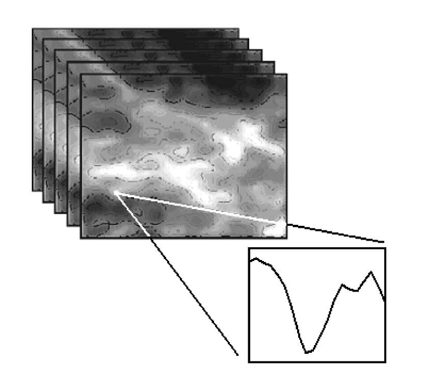
Figure 1: Velocity spectra extracted from a 21 cm data cube. Each velocity channel is an image of the HI gas at a given velocity.

Since the morphological characteristics of HI bubbles are very different from one bubble to another, their detection on a morphological basis is difficult. On the other hand, their dynamical characteristics are much more stable: the expansion velocity of bubbles associated to individual stars (and of radius of a few parsecs) are generally $\sim$ 10 km s^-1 (Gervais & St-Louis, 1999; Cappa & Herbstmeier, 2000). Hence, the two opposite sides of the shell have a typical maximum relative velocity of 20 km s^-1. In the CGPS HI cubes, this results, due to the Doppler shift, in a characteristic signature detectable in the velocity spectra (see Figure 1): two distinct peaks can be seen, one blueshifted and one redshifted, and separated by approximately 20 km s^-1. Our strategy is as follows: we seek first to detect expanding bubbles using their dynamical characteristics, hence by detecting the characteristic two-peaked profile in the velocity spectra associated with bubbles. Because this is a pixel-by-pixel approach, the bubble morphology is no more of prime importance, and we want to use it only afterwards, as a further confirmation to the detection. The presence of two peaks separated by 20 km s^-1 in a velocity spectrum is indeed not sufficiently restrictive to make a reliable bubble detection: much structural noise, for example velocity crowding on a line of sight or the presence of converging clouds, is likely to cause false shell detections. As will be seen, the morphology and other indicators are therefore used for confirmation. Also, we intend to first confine our survey to the Perseus Arm ($l=100^{\circ}$ to $140^{\circ}$) in order to avoid the confusion in the velocity-distance relation existing for $l<90^{\circ}$ and $l>270^{\circ}$. This way, we believe that a detector pointing to regions of space where dynamical characteristics of expanding shells are found performs a valuable cleaning of the data and significantly reduces the subsequent search field.

1.1 Expanding Structures and the Models of the ISM

The so-called bubbles, shells or cavities, referring to the ISM gas, are technically local lacks of gas with a boundary that is neutral or ionized and of variable density. Because of their expansion and of their often circular morphology, it is generally acknowledged that those objects result from a local momentum injection in the ISM. One of two important questions that can be asked refers to the nature of this energy source. The second question inquires about the effect those objects have on the structure of the ISM. Answering these questions is related more or less directly with the particular characteristics of the shells, which are deduced from observational data in a variety of spectral domains. Those characteristics are mainly: the mass of the shell, its expansion velocity, its dimensions, the density inside and outside of the bubble. Deriving those quantities from observational data allows one to confront them with hydrodynamical models of expanding bubbles in a given medium, which can be elaborated in relation to any plausible energy injection hypothesis and models of the ISM.

Neutral hydrogen is a major component of the galactic ISM (M_HI $\approx$ $2\times 10^{9}$ M_⊙). Field, Goldsmith & Habing (1969)’s pioneering work opened the way to the multi-phase models of the ISM. However, their initial model did not take into account violent events such as SN explosions. Those were considered by McKee & Ostriker (1977), who introduced the hot and ionized phase of the ISM (HIM for Hot Ionized Medium). This 3-phase model efficiently predicts the pressure, electron density and velocity dispersion of the ISM clouds, as well as the intensity of the soft X-rays emission of the ISM. The values of the filling factors are however less certain. McKee (McKee, 1995) and Cox (Cox, 1995; Cox & Smith, 1974) do not agree about the place taken by the HIM in the ISM : McKee believes the HIM makes up the intercloud medium, while Cox believes it has a small filling factor and is confined to dispersed bubbles. It is the determination of the HIM filling factor that will settle between the different ISM models - bringing the important link between the study of expanding shells and large scale modeling of the ISM. The HIM filling factor can only be determined from observational data.

Four categories of hypotheses can be proposed to explain the existence of expanding structures: 1) the sweeping of the ISM by the winds of massive stars (Lozinskaya, 1992; Oey, Clarke & Massey, 2001); 2) the progression of an ionization front followed by a recombination (McCray & Kafatos, 1987); 3) one or several SN explosions (Tenorio-Tagle & Palous, 1987); and 4) the collision of high velocity clouds of neutral gas with the disk of the Galaxy. The choice of the right hypotheses is difficult but determinant, since the astrophysical implications regarding the different ISM models derived from the existence of expanding objects are completely different in each of the four above cases. There exists no complete and general theory explaining all the aspects of the stellar winds and SN interactions with the ISM. Nevertheless, there are some simplified models that are able to explain the observations (Elmegreen & Lada, 1977; McCray & Kafatos, 1987; Lozinskaya, 1992).

What makes the choice of a model difficult is, firstly, that they are all incomplete, and secondly, that the observational data are too limited to supply enough typical cases to make a significant validation. This last point in itself clearly justifies our purpose: even if our automatic bubble detector could only find a few very regularly shaped objects, this would be an appreciable contribution to the discrimination of existing models of bubble formation and evolution. The high resolution of the CGPS makes it possible to visualize bubbles of radius down to a few parsecs in the Perseus Arm. Those are especially ill represented in the current database, and are thus not well studied even if they are less complex than large scale structures. Considering the extent of the CGPS field (666^∘2), the need of an automatic detector for expanding shells is obvious.

1.2 Proposed Strategy

Little work has been published on the automatic detection of expanding shells (Mashchenko, Thilker & Braun, 1999; Thilker, Braun, & Walterbos, 1998; Mashchenko & St-Louis, 2002), and their aim was mostly on the comparison of spherical structures observed in the velocity channels of HI data cube, with structures predicted by hydrodynamical simulations of expanding bubbles in the ISM. They are therefore limited to morphological recognition.

Our approach is to recognize the dynamical behavior of an expanding bubble, characterized by its velocity spectra. The 21 cm data collected by the CGPS contain HI abundance and kinematical information: as mentioned earlier, a characteristic dynamical profile can in principle be found in every velocity spectra extracted from every pixel of the bubble. This detection technique avoids the difficulties linked to the often distorted morphology of the bubbles. Bubbles are indeed hardly ever spherical and most often incomplete, which implies the subjectivity of a human observer and the difficulty of a purely morphological detection. Working with the velocity spectra allows a pixel-by-pixel evaluation of the likelihood of finding a bubble at a particular location in the data cube. Subsequent steps are to look for high concentrations of selected pixels in the data cube, and finally to consider the morphology of the detection, which is no longer the principal visual characteristic of an expanding HI shell.

The presence of two peaks separated by 20 km s^-1 in a velocity spectrum is unfortunately not sufficiently restrictive to make a reliable bubble detection. As will be discussed in sections 3 and 4, it is partly for this reason that we used an artificial neural network (ANN) for the first detection step. This tool is now often encountered in astrophysics, mostly as a classification device. We therefore present an overview of our ANN classifier in section 3, after the description of the CGPS data in section 2. In section 4 we expose the pixel-by-pixel detection method for the velocity spectra, while section 5 deals with the morphological validation of hypothesized bubbles. In section 6, the detector is performed on a simulated purely turbulent HI gas data cube. We present some preliminary results in section 7 before concluding in section 8.

2 The Data

Many 21 cm surveys of the Galaxy were accomplished in order to perform large scale study of the ISM: Heiles & Habing (1974), Weaver & Williams (1973), Colomb, Pöppel & Heiles (1980) and in particular the CGPS (Normandeau, 1996; Taylor, 1999; Higgs, 1999). The CGPS aimed at systematically observing the galactic plane, in the radio continuum and in the 21 cm HI line, between longitudes 75^∘ to 145^∘ and latitudes -3^∘ to 5^∘. This project is the result of contributions from Canadian university researchers and is carried out at the Dominion Radio Astrophysical Observatory (DRAO).

The synthesis telescope is a 7-antenna interferometer oriented east-west and with a maximum length of 604 m. This allows a $\sim$1.0’ resolution at 1420 MHz, while the previous large-scale HI surveys have resolution poorer than 4’. Each antenna is about 9 m in diameter, which gives a synthesized field of view of 2.5^∘ at 21 cm. Because of the 13 m minimum length of the interferometer, the minimum sampling resolution is $\sim$ 1^∘ at 21 cm. A 26 m antenna was used to observe the larger scales up to the survey dimensions. The total field covers 666^∘2 in 190 overlapped individual fields composing 36 5.12^∘ mosaics. Due to the primary beam of each antenna, the attenuation of the signal increases with the distance to the field center. This and the partial overlap of the individual fields causes the noise to vary in the final images. For this reason, a noise level map is supplied for each mosaic. Table 1 summarizes the parameters of the DRAO 21 cm HI data.

3 Artificial Neural Networks (ANNs)

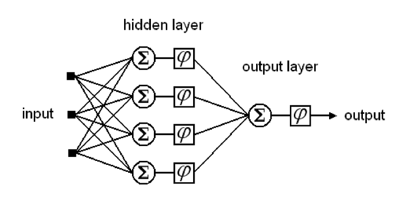
Figure 2: Schematic representation of a feedforward neural network. To each connection is associated a synaptic weight (the free parameters). A neuron first computes the weighted sum of its synaptic connections before applying a usually non-linear transfer function $\varphi$ to produce an output. The dimensions of the input and output spaces are at the user’s discretion. In this paper, the input vector (the input data) is a 12-component segment of a velocity spectrum, and the output is a one-dimensional degree of membership to the class of expanding bubbles.

An ANN is a network of many simple parallel operating elements (see Figure 2). This configuration is inspired by the way biological neurons effectively communicate: neurons located in successive layers are massively interconnected by synaptic connections allowing electric signal transmissions. One neuron thus collects signals from many neighbors, and every signal is weighted by the efficiency of the synaptic connection that is involved. Learning can be defined technically as the process of reinforcement and inhibition of those connections, in order to create a neural network appropriate to the task to be learned. In the case of ANNs, a free parameter called the synaptic weight stands for the connection efficiency.

A schematic representation of an example of a feedforward neural network is showed in Figure 2. This network has a three-dimensional input space, one hidden layer containing four neurons, and its output layer contains one neuron - the output space is one-dimensional. The neurons are represented as summation signs because they compute the weighted sum of their synaptic connections. To each connection is associated a synaptic weight, which is an adjustable free parameter. The dimensions of the input and output spaces, as well as the hidden layers dimensions, must be determined by the user.

3.1 The Backpropagation Algorithm

ANN learning consists in the adjustment of all the synaptic weights of all the connections, until a satisfactory mapping is achieved. The so-called supervised learning of an ANN consists in feeding the network with a training set of input-output mappings $(\vec{x}(n),\vec{d}(n))$, where $\vec{d}(n)$ is the desired output for the $n$th input vector $\vec{x}(n)$. After each presentation, the ANN error is computed and is used to adjust the free parameters, so that the error will be minimized if the same situation is encountered. The learning process consists of adjusting all the weights, so that at each iteration the network is heading for the direction of the more negative gradient on the error surface. The usual learning algorithm used to achieve this iterative minimization is called the backpropagation algorithm, because the error at the network output is propagated backward through the layers in order to calculate the proper adjustment for each weight in each layer.

The backpropagation algorithm updates the weights for each neuron, beginning with the output layer. Let $e_{j}(n)$ be the observed error at the output neuron $j$ for the training datum $n$:

$$e_{j}(n)=d_{j}(n)-y_{j}(n)$$ (1)

where $d_{j}(n)$ is the desired output for neuron $j$ and $y_{j}(n)$ ) is the observed output. The goal is to minimize $E(n)$, the sum of the mean square errors (MSE) observed on the set of $C$ output neurons for the training datum $n$:

$$E(n)=\frac{1}{2}\sum_{j\epsilon C}e_{j}^{2}(n)$$ (2)

The output of neuron $j$ is defined by:

$$y_{j}(n)=\varphi[v_{j}(n)]=\varphi[\sum_{i=1}^{r}w_{ji}(n)y_{i}(n)]$$ (3)

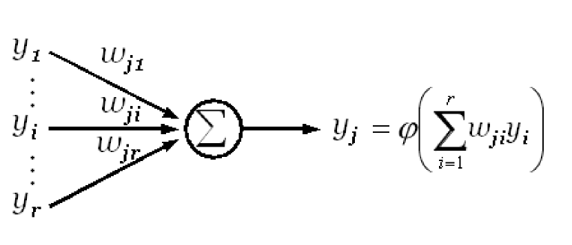
Figure 3: The neuron $j$ in the output layer sums the weighted outputs of the neurons $i=[1,r]$ of the preceding layer. The transfer function $\varphi$ is then performed to produce the neuron $j$ output $y_{j}$.

where $\varphi[.]$ is the neuron transfer function (a usually nonlinear function in order to produce a nonlinear mapping), $v_{j}(n)$ is the weighted sum of the neuron $j$ inputs, $w_{ji}(n)$ is the connection weight between the neuron $i$ in the preceding layer (containing $r$ neurons) and the neuron $j$ in the output layer, and $y_{i}(n)$ is the neuron $i$ output - see Figure 3.

To minimize $E(n)$, the weight $w_{ji}(n)$ must be updated in the direction in which the error gradient $\frac{\partial{E(n)}}{\partial{w_{ji}(n)}}$ is decreasing:

$$\triangle{w_{ji}}(n)=-\eta{\frac{\partial{E(n)}}{\partial{w_{ji}(n)}}}$$ (4)

where $0\leq\eta\leq 1$ is the learning rate. The chain rule gives:

$$\triangle{w_{ji}}(n)=-\eta{\frac{\partial{E(n)}}{\partial{w_{ji}(n)}}}=\eta\delta_{j}(n)y_{i}(n)$$ (5)

$$\delta_{j}(n)=e_{j}(n)\phi^{\prime}_{j}$$ (6)

where $\delta_{j}(n)$ is called the local gradient of the error surface.

The case of the hidden layers is similar, but the local gradient of the neuron $j$ is now function of all the local gradients of the neurons $k$ in the layer following the one who’s neuron $j$ is being updated:

$$\delta_{j}(n)=\phi^{\prime}_{j}\sum_{k\epsilon C}\delta_{k}(n)w_{kj}(n)$$ (7)

3.2 Classification with ANN

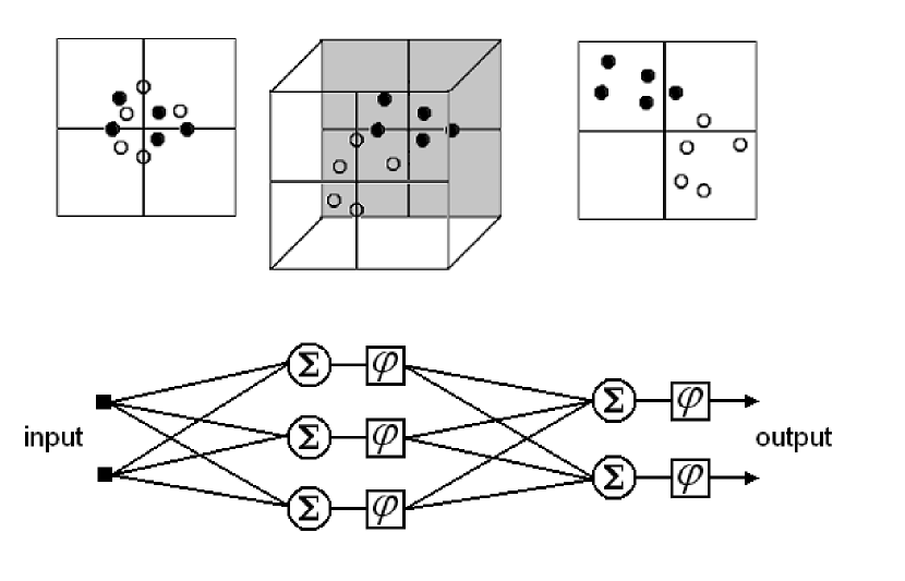
Figure 4: Mapping of data from an input space into an output space, in order to achieve a classification. The ANN 3-neuron hidden layer acts as a 3-dimensional intermediate space allowing the separation of intricate data.

An ANN may be described as an algorithm that maps data, from an input space into a user-chosen output space. Among other possibilities, mapping a data set into an output space having meaningful categories is equivalent to classification. Figure 4 illustrates the classification of data by mapping the input set into a higher dimensional intermediate space, permitting the separation of two categories. The data are afterwards mapped into the output space as separated sets, or classes. It is this particular application of the ANNs that we want to take advantage of for this pattern recognition task in the velocity spectra.

One interesting thing is the generalization capability of the ANN, which can interpolate between new and unknown input data. This generalization ability, as well as the speed of the convergence and the final ANN global performance, crucially depends on the training set. For all the eventual input data to be properly represented in the output space, the training set must cover most of the space. It must include as various examples as possible, and cover equally the different cases that may be encountered while using the trained ANN. A very common case in the training set will be very well delimited in the output space, while a rare one could be associated to some other class or be bluntly treated as noise.

The main distinction between ANNs and more classical classifiers, such as cross correlation, is thus the determination of the classification criteria. A classical classifier needs precise criteria that are sufficient to make a distinction between classes. Those criteria are initially known and chosen by the user, hence they must have a known signification, or at least be empirically identified and accessible. To use an ANN classification, one only requires a good and representative training set. The ANN will, in a way, choose its classification criteria by itself, by adjusting its synaptic weights. The only known conditions are the ANN configuration (number of layers, number of neurons, transfer functions) and the initial values of the free parameters. The only a priori “criterion” is the error minimization algorithm. What is obtained is therefore a totally empirical classification, with no a priori statistical model.

This last point may cause some uneasiness: the fact that the ANN chooses the distinction criteria may be seen as a loss of control on the part of the user. An ANN could choose criteria that are entirely irrelevant to the user’s purpose, and consequently it would be unable to process other data than the ones of the training set. On the other hand, when intuitive criteria are not available or are not sufficiently restrictive to achieve a good classification, an ANN may be able to isolate hidden characteristics and use them to make relevant decisions. Moreover, its generalization ability allows the recognition of distorted and noisy data, that a classical classifier might not be able to process.

These last two points justify our use of an ANN for the detection of the kinematical signature of expanding HI bubbles. Another classifier could have been used, but based on uncertain classification criteria: for example, cross-correlation would require a spectral template that we do not possess. Indeed, the search of a profile with peaks separated by 20 km s^-1 is not sufficiently restrictive. Our detector is thus required to find other criteria to recognize the bubbles’ velocity spectra. The data are furthermore noisy - in addition to the detection noise, we have to deal with structural noise: the expanding shells evolve in a HI environment made of clouds of various sizes, of filaments, and other various structures that disturb the spectra. We believe that an ANN classifier may be more likely than any other classifier to integrate a sufficiently general and restrictive model of an expanding bubble velocity profile, in order to recognize it amongst all other structures, and despite the noise.

There are several possible ANN configurations. We chose a multilayer perceptron (MLP), which is a feedforward neural network such as the one described by Figure 2, because it proved its value in many practical classification problems, and also because it does not make any a priori assumption about data distribution, contrary to other statistical classifiers. The main shortcoming of the MLP in this particular context is that it may take decisions about regions of space that were not covered by the training set. The MLP will not reject a case pleading incompetence. Independent rejection criteria allowing to discard some of the MLP decisions will be described in sections 4 and 5.

The main difficulty of our proposal is about the training set. The small number of known certified observational bubbles makes it difficult to assemble a set of diversified and representative examples. This certainly requires special attention, as will be discussed later.

For more details about the theory and implantation of ANNs, the reader can consult: Haykin (1998), Demuth & Beale (2000), Principe, Euliano & Lefebvre (2000).

4 Dynamical Detection

The detection of the dynamical characteristics of a bubble in the velocity spectra is a pixel-by-pixel one: the goal is to assign a degree of confidence to each pixel, expressing how much the corresponding velocity spectrum matches the dynamical profile that is looked for. This first step is taken care of by a MLP with two hidden layers (the layers between the input and output layers) containing 17 and 2 neurons, respectively. The error minimization is performed by a Levenberg-Marquardt backpropagation algorithm, which is a faster variation of the standard backpropagation algorithm exposed in section 3 (Hagan & Menhaj, 1994). The learning rate is 0.17. Those conditions allow to reach a good MLP performance (mean square error (MSE) $\leq$ 0.014) in a relatively short period of time. The MATLAB Neural Network Toolbox has been used.

Too long a training can compromise the MLP generalization capability: the worst limit is the MLP having learned to recognize each individual training spectrum, and being unable to recognize any other similar spectrum that is unknown. A standard cross-validation technique that averts overtraining is the use of a validation set, which is a data set composed as the training set, but that is not used for the training itself. The MLP performance is computed for each iteration over the validation set, and the training is stopped when the error over the validation set begins to rise. The training set contains $\sim$1300 spectra and the validation set $\sim$200. This ratio is standard.

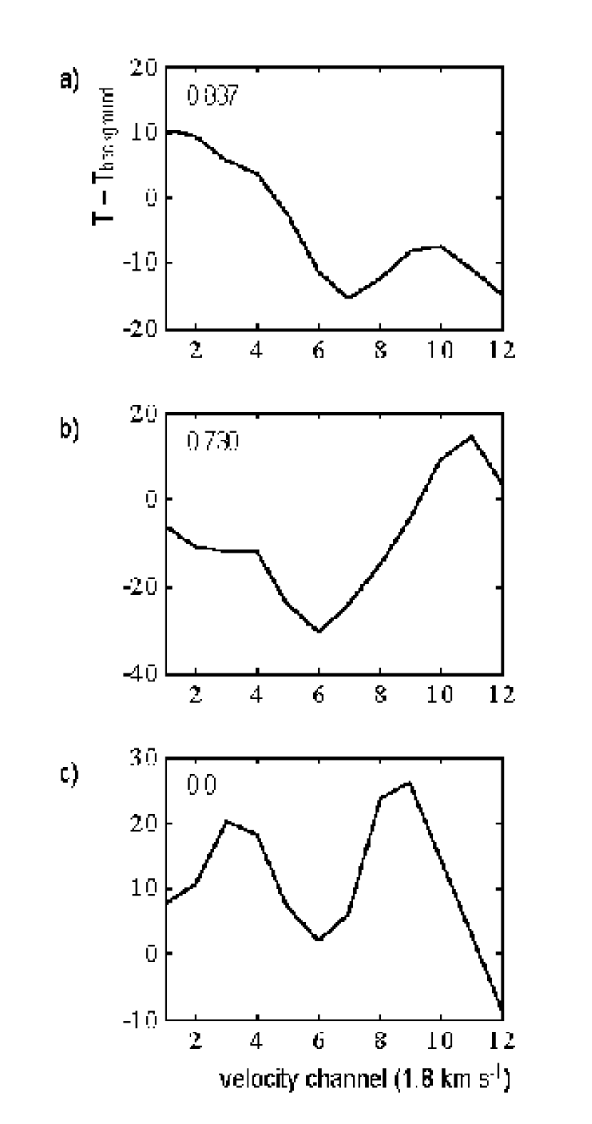
Figure 5: Three velocity spectra. The MLP output is indicated on each graph. a) Spectrum effectively positive and detected as such (belongs to GSH138-01-094); b) Negative spectrum, insufficient MLP output; c) Negative spectrum, insufficient MLP output.

The vectors presented at the input layer of the MLP are 12-channel segments of the velocity spectra. This number of channels spans $\sim$20 km s^-1, a velocity interval sufficient to contain the dynamical profile of the bubble. The background (an average spectrum over the whole data cube) is subtracted beforehand, in order to filter the irrelevant global characteristics such as the local diffuse material associated with the spiral arm. Only the local HI enhancements and dynamical characteristics (such as an expanding bubble) are preserved. The MLP output is a number in the range [0, 1] expressing how good the 12-channel segment matches the dynamical profile of an expanding bubble. Figure 5 shows examples of spectra classified by the MLP. Even if the three examples show a two-peaked profile, the MLP output is different for each. Some information that is not directly accessible or intuitive, but that allows some discrimination, is therefore extracted by the MLP.

The results presented in this paper were obtained with a committee of 4 MLPs. We simply averaged the results coming from each of the 4 networks. The MLPs were trained over velocity spectra taken from 6 different data cubes, each of which containing one known bubble.Two of those bubbles are artificial bubbles: spheres of relatively high brightness temperatures have been added in real and otherwise unaltered HI data cubes. This is a way to enrich and improve the training set by making it more representative: even though those two bubbles are not real, inserting them into the training set introduces representative dynamical characteristics inside various HI environments, and thus contributes to enrich knowledge of the MLP. The 4 real bubbles are: G132.6-0.7-25.3; the bubble related to WR144 (galactic coordinates 80.04+0.93-26.2); the bubble related to WR139 (76.6+1.43-69.07); and the bubble related to WR149 (89.53+0.65-66). The MLP performance will naturally get better as the training set will be enriched with new bubble instances.

As mentioned in section 3.2, a MLP is not well suited for rejecting data: it will output a decision for every input datum, even if it is unable to make a proper classification given the experience acquired during its training. The MLP taken alone may thus make an important number of false detections: generally, 2% to 10% of the pixels are incorrectly identified “bubble” in the whole data cube. A filtering is therefore performed by verifying a number of conditions in each selected spectrum. By comparing our known examples of positive spectra (spectra belonging to known bubbles), we have been able to isolate some discriminant features most of them have in common. However, the negative spectra may have every possible shapes, and occasionally present some of these features. For this reason, we rather identify rejection criteria, allowing us to exclude a detection made by the MLP. These conditions are supplied by statistics compiled over all the positive cases we have. Those characteristics are very pragmatic, such as the values and positions of the spectrum extrema. Applying those rejection criteria on the MLP detections allows us to exclude a significant part of the false detections, but keeps most of the correct ones.

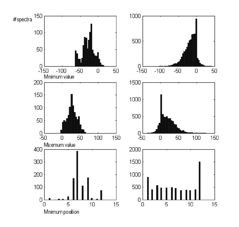
Figure 6: Histograms illustrating the statistics of 3 visual features in positive (left hand side) and negative (right hand side) spectra sets. Downward : the value of the minimum; the value of the maximum; the position of the minimum.

Figure 5 a) illustrates a typical positive spectrum which shows some positive visual characteristics:
$\bullet$ The minimum position is between channels 6 and 9;
$\bullet$ The minimum value is $<$ -12 (negative values are due to the background subtraction);
$\bullet$ The maximum value is $>$ 0.
The approximately central position of the minimum is a quite intuitive feature that depends directly on the dynamics of expanding bubbles. However, the values of the extrema (which are brightness temperatures relative to the average background) depend on physical conditions that are less stable, such as the ratio between the shell and ambient medium densities. In fact, the rejection conditions were chosen on purely empirical basis: we only noticed they could make some distinction between a positive set and a negative set. Figure 6 shows the statistics of the 3 characteristics stated above, to visually compare positive and negative sets. One can notice some trend for the positive sets. If some permitted intervals are established for each condition, an important part of the false detections can be rejected. In the examples presented in section 7, we simply established lower and upper limits such that 88% of the spectra of the positive histograms are preserved.

5 Morphological Detection

We believe the pixel-by-pixel dynamical detection is helpful to begin the search because of the difficulties arising from a morphological detection in several successive velocity channels. This first step taken, we are left with a cube in which patches of positively identified pixels are found. In a single velocity channel, this results in connected objects, or “blobs”, of various dimensions and shapes.

5.1 The Dimensions of the Object

The object dimension in pixels depends on its intrinsic dimension and on its distance. As a velocity channel is associated to a galactocentric distance, it is possible to establish a lower limit, function of the velocity channel, to the number of pixels corresponding to a blob of a few parsecs diameter, and thus necessary for a blob to be a real bubble. The higher limit for the bubbles’ size is indirectly determined by the dynamically based detection, since the maximum expansion velocity for bubbles of a few parsecs is typically 10 km s^-1.

5.2 The Object Shape

One should keep in mind that the blobs with which we now have to work are in fact concentrations of positive detections - that is to say, their shape do not necessarily match the visual shape of the bubble. Despite this fact, it is clear that a concentration of detections having a roughly circular and condensed shape is more likely to be a bubble, than some very elongated and sharp filament. It is thus relevant, at this point, to take morphology into account.

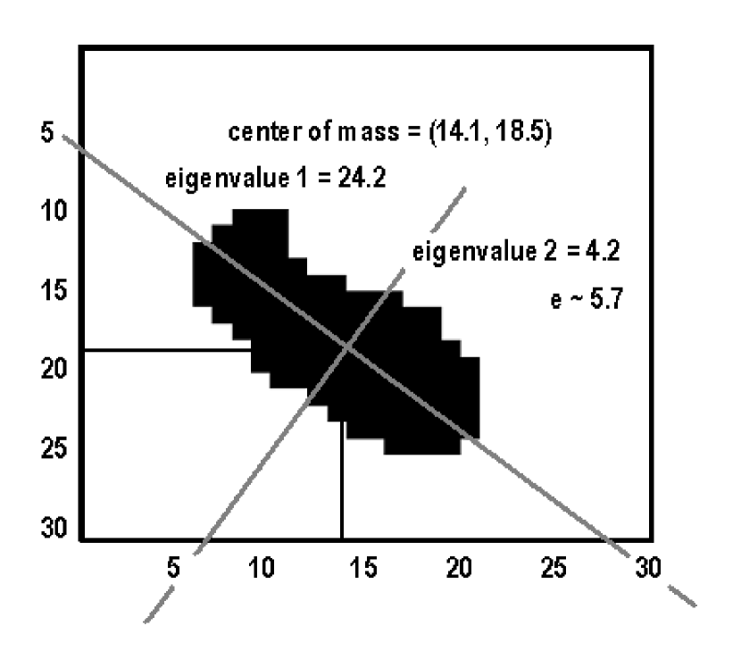
Figure 7: Characterization of a blob by its association with an ellipse. The ellipse eccentricity is estimated by the ratio of the eigenvalues of its 2 principal axis.

To begin with, the size and orientation of the object are characterized using a principal component analysis: the directions of the two principal axis of the blob are calculated, and the eccentricity of an associated ellipse is estimated by the ratio of the eigenvalues of the axis (see Figure 7). A new rejection criteria is then defined based on a superior limit to the eccentricity.

5.3 Increasing Intensity Criterion

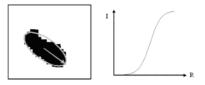
Figure 8: The increasing intensity criterion : the HI abundance must increase with the bubble radius. What is effectively verified is that the pixels intensity on the ellipse principal axis increases as we progress away from the blob center. This “center” is not the center of mass but the minimum of the intensity neighboring the center of mass.

Because an HI bubble corresponds to a local lack of gas, another rejection criterion for a given velocity channel, directly linkable to the physics of the phenomenon, and independent of the dynamics or morphology, is the fact that the intensity of the 21 cm emission should increase in a radial fashion around its center (see Figure 8).

6 Turbulence: Simulation of self-similar HI in the Perseus arm

As mentioned earlier, the structural noise due to various structures in HI may cause false detections. Apart from the rejection criteria and the morphological confirmation just exposed, there is not much to be done against it. It is however of interest to verify if our detector could be tricked by turbulence alone. We performed our detector on a simulated purely turbulent HI gas data cube such as described below. The subsequent rejection criteria on the velocity spectra were not used, because the brightness temperatures relative to the average background could not be consistent in real and simulated cubes. The committee of MLPs does retain some spectra as positive, but those detections do not pass the morphological test: in fact, no blob at all can be isolated, the maximum number of connected pixels in a concentration of positive detections being 18 ($\sim$$\frac{1}{4}$ of minimum number accepted by the detector).

The rest of this section describes how we have simulated the spectro-imagery observation of the observed part of the Perseus arm on the hypothesis that the HI density structure and kinematics are only due to turbulence and Galactic rotation. In this section we describe how we modelled the HI 3D density and velocity fields and how we constructed the spectro-imagery observation from these.

We consider that the center of the Perseus arm is at a distance of 2 kpc from the Sun and that its depth is 0.3 kpc. As the field observed at DRAO is $2.6^{\circ}\times 2.6^{\circ}$, this translates into a surface of $\sim 0.1\times 0.1$ kpc at the Perseus arm distance. To simulate the Perseus arm we have produced a $128\times 128\times 384$ box that represents the observed portion of the Perseus arm ($0.1\times 0.1\times 0.3$ kpc). Each cell in that box has a linear size of 0.75 pc.

6.1 The 3D velocity field

The simulated 3D velocity field ($v(x,y,z)$) is the sum of the Galactic rotation component ($V(x,y,z)$) and of a turbulent component ($\delta v(x,y,z)$). To lighten the text, we drop the $(x,y,z)$ in the following.

6.1.1 The Galactic rotation velocity component

To simulate the Galactic rotation velocity component, we proceeded as follows. Each point in the simulated cube has been attributed a longitude $l$, latitude $b$ (corresponding to our DRAO observation) and a distance from the sun (the center of the box being at 2 kpc). The Galactic radius $R$ of each cell element is then given by:

$$R=(D\cos(l)-R_{\odot})/\cos(\theta)$$ (8)

where

$$\theta=\tan^{-1}\left(\frac{D\sin(l)}{D\cos(l)-R_{\odot}}\right)$$ (9)

with $R_{\odot}=8.5$ kpc.

Following Burton (1992), the Galactic angular velocity $\Omega$ has been estimated to be:

$$\Omega=\Omega_{\odot}(1.0074*(R/R_{\odot})^{0.0382}+0.00698)$$ (10)

with $\Omega_{\odot}=220$ km s^-1. Finally the angular velocity component along the line of sight is given by the following expression:

$$V=(\frac{R_{\odot}}{R}\Omega-\Omega_{\odot})\times\sin(l)\cos(b).$$ (11)

6.1.2 The turbulent velocity component

To simulate the self-similar properties of the velocity structure we have used 3D fractional Brownian motion simulations (Stutzki et al., 1998; Miville-Deschênes et al., 2003). We have simulated a $128\times 128\times 384$ cube with spectral index -11/3, to simulate Kolmogorov type turbulence. The average of the turbulent velocity field was set to zero ($<\delta v>_{x,y,z}=0$) and its dispersion to 20 km s^-1.

6.2 The density field

The simulated 3D density field ($n(x,y,z)$) was also built using a fractional Brownian motion simulation with a spectral index of -11/3. No correlation between velocity and density was introduced. We have subtracted the minimum value from the 3D density cube to allow only positive density values. Because of the relatively small size of the observed region, we did not introduce any variation of the average density with the height above the Galactic plane.

6.3 Building the spectro-imagery observation

The spectro-imagery observation (also called position-position-velocity or PPV cube) has been constructed by making the assumption that every gas cell on the line of sight emits a thermally broaden Gaussian ($\sigma=\sqrt{k_{B}T/m}$) centered at $v(x,y,z)=V(x,y,z)+\delta v(x,y,z)$ and of amplitude $n(x,y,z)$ (see Miville-Deschênes et al. (2003) for the details). We have considered optically thin Cold Neutral Medium gas at $T=100$ K. We have constructed a $128\times 128\times 128$ PPV cube that gives the column density on each line of sight and at each velocity $u$ (velocity bin is 1.65 km s^-1) using the following equation:

$$N_{H}(x,y,u)=\alpha\sum_{z}n(x,y,z)\exp\left(-\frac{[u-v(x,y,z)]^{2}}{2\sigma^{2}}\right).$$ (12)

Here $\alpha$ is a normalization factor that takes into account the spectral resolution and the linear size of a cell along the line of sight.

7 Preliminary Results

The two test cubes have galactic coordinates ($\Delta$l; $\Delta$b; $\Delta$v) = (136.75, +139.30; -0.10, -2.65; +12.6, -136.7) and ($\Delta$l; $\Delta$b; $\Delta$v) = (73.1, 75.7; +0.25, +2.9; +60.7, -102.9), and contain respectively bubbles GSH138-01-094 and G73.4+1.55. Those two bubbles were not used for the MLP training, therefore the detector possesses no preliminary knowledge of those particular cases. It is believed that GSH138-01-094 could have been caused by a SN (Stil & Irwin, 2001), while G73.4+1.55 is linked to WR134 (Gervais & St-Louis, 1999).

It took a few hours to train the MLPs, and their MSE on the validation set is $\leq$ 0.014. The detection itself on a cube of 128x128x79 12-channel spectra takes $\sim$ 5 minutes with a Pentium 4, 1.9 GHz and 512 Mo ram.

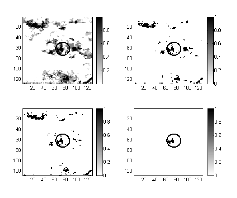
Figure 9: Results of the detection of GSH138-01-094. The ellipse indicates the bubble location and scale at its maximum expansion. From left to right, downward : the MLP detection; after a 0.82 threshold; after application of the rejection criteria on the spectra; after application of the rejection criteria on the blobs.

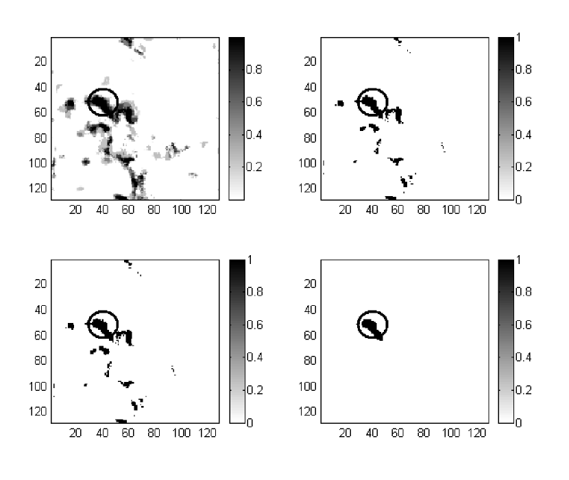
Figure 10: Results of the detection of G73.4+1.55.

Figure 9 shows the velocity channel corresponding to v $\approx$ -94 km s^-1, where GSH138-01-094 should be detected, through the stages of the detection. Figure 10 shows the same stages for G73.4+1.55, at v $\approx$ -11.4 km s^-1. Table 2 traces the evolution of the amount of false detections for each step, in pixel percentages and in number of preserved blobs.

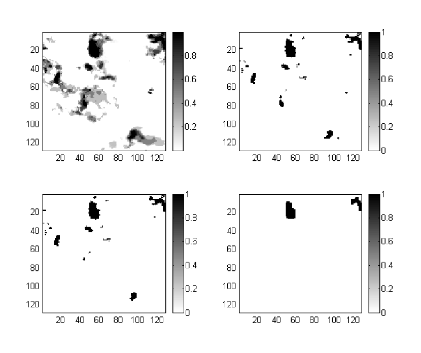
Figure 11: Detection at coordinates (l,b,v) = (138, -0.5, -7). Corresponds to the location of an unknown bubble, at least visually convincing in its morphology as well as in its dynamics.

Figure 11 shows a detection at (l,b,v) $\sim$ (138, -0.5, -7) in the same data cube where GSH138-01-094 is found. The presence of a bubble is visually very convincing, as much in its morphology through successive velocity channels, as in its dynamical signature in the velocity spectra. It would certainly be relevant to check the eventual presence of a WR star or a supernova remnant at this location.

7.1 Discussion

0.5% to 0.7% of the detections, or less than 30 to 60 blobs, do not correspond to any known bubbles. It is however tempting to verify those false detections in the hope of finding out that some of them were justified. What we want to point out is that, even if our detector gives several false alarms, those very limited and confined regions of the sky constitute a search field considerably reduced compared to the whole sky. The purpose of our detector is not to make a final decision about the validity of a detected bubble, but to raise flags in order to guide the researchers towards regions of the sky with relatively high probability of finding one.

8 Conclusion

The next step to this work is to use the detector on a large section of the CGPS HI data. The eventual new cases of bubbles found using the detector will be integrated to the MLP training set in order to improve its specialization. For the first time, an evaluation of the amount and distribution of expanding bubbles of a few parsecs radius will be possible.

Such an evaluation is critical to evaluate the relative importance of the HIM in the ISM, which is traditionally addressed in terms of the porosity parameter $Q$. This parameter is defined as the ratio between the volume occupied by the bubbles in the Galaxy and the total volume of the Galaxy. $Q$ is thus directly related to the HIM filling factor, if we suppose that the HIM fills the bubbles (McKee & Ostriker, 1977). For example, Oey & Clarke (1997) deduced $Q$ from an analytical expression of the distribution and size of bubbles and superbubbles. If their prediction for a maximum in the HI cavities radii distribution was verified, this would constitute a new constraint for the SN remnants evolution, for the ISM conditions and for the typical energy injected by SN in galaxies. However, an observational verification of this prediction in the small radii regime is not possible because of the lack of known cases. Our results could help to clarify this issue.

In this paper, it has been shown that a detector using the dynamical features in the velocity spectra of HI data cubes can point out zones where there is a relatively high probability of finding an expanding bubble. This detector is based on the classification of a MLP, and on some independent dynamical and morphological rejection criteria. The test bubbles have been correctly detected with a false detections percentage of $\sim 0.6\%$, which significantly reduces the subsequent search field. This preliminary cleaning could be followed by a human inspection or other more complex automatic analysis processes, which could be applied on a few objects rather than a vast amount of rough data.

Table 1: Parameters of the CGPS 21 cm survey (Higgs, 1999).

Parameter	Value
Survey
Number of Synthesis Telescope Fields	190
Field Dimensions (∘)	2.5
Spacing of Field Centers (∘)	1.86
Spatial Resolution	1.0’x1.0’$\csc\delta$
Number of Velocity Channels	272
Spectral Resolution (km s-1)	1.319
Channel Separation (km s-1)	0.82446
RMS Noise (Field Center) (K)	2.9
Mosaics
Number of Mosaics	36
Size of Mosaics (∘)	5.12 x 5.12
Overlap of Mosaics (∘)	1.1
Area Covered (∘2)	666
Galactic Longitude Coverage (∘)	74.2 to 147.3
Galactic Latitude Coverage (∘)	-3.6 to 5.6

Table 2: Evolution of the False Detections Through the Detection Stages.

Stages of the Detection	GSH138-01-094		G73.4+1.55
	% False Detections(pixels)	# Preserved Blobs	% False Detections(pixels)	# Preserved Blobs
Threshold of 0.8	2.3	375	3.0	475
After Filtering the Spectra	1.9	305	2.7	456
After Filtering the Blobs	0.5	29	0.7	57

References

- Burton (1992) Burton, W. B., 1992, in The Galactic Interstellar Medium, edited by P. Pfenniger and P. Bartholdi, Heidelberg: Springer, p. 1
- Cappa & Herbstmeier (2000) Cappa, C. E., Herbstmeier, U., 2000, AJ, 120, 1963
- Colomb, Pöppel & Heiles (1980) Colomb, F. R., Pöppel, W. G. L., Heiles, C., 1980, A&A supp., 40, 47
- Cox (1995) Cox, D. P., Problems with the Diffuse Interstellar Medium, ASP Conference Series, Volume 80, Editor(s), A. Ferrara, C.F. McKee, C. Heiles, P.R. Shapiro.; Publisher, Astronomical Society of the Pacific, San Francisco, California, 1995.
- Cox & Smith (1974) Cox, D. P., Smith, B. W., 1974, ApJ, 189, 105
- Demuth & Beale (2000) Demuth, H., Beale, M., 2000, Neural Network Toolbox, For Use with MATLAB, User’s Guide, Version 3.0, The Mathworks
- Elmegreen & Lada (1977) Elmegreen, B. G., Lada, C. J., 1977, ApJ, 214, 725
- Field, Goldsmith & Habing (1969) Field, G. B., Goldsmith, D. W., Habing, H. J., 1969, ApJ, 155, 149
- Gervais & St-Louis (1999) Gervais. S., St-Louis, N., 1999, AJ, 118, 2394
- Hagan & Menhaj (1994) Hagan, M. T., Menhaj, M., 1994, IEEE Transactions on Neural Networks, 5, 989
- Haykin (1998) Haykin, S. S., 1998, Neural Networks, a Comprehensive Foundation, Prentice Hall, 2nd edition, 842pp.
- Heiles & Habing (1974) Heiles, C., Habing, H. J., 1974, A&A supp., 14, 1
- Higgs (1999) Higgs, L. A., 1999, ASPCS, 168, 15
- Lozinskaya (1992) Lozinskaya, T. A., 1992, SNe and Stellar Wind in the Interstellar Medium, American Institute of Physics, New York, 467pp.
- Mashchenko, Thilker & Braun (1999) Mashchenko, S., Thilker, D. A., Braun, R., 1999, A&A, 343, 352
- Mashchenko & St-Louis (2002) Mashchenko, S., St-Louis, N., Automatic Shell Detection in CGPS Data, ASP Conference Proceedings, Vol. 260, editors Anthony F. J. Moffat and Nicole St-Louis, San Francisco: Astronomical Society of the Pacific, 2002, p.65.
- McCray & Kafatos (1987) McCray, R., Kafatos, M., 1987, ApJ, 317, 190
- McKee & Ostriker (1977) McKee, C. F., Ostriker, J. P., 1977, ApJ, 218, 148
- McKee (1995) McKee, C. F., The Multiphase Interstellar Medium, ASP Conference Series, Volume 80. Editor(s), A. Ferrara, C.F. McKee, C. Heiles, P.R. Shapiro.; Publisher, Astronomical Society of the Pacific, San Francisco, California, 1995, p.292.
- Miville-Deschênes et al. (2003) Miville-Deschênes, M. A., Levrier, F. & Falgarone, E., 2003, ApJ accepted
- Normandeau (1996) Normandeau, M., 1996, The Galactic Plane Survey Pilot Project, PhD thesis, University of Calgary
- Oey & Clarke (1997) Oey, M. S., Clarke, C. J., 1997, MNRAS, 289, 570
- Oey, Clarke & Massey (2001) Oey, M. S., Clarke C. J., Massey, P., 2001, in Dwarf Galaxies and their Environment Conf. Proc., Klaas S. De Boer, Ralf-Juergen Dettmar, and Uli Klein editors, p.181
- Principe, Euliano & Lefebvre (2000) Principe, J.C., Euliano, N. R., Lefebvre, W. C., 2000, Neural and Adaptive Systems: Fundamentals throught Simulation, John Wiley & Sons, Inc.
- Stil & Irwin (2001) Stil, J. M., Irwin, J. A., 2001, ApJ, 563, 816
- Stutzki et al. (1998) Stutzki, J., Bensch, F., Heithausen, A., Ossenkopf, V. & Zielinsky, M., 1998, A&A, 336, 697
- Taylor (1999) Taylor, A. R., Radio Continuum Results from the Canadian Galactic Plane Survey, ASP Conference Series 168, Edited by A. R. Taylor, T. L. Landecker, and G. Joncas. Astronomical Society of the Pacific (San Francisco), p.3.
- Tenorio-Tagle & Palous (1987) Tenorio-Tagle, G., Palous, J., 1987, A&A, 186, 287
- Thilker, Braun, & Walterbos (1998) Thilker, D.A., Braun, R., Walterbos, R. M., 1998, A&A, 332, 429
- Weaver & Williams (1973) Weaver, H. F., Williams, D. R., 1973, A&A supp., 8, 1