Atomic Calculations and Spectral Models of X-ray Absorption and Emission Features From Astrophysical Photoionized Plasmas

Abstract

We present a detailed model of the discrete X-ray spectroscopic features expected from steady-state, low-density photoionized plasmas. We apply the Flexible Atomic Code (FAC) to calculate all of the necessary atomic data for the full range of ions relevant for the X-ray regime. These calculations have been incorporated into a simple model of a cone of ions irradiated by a point source located at its tip (now available as the XSPEC model PHOTOION). For each ionic species in the cone, photoionization is balanced by recombination and ensuing radiative cascades, and photoexcitation of resonance transitions is balanced by radiative decay. This simple model is useful for diagnosing X-ray emission mechanisms, determining photoionization/photoexcitation/recombination rates, fitting temperatures and ionic emission measures, and probing geometrical properties (covering factor/column densities/radial filling factor/velocity distributions) of absorbing/reemitting regions in photoionized plasmas. Such plasmas have already been observed in diverse astrophysical X-ray sources, including active galactic nuclei, X-ray binaries, cataclysmic variables, and stellar winds of early-type stars, and may also provide a significant contribution to the X-ray spectra of gamma-ray-burst afterglows and the intergalactic medium.

1 Introduction

With the launch of the X-ray satellites Chandra (Weisskopf et al. 2002) and XMM-Newton (Jansen et al. 2001; den Herder et al. 2001), high-resolution X-ray spectroscopy of diverse astrophysical objects has now become routine. X-rays, due to their origin in extreme astrophysical environments as well as their significant penetrating ability, can potentially provide a wealth of information about these sources. Their penetration power, in particular, implies that X-ray emitting plasmas are often optically thin. In such cases, complicated radiative transfer is negligible, allowing for particularly simple astrophysical models.

There are two main types of X-ray line-emitting plasmas: (1) Hot plasmas, which are mechanically heated through collisions and therefore have temperatures comparable to the observed line energies, and which produce X-ray line emission predominantly through radiative decay following electron impact excitation (hereafter, “collision-driven”), and (2) Photoionized plasmas, which are irradiated by a powerful external source and have subsequently lower temperatures consistent with photon heating (including both photoelectric and Compton heating), and which produce X-ray line emission through recombination/radiative cascade following photoionization, and radiative decay following photoexcitation (hereafter, “radiation-driven” or “photoionized”). Hot plasmas are produced in the coronae of stars (including the Sun), in shock-heated environments (such as supernovae, cataclysmic variables, and stellar winds of early-type stars), and in the intracluster media of clusters of galaxies. Photoionized plasmas have recently been unambiguously confirmed in X-ray binaries (Liedahl & Paerels 1996, Cottam et al. 2001), AGN outflows (Sako et al. 2000, Kinkhabwala et al. 2002), cataclysmic variables (Mukai et al. 2003), and even in the stellar wind of the WR+O binary $\gamma$ Velorum (Dumm et al. 2002). Hybrid plasmas, in which both collision-driven and radiation-driven processes are important, can also exist. So far, hybrid X-ray-line-emitting plasmas have not yet been unambiguously detected in any astrophysical source, but they are expected to play an important role in accretion disks, for example, which are strongly irradiated (implying radiation-driven processes are important) but also have high densities (implying collision-driven processes are important as well). Finally, we note that the mechanisms driving X-ray emission (either collision-driven or radiation-driven) in the two vastly different regimes of gamma-ray-burst (GRB) afterglows and the intergalactic medium (IGM) are still largely unknown. GRB afterglows may harbor hot plasmas produced through shocks and/or photoionized plasmas located in the ejecta or surrounding interstellar medium and powered by radiation from the burst and afterglow radiation. Similarly, the IGM may harbor hot plasmas from shocks due to structure formation and/or photoionized plasmas powered by radiation from active galactic nuclei (AGN) or starbursts.

Calculations of X-ray line emission from hot, collision-driven plasmas have been discussed in great detail by several authors, including Raymond & Smith (1977), Mewe, Gronenschild, & van den Ooord (1985), Mewe, Lemen, & van den Oord (1986), Kaastra (1992), Liedahl, Osterheld, & Goldstein (1995), and Smith et al. (2001). Discussions of line formation in X-ray photoionized plasmas have also been presented by several authors, including Tarter, Tucker, & Salpeter (1969), Halpern & Grindlay (1980), Krolik, McKee, & Tarter (1981), Kallman & McCray (1982), Netzer (1993), Kallman et al. (1996), and Liedahl (1999); however, spectral predictions made in these works have not yet been compared in detail with real astrophysical X-ray spectra. In contrast, the assumptions and calculations we describe here for photoionized plasmas were made and tested in the process of analyzing high-resolution X-ray spectra from various astrophysical sources.

Below, we present atomic structure and transition calculations using the publicly-available atomic code FAC (Gu 2002; Gu 2003) for all ionic transitions relevant for the X-ray regime. Atomic data values for some especially important transitions (in particular, more accurate wavelengths) and for some photoelectric edges are taken from other atomic databases, as will be described below. Using these data, we have fully characterized all significant line and edge absorption from the full range of included ions. We have also fully characterized the X-ray spectral emission features for radiative recombination forming the important H-like and He-like ions, as well as both radiative and dielectronic recombination forming L-shell ions.

In order to attempt to explain real astrophysical spectra from photoionized plasmas, we have created a simple model of a cone of ions irradiated by a source located at its tip. Photoionization in the cone is balanced by recombination/radiative cascade and photoexcitation is balanced by radiative decay. This model has been incorporated into XSPEC (Arnaud 1996) as the additive model PHOTOION. For convenience, we have also created the abbreviated additive model PHSI for a single ion, and the multiplicative models MPABS (multi-ion absorption) and SIABS (single-ion absorption) for pure absorption studies.

Our calculations invoke the following basic assumptions: (1) All ions are in their ground states. X-ray transitions are generally much faster than the relevant rates for radiation-driven and collision-driven processes, making this typically a safe assumption. (2) Collisional excitation and collisional ionization are negligible. Due to the low temperatures and densities of photoionized plasmas, these processes are typically insignificant for driving X-ray transitions. (3) We assume the entire medium is in a global steady state. (Note that we do not require the more restrictive assumption of local steady state conditions everywhere in the medium.) Furthermore, for the medium as a whole, we assume the total ionization rate equals the total recombination rate between all neighboring charge states. (4) All relative ion ratios are constant throughout the medium. Or, more approximately, all ion ratios are constant over regions with size comparable to the continuum optical-depth length scale (defined as the length over which the continuum is reduced by a few or more percent). For a mildly-absorbed medium, this length scale is equal to the entire medium, and this assumption is trivially valid. Interestingly, recent observations of the prototypical Seyfert 2 galaxy, NGC 1068, show that an inherent, relatively scale-free density distribution (over a few orders of magnitude) at each radius is more important than the radial distribution in setting the range in ionization parameter (Brinkman et al. 2002; Ogle et al. 2003), suggesting that even in moderately or highly absorbed media this approximation may still be valid. (5) The irradiated medium can be modeled as a relatively narrow isotropic cone with the source of radiation located at its tip. This cone is completely specified by its opening angle, ionic column densities, representative ionic recombination temperatures, and a simple velocity structure, characterized by a global radial velocity shift and gaussian width, and a global transverse (perpendicular to the cone) velocity shift and gaussian width. (6) The emitting plasmas are optically thin to their own emission. Because X-ray radiative cross-sections are generally weaker than longer wavelength cross-sections (e.g., in the UV or optical), a given medium remains optically thin to X-rays out to significantly higher column densities. Furthermore, in the context of our assumption of a narrow cone geometry, even with large radial ionic column densities and corresponding radial optical depth, the transverse optical depth is smaller than the radial optical depth by roughly the length-to-width ratio of the cone. Observationally, optical thinness has been demonstrated for the line emitting regions of NGC 1068 using a simple line conversion diagnostic (see Kinkhabwala et al. 2002 and §6.2 below).

Our paper is organized as follows. Starting from the most general ionic rate equations in §2, we describe how the above assumptions are employed to simplify these equations for generic astrophysical plasmas in §3 and then for purely radiation-driven plasmas in §4. Here, we also describe our calculations of important diagnostics for H- and He-like ion emission, as well as the specifics of all of our atomic calculations with FAC. In order to explain real astrophysical spectra, we present our model of a cone of ions irradiated by a point source located at its tip in §5, obtaining the final expression for the rate equations, which serve as the basis for PHOTOION. In §6, we provide examples of the capabilities of PHOTOION. Finally, in §7, we discuss our results.

2 Reaction Kinetics

Presented below is a completely general analysis of the ionic rate equations for astrophysical plasmas (including all possible collision-driven and radiation-driven processes). This analysis is undertaken for two reasons. First, we are unaware of any similarly general analysis in the literature and hope to motivate studies along similar lines. And, second, this analysis most clearly brings out all the assumptions that are made in the formulation of our final rate equations for a radiation-driven medium.

An extremely general form for the rate equation pertaining to population/depletion of ions $n_{Z,z,i}$ of element $Z$ (atomic number) with $z$ electrons in atomic level $i$ and immersed in a generic gas or plasma is:

$$\frac{dn_{Z,z,i}}{dt}=\sum_{k\geq 1}\sum_{j}n_{z-1,j}n_{\mathrm{e}}^{k}C_{z-k,j}^{z,i}+\sum_{1\leq k\leq z}\sum_{j}n_{z-k,j}\big{[}\{nC\}_{Q}\big{]}_{z-k,j}^{z,i}-\sum_{1\leq k\leq z}\sum_{j}n_{z,i}\big{[}R+D+n_{\mathrm{e}}C+\{nC\}_{Q}\big{]}_{z,i}^{z-k,j}$$ (1)

$$\displaystyle{-n_{z,i}\sum_{j}\big{[}R+n_{\mathrm{e}}C+\{nC\}_{Q}+A\big{]}_{z,i}^{z,j}+\sum_{j}n_{z,j}\big{[}R+n_{\mathrm{e}}C+\{nC\}_{Q}+A\big{]}_{z,j}^{z,i}}$$

$$\displaystyle{-n_{z,i}\sum_{k\geq 1}\sum_{j}n_{\mathrm{e}}^{k}C_{z,i}^{z+k,j}-n_{z,i}\sum_{k\geq 1}\sum_{j}\big{[}\{nC\}_{Q}\big{]}^{z+k,j}_{z,i}+\sum_{k\geq 1}\sum_{j}n_{z+k,j}\big{[}R+D+n_{\mathrm{e}}C+\{nC\}_{Q}\big{]}_{z+k,j}^{z,i}}$$

$$\displaystyle{+\sum_{q,q^{\prime}}n_{q}\big{[}R+n_{\mathrm{e}}C+\{nC\}_{Q}\big{]}_{q}^{q^{\prime}+z,i}-\sum_{q,q^{\prime}}n_{z,i}\big{[}\{nC\}_{q}\big{]}_{q+z,i}^{q^{\prime}}+\sum_{q,q^{\prime}}n_{q}W_{q}^{q^{\prime}+z,i}.}$$

Because only one element at a time is concerned, we have dropped the atomic number $Z$ in the ion density subscripts on the RHS of the equation for conciseness, i.e., $n_{z,j}\equiv n_{Z,z,j}$. The full time derivative on the LHS can be written as the usual convective derivative: $dn/dt={\partial n/\partial t}+{\mathrm{\bf v}}\cdot\nabla n$, which allows for the possibility of bulk motion (e.g., due to AGN outflow or stellar wind). Equation 1 includes all radiation-driven and collision-driven processes, i.e., all plausibly significant interactions with photons, electrons, ions, molecules, and dust grains and all possible excited-state decays. It therefore provides a good starting point for examination of most astrophysical plasmas, excluding only plasmas where coherent quantum effects are important, such as extremely-high-density plasmas (e.g., neutron star atmospheres) or coherent emission from masers or lasers (discussed further in the next paragraph). The notation is as follows: $A$ (radiative decay rate), $C$ (“collision-driven” coefficients), $R$ (“radiation-driven” coefficients), $D$ (autoionization rate), $W$ (grain/molecule spontaneous disintegration rate), and parentheses (implying notation refers to all $A$, $C$, $R$, $D$, and $W$ terms contained within), with the initial level as subscript and the final level as superscript for a particular transition between members of the ionic series (a la Einstein 1917). For example, $C_{z,i}^{z^{\prime},j}$ implies a transition from a $z$-like ion (e.g., $z=2$ for a He-like ion) in level $i$ to a $z^{\prime}$-like ion in level $j$. $\{nC\}_{Q}$ refers to the set of products of all collision-driven rate coefficients times their corresponding population densities $n$ for interactions with ions, molecules, and dust grains (not including electrons). The right hand side, term-by-term, corresponds to $(k+1)$-body recombination $(z-k,j)\rightarrow(z,i)$ (usually only two-body recombination is important, though three-body recombination – i.e., two electrons and one ion – is significant at high densities), charge transfer $(z-k,j)\rightarrow(z,i)$, ionization $(z,i)\rightarrow(z-k,j)$, excitation/deexcitation/spontaneous decay $(z,i)\rightarrow(z,j)$, excitation/deexcitation/spontaneous decay $(z,j)\rightarrow(z,i)$, $(k+1)$-body recombination $(z,i)\rightarrow(z+k,j)$, charge transfer $(z,i)\rightarrow(z+k,j)$, ionization $(z+k,j)\rightarrow(z,i)$, molecule/grain destruction $q\rightarrow q^{\prime}+(z,i)$, molecule creation/grain adsorption $q+(z,i)\rightarrow q^{\prime}$, and molecule/grain spontaneous disintegration $q\rightarrow q^{\prime}+(z,i)$. A similar rate equation to Eq. 1 but for molecules or grains is straightforward to write down as well. In light of the simplistic approach and corresponding assumptions adopted in this paper, we do not investigate the coupling of Eq. 1 with any force laws, electrodynamic equations, or thermodynamic relations.

The particular process of photoexcitation requires further elaboration. For photon-atom interactions near an atomic resonance (bound-bound), there are two possible regimes. One is the “classical” damped-oscillator regime (Wigner & Weisskopf 1930; Weisskopf 1931), in which it is possible to separately consider the quantum processes of absorption (photoexcitation) and reemission driven by spontaneous decay. This entire process can be thought of as “inelastic scattering.” We have implicitly assumed this regime in our presentation of the ionic rate equations. The alternate regime is resonance scattering, in which these two processes cannot be separated out, and which always produces an outgoing photon with energy equal to the incident photon in the center-of-momentum frame (“elastic scattering”). To determine which is the valid regime requires consideration of the interaction timescale with the incident radiation field and the relative strength of the transition. Incident monochromatic light (formally infinite interaction time) yields energy-preserving resonance scattering for any transition strength. However, the continuous spectrum (short interaction time) or even absorbed power-law spectrum typical of photoionizing radiation and the predominance of absorption by relatively strong transitions appears to validate the “classical” regime (e.g., Sakurai 1967). Observationally, the difference between the “classical” and resonance-scattering regimes is significant only in the details of the emission line profiles and in the expected degradation of higher-transition-energy photons to lower-transition-energy photons in the “classical” regime.

2.1 Collision-driven Processes

The $C$ coefficients refer to all collision-driven processes, i.e., all processes driven by collisions of the particle of interest (usually an ion) with a secondary particle (usually a free electron). Collisional excitation/ionization/deexcitation and the processes of recombination, charge transfer, and molecule/grain creation/destruction can be compactly expressed as:

$$C_{A}^{B}=\int\big{[}\sigma^{C}\big{]}_{A}^{B}(E)v(E)f(E)dE,$$ (2)

where $A$ and $B$, for example, could be $(z,i)$ and $(z^{\prime},j)$. The integral is over the center-of-momentum energy, $E$, of the two particles. In the integrand, $\big{[}\sigma^{C}\big{]}_{A}^{B}(E)$ is the collisional cross section for the transition $A\rightarrow B$ of the particle under consideration (e.g., an ion) with the interacting particle (e.g., an electron), $v(E)$ is the relative velocity of the two interacting particles, and, finally, $f(E)$ is the normalized energy distribution. For isothermal electrons interacting with heavier, slower ions at the same temperature, $E$ is the electron kinetic energy, $v(E)\simeq v_{\mathrm{e}}(E)=\sqrt{2E/m_{\mathrm{e}}}$ is the relative velocity, and $f(E)$ is the electron energy distribution. Taking the Maxwell-Boltzmann distribution $f(E;T)$ specified by temperature $T$ for the electron distribution makes the final coefficient, $C_{A}^{B}(T)$, temperature dependent.

2.2 Radiation-driven Processes

The $R$ coefficients refer to all radiation-driven processes, i.e., all processes driven by the local radiation field. These coefficients depend solely on the spectrum of the local radiation field and the given interaction cross section. Photoexcitation, photoionization, and stimulated emission and molecule/grain photodestruction can be expressed as:

$$R_{A}^{B}(F(E,\vec{r}))=\int\big{[}\sigma^{R}\big{]}_{A}^{B}(E,\vec{r})F(E,\vec{r})dE,$$ (3)

where $A$ and $B$ again could simply be $(z,i)$ and $(z^{\prime},j)$. The photon flux spectrum at position $\vec{r}$ is $F(E,\vec{r})$ (e.g., with in units of photons cm^-2 s^-1 keV^-1; throughout this paper all luminosities and fluxes will be expressed in photon units, not the usual energy units). The photon flux spectrum may include radiation from a source external to the emission region as well as any other sources of radiation produced in the photoionized plasma itself. The total radiative cross section for transition $A\rightarrow B$ is given by $\big{[}\sigma^{R}\big{]}_{A}^{B}(E,\vec{r})$, which is already convolved with the local velocity distribution function at $\vec{r}$ of the particle population under consideration. Most of the calculational complexity of generic plasmas is reflected in $F(E,\vec{r})$, which, through radiative transfer, is coupled to the density and velocity distributions (thermal or non-thermal) of all interacting particles. However, for the special case of optically thin plasmas, radiative transfer is negligible, simplifying calculations enormously (as is demonstrated below).

3 Further Simplifications for Typical Astrophysical Plasmas

We now make two assumptions valid for many typical astrophysical plasmas: (1) The only important collisional interactions involve an ion with a single free electron, and (2) Radiation-driven and collision-driven ionizations remove only one electron (this does not include subsequent electron ejection through autoionization, which is retained in the $D$ coefficients). This gives for the ground-state equation:

$$\frac{dn_{z,g}}{dt}=\sum_{j}n_{z-1,j}n_{\mathrm{e}}C_{z-1,j}^{z,g}-\sum_{j}n_{z,g}\big{[}R+n_{\mathrm{e}}C\big{]}_{z,g}^{z-1,j}-n_{z,g}\sum_{j}\big{[}R+n_{\mathrm{e}}C\big{]}_{z,g}^{z,j}+\sum_{j>g}n_{z,j}A_{z,j}^{z,g}$$

$$+\sum_{j}n_{z+1,j}\big{[}R+n_{\mathrm{e}}C\big{]}_{z+1,j}^{z,g}+\sum_{k\geq 1}\sum_{j}n_{z+k,j}D_{z+k,j}^{z,g}-n_{z,g}\sum_{j}n_{\mathrm{e}}C_{z,g}^{z+1,j}$$ (4)

and for the excited levels ($i>g$):

$$\frac{dn_{z,i}}{dt}=\sum_{j}n_{z-1,j}n_{\mathrm{e}}C_{z-1,j}^{z,i}-\sum_{1\leq k<z}\sum_{j}n_{z,i}D_{z,i}^{z-k,j}-n_{z,i}\sum_{j<i}A_{z,i}^{z,j}+\sum_{j>i}n_{z,j}A_{z,j}^{z,i}+\sum_{j}n_{z,j}\big{[}R+n_{\mathrm{e}}C\big{]}_{z,j}^{z,i}$$

$$+\sum_{j}n_{z,j}\big{[}R+n_{\mathrm{e}}C\big{]}_{z,j}^{z,i}-n_{z,i}\sum_{j}\big{[}R+n_{\mathrm{e}}C\big{]}_{z,i}^{z,j}+\sum_{j}n_{z+1,j}\big{[}R+n_{\mathrm{e}}C\big{]}_{z+1,j}^{z,i}+\sum_{k\geq 1}\sum_{j}n_{z+k,j}D_{z+k,j}^{z,i}.$$ (5)

To predict the emergent spectrum, we must integrate Eqs. 4 and 5 over the entire emission region volume. For this purpose, we assume a global steady state, implying that all volume integrals $\int\frac{dn}{dt}\ dV$ are identically zero (i.e., we balance ionic population/depletion and ionic inflow/outflow for the entire volume under consideration). A global steady state is assumed rather than a local steady state, because, for example, even in a steady outflow, the local rates of photoionization and recombination may not necessarily balance, with photoionizations occuring nearer to the source and recombinations occuring at larger distances. Even the assumption of a global steady state breaks down, of course, for highly-variable sources. However, under the global-steady-state assumption, integration of Eq. 4 over volume yields (with $N\equiv\int ndV$):

$$\sum_{j>g}N_{z,j}A_{z,j}^{z,g}+\sum_{k\geq 1}\sum_{j}N_{z+k,j}D_{z+k,j}^{z,g}=\int\bigg{(}-n_{z-1,g}n_{\mathrm{e}}C_{z-1,g}^{z,g}+n_{z,g}\sum_{j}\big{[}R+n_{\mathrm{e}}C\big{]}_{z,g}^{z-1,j}+n_{z,g}\sum_{j}\big{[}R+n_{\mathrm{e}}C\big{]}_{z,g}^{z,j}$$

$$-n_{z+1,g}\big{[}R+n_{\mathrm{e}}C\big{]}_{z+1,g}^{z,g}+n_{z,g}\sum_{j}n_{\mathrm{e}}C_{z,g}^{z+1,j}-n_{z,g}\sum_{j}\big{[}R+n_{\mathrm{e}}C\big{]}_{z,g}^{z,j}\bigg{)}dV$$ (6)

and integration of Eq. 5 over volume yields

$$N_{z,i}\bigg{(}\sum_{j<i}A_{z,i}^{z,j}+\sum_{1\leq k<z}\sum_{j}D_{z,i}^{z-k,j}\bigg{)}-\sum_{j>i}N_{z,j}A_{z,j}^{z,i}-\sum_{k\geq 1}\sum_{j}N_{z+k,j}D_{z+k,j}^{z,i}=\int\bigg{(}\sum_{j}n_{z-1,j}n_{\mathrm{e}}C_{z-1,j}^{z,i}$$

$$+\sum_{j}n_{z,j}\big{[}R+n_{\mathrm{e}}C\big{]}_{z,j}^{z,i}+\sum_{j}n_{z,j}\big{[}R+n_{\mathrm{e}}C\big{]}_{z,j}^{z,i}+\sum_{j}n_{z+1,j}\big{[}R+n_{\mathrm{e}}C\big{]}_{z+1,j}^{z,i}-n_{z,i}\sum_{j}\big{[}R+n_{\mathrm{e}}C\big{]}_{z,i}^{z,j}\bigg{)}dV.$$ (7)

These equations are perfectly general for realistic collision- and/or radiation-driven plasmas. But they are still sufficiently complicated (due to coupling of these equations to each other and to other such equations) to bar direct integration.

4 Radiation-Driven Emission

In this section we show how further assumptions can be employed to decouple Eqs. 6 and 7 from each other and from all other such equations, leaving a simple analytic solution for derivation of the spectrum. But first we review the atomic processes relevant for radiation-driven plasmas.

4.1 Relevant Atomic Processes

For radiation-driven plasmas, there are only a few processes which contribute significantly. These are summarized in Fig. 1 and explained below.

The most important collision-driven process is recombination, including both radiative and dielectronic recombination. We presently discuss only radiative recombination. Using the principle of detailed balance embodied in the Milne relation (Milne 1924), the radiative recombination cross section for electrons at temperature $T$ can be related to the photoionization cross section:

$$\sigma_{z-1,g}^{z,i}(E_{\mathrm{e}})=\frac{g_{z,i}}{g_{z-1,g}}\frac{(E_{\mathrm{th}}+E_{\mathrm{e}})^{2}}{m_{\mathrm{e}}c^{2}E_{\mathrm{e}}}\sigma_{z,i}^{z-1,g}(E_{\mathrm{th}}+E_{\mathrm{e}}),$$ (8)

where $E_{\mathrm{e}}$ is the electron kinetic energy, $E_{\mathrm{th}}$ is the threshold photonionizing photon energy, $E=E_{\mathrm{th}}+E_{\mathrm{e}}$ is the photon energy, and the $g$ are the ionic level degeneracies. Combining Eq. 8 with Eq. 2 allows for calculation of the radiative recombination coefficients.

The two most important radiation-driven processes are photoexcitation and photoionization. For the photoexcitation cross section, convolution of a line profile with the velocity distribution simply yields the Voigt profile (Voigt 1912):

$$\sigma_{z,i}^{z,j}(E)=\frac{\pi e^{2}}{m_{\mathrm{e}}c}f_{ji}\frac{1}{\sqrt{\pi}}\frac{1}{\Delta\nu_{D}}H(x,y)$$ (9)

where $\Delta\nu_{D}=\sqrt{2}\,\frac{\sigma_{v}^{\mathrm{rad}}}{c}\,\frac{E_{ji}}{h}$ and $H(x,y)$ is the Voigt function with $x=\frac{A}{4\pi\Delta\nu_{D}}$ (where $A$ denotes the sum of all radiative and autoionizing decay rates from level $i$) and $y=\frac{E-E_{ji}}{h\Delta\nu_{D}}$. The Voigt profile is used for both absorption and reemission line profiles (though with the possibility of different velocity distributions due to differing bulk motion distributions). The photoionization cross section $\sigma_{z,i}^{z-1,g}(E)$ is calculated explicitly by FAC. We convolve the photoionization cross section with the same $\sigma_{v}^{\mathrm{rad}}$ used above for the photoexcitation cross section. The total cross section for photoionization and photoexcitation is taken to be a sum of the individual cross sections. For photoexcitation, this simply means that we consider each transition (oscillator) decoupled from all other transitions (oscillators): A more accurate treatment would use the full Kramers-Heisenberg-like cross section with appropriate radiation damping (e.g., Sakurai 1967), but this level of accuracy is rarely, if ever, needed for astrophysical sources. The continuous and discrete line cross sections can therefore be taken one by one in Eq. 3 to calculate all of the necessary photoionization/photoexcitation coefficients. Finally, we note that photoexcitation and photoionization (as well as dielectronic recombination) can sometimes place electrons in levels capable of autoionization, as is illustrated in Fig. 1.

4.2 Radiation-driven Rate Equations

Returning to the ionic rate equations given in Eqs. 6 and 7, we now make two modifications. First, introducing a powerful simplification, we assume that all ionic excited levels are short-lived compared to the relevant radiation-driven and collision-driven excitation/ionization timescales. Second, in line with purely radiation-driven plasmas, we assume that all collisional excitations and ionizations are negligible. We therefore obtain the following for Eq. 6:

$$\int\bigg{(}n_{z,g}\sum_{j}R_{z,g}^{z-1,j}-n_{z-1,g}n_{\mathrm{e}}C_{z-1,g}^{z,g}\bigg{)}dV=\sum_{k\geq 1}\sum_{j}N_{z+k,j}D_{z+k,j}^{z,g}+\int\bigg{(}n_{z+1,g}R_{z+1,g}^{z,g}-n_{z,g}\sum_{j}n_{\mathrm{e}}C_{z,g}^{z+1,j}\bigg{)}dV$$ (10)

and for Eq. 7:

$$N_{z,i}\bigg{(}\sum_{j<i}A_{z,i}^{z,j}+\sum_{1\leq k<z}\sum_{j}D_{z,i}^{z-k,j}\bigg{)}-\sum_{j>i}N_{z,j}A_{z,j}^{z,i}-\sum_{k\geq 1}\sum_{j}N_{z+k,j}D_{z+k,j}^{z,i}=\int\bigg{(}n_{z-1,g}n_{\mathrm{e}}C_{z-1,g}^{z,i}+n_{z,g}R_{z,g}^{z,i}+n_{z+1,g}R_{z+1,g}^{z,i}\bigg{)}dV.$$ (11)

These equations have a few interesting properties, which we now briefly mention. In Eq. 10, the LHS contains only those transitions which connect charge state $z$ to charge states with fewer electrons, and the RHS contains only those transitions which connect charge state $z$ to charge states with more electrons. In Eq. 11, all integrated expressions (involving only total ion numbers $N$) have been suggestively placed on the LHS with integral expressions placed on the RHS. The $A,R$, and $C$ coefficients in Eqs. 10 and 11 couple the same or nearest-neighbor charge states. The exception to this rule comes from the $D$ terms (representing autoionization), which, through multiple electron ejection, can connect more distant charge states.

Though most X-ray transitions occur very rapidly, allowing for our neglect of all excited-level populations, some rare long-lived levels do exist. The most important example is the especially long-lived $2\,^{3}S_{1}$ level in He-like ions (see §4.4 for more details). The inclusion of collision- or radiation-driven transitions out of these long-lived levels in this formalism requires a much more sophisticated approach starting from Eq. 7.

4.3 Radiation-Driven Emission from H-Like and He-Like Ions

We now apply Eqs. 10 and 11 to the extremely important and relatively simple cases of H-like and He-like ions. Under the assumptions taken so far, autoionization is unimportant in He-like ions and onto H-like ions for the low temperatures characteristic of photoionized plasmas (and, of course, autoionization is trivially non-existent in H-like ions). We note that autoionizations, however, may be significant for driving ionizations onto He-like ions. With these considerations in mind, we can now simplify the rate equations for all charge states of interest (bare, H-like, and He-like).

The absence of autoionization implies the only routes between bare, H-like, and He-like involve nearest neighbors (bare$\leftrightarrow$H-like and H-like$\leftrightarrow$He-like). Explicitly, for bare$\leftrightarrow$H-like, taking $z=0$ in Eq. 10 yields:

$$\int n_{1,g}R_{1,g}^{0}\ dV=\int n_{0}\sum_{j}n_{\mathrm{e}}C_{0}^{1,j}\ dV.$$ (12)

With a little more effort, a similar equation can also be derived for H-like$\leftrightarrow$He-like transitions, which together with Eq. 12, can both be compactly expressed as follows (with $z=1$ for bare$\leftrightarrow$H-like and $z=2$ for H-like$\leftrightarrow$He-like):

$$\int n_{z,g}\sum_{j}R_{z,g}^{z-1,j}\ dV=\int n_{z-1,g}n_{\mathrm{e}}C_{\mathrm{total}}\ dV$$ (13)

where $C_{\mathrm{total}}\equiv\sum_{j}C_{z-1,g}^{z,j}$.

Now turning to Eq. 11, for H-like ions ($z=1$ electron), we obtain the following:

$$N_{1,i}\sum_{j}A_{1,i}^{1,j}-\sum_{j}N_{1,j}A_{1,j}^{1,i}=\int\bigg{(}n_{0}n_{\mathrm{e}}C_{0}^{1,i}+n_{1,g}R_{1,g}^{1,i}\bigg{)}\ dV.$$ (14)

Similarly, for He-like ions ($z=2$ electrons) we obtain

$$N_{2,i}\sum_{j<i}A_{2,i}^{2,j}-\sum_{j>i}N_{2,j}A_{2,j}^{2,i}-\sum_{k\geq 1}\sum_{j}N_{2+k,j}D_{2+k,j}^{2,i}=\int\bigg{(}n_{1,g}n_{\mathrm{e}}C_{1,g}^{2,i}+n_{2,g}R_{2,g}^{2,i}\bigg{)}\ dV.$$ (15)

In both cases, we omit the irrelevant final term in Eq. 11. The last term on the right-hand side of Eq. 15 gives the contribution to the particular He-like excited level $i$ from autoionization of excited lower-ionization-state ions. Autoionizations ending on He-like excited levels are rare compared with those ending on the ground state (due to the significantly higher energy change for $nl\rightarrow 1s$ compared to $nl\rightarrow\mathrm{n}^{\prime}\mathrm{l}^{\prime}$ with $\mathrm{n}^{\prime}>1$). For this reason, we will henceforth neglect this contribution. Due to the symmetry of the H-like and He-like rate equations, we can now express Eq. 11 as:

$$N_{z,i}\sum_{j<i}A_{z,i}^{z,j}-\sum_{j>i}N_{z,j}A_{z,j}^{z,i}=\int\bigg{(}n_{z-1,g}n_{\mathrm{e}}C_{z-1,g}^{z,i}+n_{z,g}R_{z,g}^{z,i}\bigg{)}dV,$$ (16)

with (with $z=1$ for H-like and $z=2$ for He-like). Assuming that the temperature range is small enough that the branching ratios for recombination onto level $i$, $C_{z-1,g}^{z,i}/C_{\mathrm{total}}$, are roughly temperature-independent, we can use Eq. 13 to reexpress Eq.  16 as:

$$N_{z,i}\sum_{j<i}A_{z,i}^{z,j}-\sum_{j>i}N_{z,j}A_{z,j}^{z,i}=\frac{C_{z-1,g}^{z,i}}{C_{\mathrm{total}}}\int n_{z,g}R_{z,g}^{z-1,g}\ dV+\int n_{z,g}R_{z,g}^{z,i}\ dV.$$ (17)

Note that the RHS is purely dependent on the total photoexcitation/photoionization rates out of the ground state. For a given model of $n_{z,g}$ and all $R$, the RHS of Eq. 17 predicts the individual $N_{i}$ (which are direct observables in the optically-thin limit). Also, since the source terms appear linearly on the right-hand side for photoionization (first term) with corresponding inverse process of radiative recombination/radiative cascade (“REC”), and photoexcitation (second term) with corresponding inverse process of radiative decay (“DEC”) in Eq. 17, we can solve separately for each, obtaining $N_{i}=N^{\mathrm{REC}}_{i}+N^{\mathrm{DEC}}_{i}$.

4.4 Radiative Recombination in H-like and He-like Ions

H-like and He-like ions dominate the reemission spectra of photoionized plasmas. Line emission in these species is also particularly simple. We therefore now discuss their important emission spectra in detail.

The recombination spectrum expected for a total ionic recombination rate onto an ion with $z-1$ electrons (expressed as $\Delta_{z-1}^{z}$), is determined by the following equations:

$$N_{z,i}\sum_{j}A_{z,i}^{z,j}-\sum_{j}N_{z,j}A_{z,j}^{z,i}=\Delta_{z-1}^{z}\frac{C_{z-1,g}^{z,i}}{C_{\mathrm{total}}}$$ (18)

with

$$\Delta_{z-1}^{z}=\int n_{z-1,g}n_{\mathrm{e}}\,C_{\mathrm{total}}\ dV\simeq C_{\mathrm{total}}\ \mathrm{{\small EM}}_{z-1},$$ (19)

where $N_{z,j}$ denotes the number of ions $z$ in level $j$, $A_{z,j}^{z,g}$ is the radiative decay rate for ion $z$ and transition $j\rightarrow g$ ($g$ denotes the ground state), $C_{z-1,g}^{z,i}$ is the recombination coefficient describing recombination of a free electron onto ground-state ion $z-1$ creating ion $z$ with electron configuration $i$, and $C_{\mathrm{total}}\equiv\sum_{i}C_{z-1,g}^{z,i}$. For simplicity, we assume that recombinations occur at a single representative temperature (hence the $\simeq$ in Eq. 19). The emission measure EM_z-1 in Eq. 19 is simply defined as $\mathrm{{\small EM}}_{z-1}\equiv\int n_{z-1,g}n_{\mathrm{e}}\ dV$. These equations are valid for both H-like and He-like ions (see Appendix). The set of equations represented by Eq. 18 provide a complete, soluble system of equations for all levels $i>g$. We note that the total population of ground-state ions is unobservable from the plasma line emission spectrum alone; the best that can be done is to determine the emission measure $\mathrm{{\small EM}}_{z-1}$.

Since we are interested in predicting line fluxes and ratios, we introduce the line luminosity (photons s^-1):

$$L_{j\rightarrow i}=N_{j}A_{z,j}^{z,i}=\Delta_{z-1}^{z}l_{j\rightarrow i},$$ (20)

where $l_{j\rightarrow i}=N_{j}A_{z,j}^{z,i}/\Delta_{z-1}^{z}$ is the dimensionless line luminosity coefficient. Similarly, the recombination luminosity onto level $i$ is

$$L_{f\rightarrow i}=\Delta_{z-1}^{z}\frac{C_{z-1,g}^{z,i}}{C_{\mathrm{total}}}=\Delta_{z-1}^{z}l_{f\rightarrow i},$$ (21)

where $l_{f\rightarrow i}=C_{z-1,g}^{z,i}/C_{\mathrm{total}}$ is the recombination luminosity coefficient (The subscript $f$ stands for the initial state with a “free” electron).

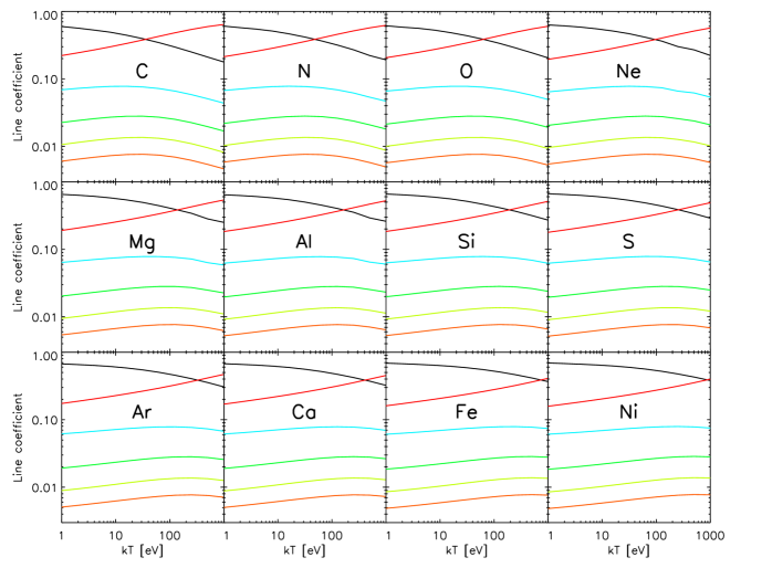
Figure 2: Line coefficients for the brightest features resulting from radiative recombination forming H-like ions. Ly $\alpha$ (black), Ly $\beta$ (cyan), Ly $\gamma$ (green), Ly $\delta$ (olive), and Ly $\epsilon$ (orange) are shown, along with the ground-state RRC (red). Division of the observed line luminosity by the line coefficient gives the radiative recombination rate $\Delta_{z-1}^{z}$ (at an assumed temperature). Division of $\Delta_{z-1}^{z}$ by $C_{\mathrm{total}}$ in Fig. 4 gives the ionic emission measure EM${}_{z-1}=\int n_{\mathrm{z-1,g}}n_{\mathrm{e}}dV$ (see Eq. 19).

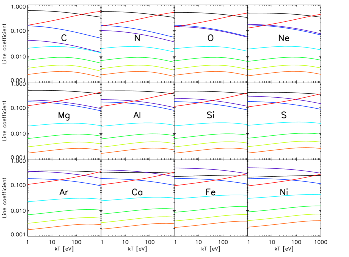
Figure 3: Line coefficients for the brightest features resulting from pure radiative recombination forming He-like ions in a low density plasma. Forbidden (black), intercombination (purple), resonance (blue), He$\beta$ (cyan), He$\gamma$ (green), He$\delta$ (olive), and He$\epsilon$ (orange) are shown as well as the ground-state RRC (red). Division of the observed line luminosity by the line coefficient gives the radiative recombination rate $\Delta_{z-1}^{z}$. Division of $\Delta_{z-1}^{z}$ by $C_{\mathrm{total}}$ in Fig. 5 gives the ionic emission measure EM${}_{z-1}=\int n_{\mathrm{z-1,g}}n_{\mathrm{e}}dV$ (see Eq. 19). Caveat: At the low temperature end, only radiative recombination is important, but at the high temperature end ($kT\sim E_{0}$ where $E_{0}$ is the resonance line energy), additional contributions to the line emission (not included) from dielectronic recombination and collisional excitation become important. Also, high densities or strong ambient UV fields can convert $f\rightarrow i$, as explained in §4.4.

In Figs. 2 and 3, we plot the line coefficients for the principal lines of H-like and He-like ions, respectively. Also shown in Figs. 4 and 5 are the corresponding $C_{\mathrm{total}}$ as a function of temperature. Together, these plots allow for the determination of the total recombination rates as well as ionic emission measures for a given photoionized plasma spectrum. In addition, we provide the standard He-like triplet ratios $R=f/i$ and $G=(i+f)/r$ (Gabriel & Jordan 1969) for pure radiative recombination as a function of temperature in Fig. 6. We stress that since the He-like curves do not include the additional contributions from dielectronic recombination and collisional excitation present at the high temperature end, direct comparison with data for these high temperatures should be avoided. Explanation of exactly how these calculations were carried out is provided below in §4.6.

We again stress the neglect of the well-observed process of forbidden-to-intercombination line conversion in the He-like triplets through excitation of the long-lived 2 ³S₁ level up to the 2 ³P multiplet (Gabriel & Jordan 1969). Though we do not take this into account here (and it is not included in PHOTOION), it is simple enough to determine the effects on the He-like triplet ratio $R=f/i$ of electron collisional excitation which is dependent on $n_{\mathrm{e}}$ and $T_{\mathrm{e}}$ (e.g., Porquet & Dubau 2000) and/or of UV photoexcitation which is dependent only on $F(E_{0})$ (e.g., Kahn et al. 2001).

4.5 Radiation-Driven Emission from Other Ions

Li-like and lower-ionization-state ions are in general more complicated for a number of reasons. Excitations and ionizations can now lead to excited levels capable of autoionization of single and, importantly, multiple electrons. This implies that the strict equivalence between the single-electron removal rate (either through photoionization or single-electron autoioinization following photoexcitation) and the recombination rate between neighboring charge states are no longer necessarily equal. However, autoionizations removing more than one electron are typically negligible compared to photoionizations and single-electron autoionization (though this statement deserves further investigation). Therefore, this equivalence is likely still a very good approximation, and can be expressed as follows:

$$\Delta_{z-1}^{z}=\int n_{z-1,g}n_{\mathrm{e}}C_{\mathrm{total}}\ dV=\int n_{z,g}\bigg{(}\sum_{j}R_{z,g}^{z-1,j}+\sum_{j}R_{z,g}^{z,j}f^{D}_{z,j}\bigg{)}dV,$$ (22)

where $C_{\mathrm{total}}$ is the total recombination rate coefficient (now for both radiative and dielectronic recombination) and $f^{D}_{z,j}$ denotes the fraction of decays from $z,j$ that lead to electron removal via autoionization (hence the $D$ superscript).

We now focus on Eq. 11, which describes the line emission. As a further approximation, we drop the last term on the RHS of Eq. 11, which gives all autoionizations from lower charge states landing on the excited level $z,i$. This allows us to consider transitions only within the same ion. As for Eq. 17, we assume that the temperature range is small enough so that $C_{z-1,g}^{z,i}/C_{\mathrm{total}}$ is independent of temperature. Then, from Eqs. 11 and 22, we obtain:

$$N_{z,i}\bigg{(}\sum_{j<i}A_{z,i}^{z,j}+\sum_{1\leq k<z}\sum_{j}D_{z,i}^{z-k,j}\bigg{)}-\sum_{j>i}N_{z,j}A_{z,j}^{z,i}\approx\frac{C_{z-1,g}^{z,i}}{C_{\mathrm{total}}}\int n_{z,g}\bigg{(}\sum_{j}R_{z,g}^{z-1,j}+\sum_{j}R_{z,g}^{z,j}f^{D}_{z,j}\bigg{)}dV$$

$$+\int n_{z,g}R_{z,g}^{z,i}dV+\int n_{z+1,g}R_{z+1,g}^{z,i}dV.$$ (23)

The linearity of Eq. 23 allows us to separate out the respective contributions to all $N_{z,i}$ from photoionization/autoionization (eventually producing recombinations, both radiative and dielectronic) and the fraction of photoexcitations that produce radiative decays: $N_{z,i}=N^{\mathrm{REC}}_{z,i}+N^{\mathrm{DEC}}_{z,i}$. For photoionization/autoionization which produce eventual recombinations, we have:

$$N^{\mathrm{REC}}_{z,i}\sum_{j<i}A_{z,i}^{z,j}-\sum_{j>i}N^{\mathrm{REC}}_{z,j}A_{z,j}^{z,i}\approx\frac{C_{z-1,g}^{z,i}}{C_{\mathrm{total}}}\int n_{z,g}\bigg{(}\sum_{j}R_{z,g}^{z-1,j}+\sum_{j}R_{z,g}^{z,j}f^{D}_{z,j}\bigg{)}dV.$$ (24)

We have neglected the $\sum_{1\leq k<z}\sum_{j}D_{z,i}^{z-k,j}$ terms, which for the low temperatures typical of photoionized plasmas do not usually contribute significantly to the recombination spectra. These terms are retained, however, in Eq. 25, where they are essential for excitations and ionizations resulting in levels capable of autoionization. The system of equations represented by Eq. 24 can be thought of as the exact solution of the line spectrum for a given recombination rate onto each level $i$ of $\Delta_{z-1}^{z}C_{z-1,g}^{z,i}/C_{\mathrm{total}}$, where $\Delta_{z-1}^{z}$ is the total recombination rate. Similarly, for photoexcitation, we obtain

$$N^{\mathrm{DEC}}_{z,i}\bigg{(}\sum_{j<i}A_{z,i}^{z,j}+\sum_{1\leq k<z}\sum_{j}D_{z,i}^{z-k,j}\bigg{)}-\sum_{j>i}N^{\mathrm{DEC}}_{z,j}A_{z,j}^{z,i}\approx\int n_{z,g}R_{z,g}^{z,i}dV+\int n_{z+1,g}R_{z+1,g}^{z,i}dV.$$ (25)

Here, for the first time on the LHS, we must integrate over both $n_{z,g}$ and $n_{z+1,g}$, the latter represent all photoionizations that leave the ion in an excited level (for photoionization of H- and He-like ions, this is always the ground state). As a further simplification to Eq. 25, we can discard the last term on the LHS, which describes feeding of $z,i$ by all higher excitation levels:

$$N^{\mathrm{DEC}}_{z,i}\bigg{(}\sum_{j<i}A_{z,i}^{z,j}+\sum_{1\leq k<z}\sum_{j}D_{z,i}^{z-k,j}\bigg{)}\approx\int n_{z,g}R_{z,g}^{z,i}dV+\int n_{z+1,g}R_{z+1,g}^{z,i}dV.$$ (26)

This directly gives the fluorescence yield for each excited level without having to perform a matrix inversion.

4.6 Atomic Data Calculation and Implementation

In the foregoing, we have delineated how a series of approximations can reduce solution of the spectrum of each ion to a seemingly simple matrix inversion. We now discuss how these matrix inversions are currently implemented in PHOTOION.

Throughout, we use atomic data generated by the atomic code FAC (Gu 2002; Gu 2003). For recombination calculations onto all relevant ions (for which recombination produces X-ray features), we explicitly calculate all levels up to principal quantum number $n\leq 25$ and all E1, E2, M1, and M2 transitions $n^{\prime}l^{\prime}\rightarrow nl$ with $n,n^{\prime}\leq 25$. Explicit calculation of all levels for $n=45$ allows for interpolation for levels $n=26$–44. Using the H-like approximation for the recombination cross-sections, we sum all recombinations onto levels $n>45$ and then spread this contribution over $n=45$. Solution of the relevant matrices (such as in Eqs. 17 and 18) can now be obtained using only levels with $n\leq 45$. We also include all important two-photon decays for both H-like and He-like (Drake 1986); such decays are not calculated by FAC. Similar calculations were carried out to determine the contribution from radiative and dielectronic recombination forming L-shell ions for all ions of interest in the X-ray regime. Due to the large number of excited levels for L-shell ions, inversions of the relevant matrix (represented by Eq. 24) required further approximations described in Gu (2002) and Gu (2003).

Photoexcitation to all $n\leq 25$ levels ($n\leq 100$ for H- and He-like ions) is calculated directly from the atomic code results for the oscillator strengths $f_{ji}$ and radiative decay rates $A_{ji}$ using the standard Voigt profile for line absorption/emission discussed in §4.1. (Caveat: Since we do not presently calculate photoexcitation to higher $n$ levels — ideally out to $n\rightarrow\infty$ — there is an artificial discontinuity at the photoelectric edges.) For radiative decay following valence-shell photoexcitation, solving the matrix for all excited levels is unnecessary since the dominant decay is the direct decay back to the ground state. Currently, to simplify and speed up the code, we therefore assume that every photoexcitation always produces a transition back to the ground state (even for photoexcitations to levels capable of autoionization, see below). This approximation is reliable for all important valence-shell transitions at the few percent level for reemission in an optically thin medium. For the same reason, we also only use the radiative decay rate to the ground for parameter $x$ in the Voigt function (Eq. 9). Velocity widths in many X-ray absorbers have recently been observed to be significantly larger than the expected thermal width, which itself is much larger than the natural line width, making this a safe approximation.

To increase the accuracy for especially important transitions (currently only in the H- and He-like ions), we verified and, if necessary, modified important photoelectric cross sections, oscillator strengths, and especially wavelengths with previously-published calculations and experimental results from Verner et al. (1996); Verner, Verner, & Ferland (1996); and NIST .

Also, not yet included is the calculation of all possible autoionization rates following photoexcitation or photoionization to determine total resulting line fluorescence. Currently, all photoexcitations are assumed to decay directly back to the ground state, leading to a sometimes gross overprediction of fluorescence for some excited levels with especially high autoionization rates. Oppositely, fluorescence resulting from photoionization is currently absent in the code. Prospects for inclusion of these rates are discussed in §7.

5 Irradiated Cone Model

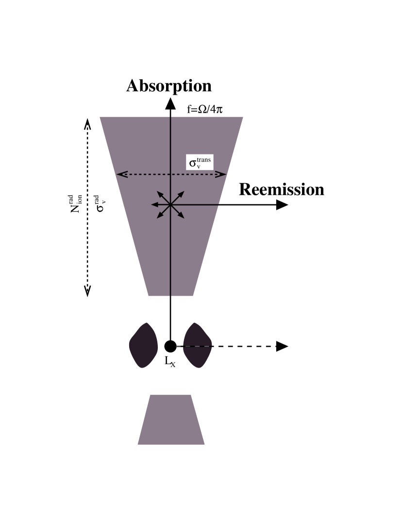
Figure 7: Simple cartoon of irradiated cone model (not to scale). The central nuclear component which irradiates the cone is shown as the black spot. The labels “Absorption” or “Reemission” denote the two main orientations of interest. The following model parameters are indicated: $f=\Omega/4\pi$ (covering factor), $N^{\mathrm{rad}}_{\mathrm{ion}}$ (each individual ionic column density), $\sigma_{v}^{\mathrm{rad}}$ (radial gaussian velocity width), $\sigma_{v}^{\mathrm{trans}}$ (transverse gaussian velocity width), and $L_{X}$ (irradiating spectrum). In the “Absorption” direction, in addition to features imprinted by line and edge absorption, reemission in the cone may also provide an additional contribution (see Fig. 8). Also, in the “Reemission” direction, the intrinsic continuum may or may not be obscured by an additional medium (see Fig. 9). Finally, we note that some sources may also exhibit a second cone (shown at the bottom of the figure).

In order to integrate the expressions on the right-hand sides of Eqs. 17 and 23, we must first introduce our model. The simplest version consists of an isotropic cone irradiated by a nuclear source with photon luminosity spectrum $L(E)=AE^{-\Gamma}$ (e.g., in units photons s^-1 keV^-1). We characterize the cone by a solid angle $\Omega$, radial column density $G$, and radial gaussian velocity distribution $\sigma_{v}^{\mathrm{rad}}$ (which broadens all radiative cross-sections) for the ground state of each particular ion (Fig. 7). We first consider the more general non-isotropic case: $L(E,\vec{\theta})$, $G(\vec{\theta})$, and $\sigma_{v}^{\mathrm{rad}}(\vec{\theta})$, where $\vec{\theta}\equiv(\theta,\phi)$.

Employing the above assumptions, we obtain for the $R$ coefficients pertaining to a particular ion $n_{z,i}$ (with $z^{\prime}=z$ for photoexcitation and $z^{\prime}=z-1$ for photoionization):

$$R_{z,i}^{z^{\prime},j}(F(E,r,\vec{\theta}))=\int\big{[}\sigma^{R}\big{]}_{z,i}^{z^{\prime},j}(E,\vec{\theta})\bigg{(}\frac{L(E,\vec{\theta})}{4\pi r^{2}}e^{-\tau(E,r,\vec{\theta})}\bigg{)}dE,$$ (27)

where $\tau(E,r,\vec{\theta})=\int_{0}^{r}\sum_{\{Z,z\}}{n_{Z,z,g}}(r^{\prime},\vec{\theta})\sigma^{R}_{Z,z}(E,\vec{\theta})dr^{\prime}$ and $\sigma^{R}_{Z,z}(E,\vec{\theta})$ denotes the total radiative cross section for all radiation-driven transitions from the ground state of a particular element $A$ with $z$ electrons, with all cross sections already implicitly convolved with a possibly angular-dependent velocity distribution along the cone, $\sigma^{\mathrm{rad}}_{v}(\vec{\theta})$. $L(E,\vec{\theta})$ is the intrinsic nuclear luminosity (again with possible angular dependence). The exponential takes into account absorption along the cone due to the ground-state number densities $n_{z,g}$.

We now integrate the $R$ coefficients times the appropriate ionic density over volume to get the total photoexcitation (or photoionization) rate in the plasma:

$$\int n_{z,g}(r,\vec{\theta})R_{z,g}^{z^{\prime},j}(F(E,r,\vec{\theta}))dV=\int dE\int\frac{d\Omega}{4\pi}\int dr\ n_{z,g}(r,\vec{\theta})\big{[}\sigma^{R}\big{]}_{z,g}^{z^{\prime},j}(E,\vec{\theta})\ L(E,\vec{\theta})e^{-\tau(E,r,\vec{\theta})}.$$ (28)

There are two different assumptions which can be made at this point to simplify this integral. The first assumption is that only the particular ion of interest contributes to the opacity. This is fairly robust if column densities of all other ions are low enough that only discrete line absorption is present in the spectrum, since the opacity due to lines alone is usually negligible. Under this assumption, the opacity $\tau$ is only dependent on the particular ion of interest; therefore, $d\tau\equiv d\tau(E,r,\vec{\theta})=n_{z,g}(r,\vec{\theta})\sigma^{R}_{z}(E,\vec{\theta})dr$, and we can rewrite Eq. 28 as:

$$\int n_{z,g}(r,\vec{\theta})R_{z,g}^{z^{\prime},j}(F(E,r,\vec{\theta}))dV=\int dE\int\frac{d\Omega}{4\pi}\int_{0}^{\tau}d\tau^{\prime}\ L(E,\vec{\theta})e^{-\tau^{\prime}}.$$ (29)

Upon integration over $\tau^{\prime}$, this simplifies to:

$$\int n_{z,g}R_{z,g}^{z^{\prime},j}dV=\int\frac{d\Omega}{4\pi}G_{z}(\vec{\theta})\int dE\ \big{[}\sigma^{R}\big{]}_{z,g}^{z^{\prime},j}(E,\vec{\theta})\ L(E,\vec{\theta})\frac{1-e^{-\tau(E,\vec{\theta})}}{\tau(E,\vec{\theta})},$$ (30)

where $G_{z}$ is the ground-state column density for ions (with $z$ electrons) of the particular element under consideration.

Alternatively, a second possible assumption could be that relative ionic abundances are independent of radius. Starting once again from Eq. 28, we now simply multiply and divide by the sum in large parentheses in the following expression:

$$\int n_{z,g}(r,\vec{\theta})R_{z,g}^{z^{\prime},j}(F(E,r,\vec{\theta}))dV=\int dE\int\frac{d\Omega}{4\pi}\int dr\ \frac{n_{z,g}(r,\vec{\theta})\big{[}\sigma^{R}\big{]}_{z,g}^{z^{\prime},j}(E,\vec{\theta})}{\sum_{\{Z^{\prime},z\}}{n_{Z^{\prime},z,g}}(r,\vec{\theta})\sigma^{R}_{Z^{\prime},z}(E,\vec{\theta})}\bigg{(}\sum_{\{Z^{\prime},z\}}n_{Z^{\prime},z,g}(r,\vec{\theta})\sigma^{R}_{Z^{\prime},z}(E,\vec{\theta})\bigg{)}\ L(E,\vec{\theta})e^{-\tau(E,r,\vec{\theta})}.$$ (31)

Recall that $d\tau(E,r,\vec{\theta})=\sum_{\{Z,z\}}{n_{Z,z,g}}(r,\vec{\theta})\sigma^{R}_{Z,z}(E,\vec{\theta})dr$. Therefore, the sum in large parentheses in Eq. 31 times $dr$ is just $d\tau$. Therefore, by our central assumption that all relative ionic abundances are independent of $r$, the fractional term in Eq. 31 is also independent of $r$ and can be replaced by a fraction involving only the total integrated ionic column densities $G_{Z,z}$:

$$\int n_{z,g}(r,\vec{\theta})R_{z,g}^{z^{\prime},j}(F(E,r,\vec{\theta}))dV=\int\frac{d\Omega}{4\pi}\int dE\frac{G_{z}(\vec{\theta})\big{[}\sigma^{R}\big{]}_{z,g}^{z^{\prime},j}(E,\vec{\theta})}{\sum_{\{Z,z\}}{G_{Z,z}}(\vec{\theta})\sigma^{R}_{Z,z}(E,\vec{\theta})}\ L(E,\vec{\theta})\int_{0}^{\tau}e^{-\tau^{\prime}}d\tau^{\prime}.$$ (32)

Upon integration over $\tau$, we obtain:

$$\int n_{z,g}R_{z,g}^{z^{\prime},j}dV=\int\frac{d\Omega}{4\pi}G_{z}(\vec{\theta})\int dE\ \big{[}\sigma^{R}\big{]}_{z,g}^{z^{\prime},j}(E,\vec{\theta})\ L(E,\vec{\theta})\frac{1-e^{-\tau(E,\vec{\theta})}}{\tau(E,\vec{\theta})},$$ (33)

which, interestingly, is identical to Eq. 30.

For the simplest model of an isotropic cone of material with solid angle extent $\Omega$ characterized by angle-independent radial column density $G$, radial gaussian velocity distribution $\sigma_{v}$, and nuclear photon luminosity spectrum $L(E)$, the identical expressions derived above (Eqs. 30 and 33) reduce to:

$$\int n_{z,g}R_{z,g}^{z^{\prime},j}dV=\frac{\Omega}{4\pi}G_{z}\int dE\ \big{[}\sigma^{R}\big{]}_{z,g}^{z^{\prime},j}(E)\ L(E)\frac{1-e^{-\tau(E)}}{\tau(E)}.$$ (34)

This equation serves as the basis of PHOTOION.

6 Spectra for Various Absorption and Reemission Geometries Calculated with PHOTOION

The XSPEC model PHOTOION allows the calculation of spectra arising from different absorption and reemission geometries. Below, we provide examples of some simple geometries possible with PHOTOION.

6.1 Absorption

An example of a spectrum due to pure absorption is given in Fig. 8a. The imprinting of absorption features on the intrinsic continuum is determined by $e^{-\tau(E)}$ with

$$\tau(E)\equiv\tau(E,\vec{\theta})=\int_{0}^{r}\sum_{\{Z,z\}}{n_{Z,z,g}}(r^{\prime},\vec{\theta})\sigma^{R}_{Z,z}(E,\vec{\theta})dr^{\prime}=\sum_{\{Z,z\}}\int_{0}^{r}{n_{Z,z,g}}(r^{\prime},\vec{\theta})\sigma^{R}_{Z,z}(E,\vec{\theta})dr^{\prime}=\sum_{\{Z,z\}}G_{Z,z}\sigma^{R}_{Z,z}(E,\vec{\theta}).$$ (35)

Here, $\sigma^{R}_{Z,z}(E,\vec{\theta})$ denotes the total radiative cross section (in the line-of-sight direction $\vec{\theta}$) for all radiation-driven transitions from the ground state of each ion, with all cross-sections implicitly convolved with the velocity distribution characterized by width $\sigma_{v}^{\mathrm{rad}}$. This model can also be calculated using the related multiplicative XSPEC model MPABS (multi-phase absorber), which allows for pure absorption studies through the independent variation of each ionic column density. These models should be useful in particular for understanding the complex, multi-phase absorption observed in a number of Seyfert 1 galaxy spectra (e.g., Kaastra et al. 2000, Sako et al. 2001, Behar, Sako, & Kahn 2001).

6.2 Reemission

Observations transverse to the cone yield line spectra resulting from reemission in the cone. We concentrate on the dominant reemission from H- and He-like ions for simplicity (the contributions due to lower-charge-state ions is straightforward to include). The final spectrum of transitions to the ground state of all relevant K-shell ions is then simply the sum of all ionic contributions:

$$\mathrm{Reemission}(E)=\sum_{j,i}N_{z,j}A_{z,j}^{z,i}l_{j\rightarrow i}(E)+\Delta_{z-1}^{z}\frac{C_{z-1,g}^{z,g}}{C_{\mathrm{total}}}r(E),$$ (36)

where $\Delta_{z-1}^{z}$ is the total recombination rate calculated from Eq. 13 and $l_{j\rightarrow i}(E)$ is the appropriate Voigt line profile (normalized to 1) using velocity distribution $\sigma_{v}^{\mathrm{trans}}$ and $r(E)$ is the ground-state recombination profile (normalized to 1) convolved with $\sigma_{v}^{\mathrm{trans}}$. In general, $\sigma_{v}^{\mathrm{trans}}$ may not necessarily be equal to $\sigma_{v}^{\mathrm{rad}}$. Explicitly, and without velocity convolution, the recombination profile is simply:

$$r(E)\propto f(E-E_{\mathrm{th}};kT_{\mathrm{e}})\frac{E^{2}}{\sqrt{E-E_{\mathrm{th}}}}\sigma_{\mathrm{PI}}(E),$$ (37)

where $f(E-E_{\mathrm{th}};kT_{\mathrm{e}})$ is the Maxwellian distribution, evaluated at $E-E_{\mathrm{th}}$ and specified by temperature $kT_{\mathrm{e}}$, and $\sigma_{\mathrm{PI}}(E)$ is the photoionization cross section, with $\sigma_{\mathrm{PI}}(E)=0$ for $E<E_{\mathrm{th}}$. The contribution from radiative and dielectronic recombination forming lower-ionization-state ions is also straightforward to include. Examples of reemission spectra for differing amounts of obscuration towards the intrinsic continuum are shown in Fig. 9).

If the emission regions are moderately optically thick to their emission, then the reemitted spectra will be modified. Higher-order transitions ($n\rightarrow 1$ with $n>2$) will be degraded through multiple scattering to lower-order transitions (at sufficiently high optical depths, all higher order lines are converted to $n=2\rightarrow 1$ transitions). This reprocessing can provide an estimate of the overall optical thickness of the medium. In Fig. 13 of Kinkhabwala et al. (2002), the diagnostic value of this effect in H-like and He-like line series is illustrated. The lines shown in that plot give the column density and velocity width in (assuming a roughly spherical medium) corresponding to 10% conversion of the Ly$\beta$ photons to Ly$\alpha$ and, similarly, 10% conversion of He$\beta$ to He$\alpha$ transitions for C through Mg (degradation percentage can be scaled arbitrarily in these plots).

6.3 Absorption Plus Reemission

Even if the ionization cone is viewed in absorption, there is some amount of the reprocessed emission which will be reemitted in the observer’s direction (see Fig. 7). The total spectrum can be written as $\mathrm{Spectrum}(E)=L(E)\mathrm{e}^{-\tau(E)}+\mathrm{Reemission}(E)$, where $\mathrm{Reemission}(E)=\mathrm{Decay}(E)+\mathrm{Recombination}(E)$, with $\mathrm{Decay}(E)$ giving the total contribution from radiative decay following photoexcitation and $\mathrm{Recombination}(E)$ giving the total contribution of both radiative and dielectronic recombination. Both $\mathrm{Decay}(E)$ and $\mathrm{Reemission}(E)$ implicitly contain the details of absorption in the cone, as shown below.

In order to account for absorption of the reemitted spectrum in the cone we must make some further assumptions. First, we assume that the cone is sufficiently narrow so that the absorption factor pertaining to any region of the cone is just dependent on radius. We define two such absorption factors: $\tau_{o}(E,r)=\int_{r_{o}}^{r}\sum_{\{Z,z\}}n_{Z,z,g}(r)\big{[}\sigma^{R}\big{]}_{Z,z,g}(E)$, representing absorption from the inner radius $r_{o}$ of the cone to $r$, and $\tau_{f}(E,r)=\int_{r}^{r_{f}}\sum_{\{Z,z\}}n_{Z,z,g}(r)\big{[}\sigma^{R}\big{]}_{Z,z,g}(E)$, representing absorption from $r$ to the outer radius of the cone $r_{f}$. Clearly, the total opacity is just $\tau(E)=\tau_{o}(E,r)+\tau_{f}(E,r)$ for any value of $r$.

First, we derive a general expression for $\mathrm{Decay}(E)$. For simplicity, we assume that photoexcitation corresponds to coherent resonant scattering (in contrast to statements made in §2). The relevant spectrum expressed as a simple integral over the cone can then be written as:

$$\mathrm{Decay}(E) = \sum_{\{Z,z\}}\int F(E,r)n_{Z,z,g}(r)\sum_{j}\big{[}\sigma^{R}\big{]}_{Z,z,g}^{Z,z,j}(E)\mathrm{e}^{-{\tau_{f}(r)}}r^{2}drd\Omega=$$ (38)

$$\sum_{\{Z,z\}}\int\frac{L(E)\mathrm{e}^{-\tau_{0}(r,E)}}{4\pi r^{2}}n_{Z,z,g}(r)\sum_{j}\big{[}\sigma^{R}\big{]}_{Z,z,g}^{Z,z,j}(E)\mathrm{e}^{-{\tau_{f}(r,E)}}r^{2}drd\Omega=$$

$$\frac{\Omega}{4\pi}L(E)\mathrm{e}^{-\tau(E)}\sum_{\{Z,z\}}\sum_{j}\big{[}\sigma^{R}\big{]}_{Z,z,g}^{Z,z,j}(E)\int n_{Z,z,g}(r)dr=$$

$$\frac{\Omega}{4\pi}L(E)\mathrm{e}^{-\tau(E)}\sum_{\{Z,z\}}\sum_{j}G_{Z,z}\big{[}\sigma^{R}\big{]}_{Z,z,g}^{Z,z,j}(E).$$

Accounting for absorption of the reemission contribution from recombination is more difficult due to the need to integrate over each photoelectric edge to determine the photoionization (and, therefore, recombination) rate. Here, we define $R_{Z,z}(E)$ to be the spectrum (properly normalized) of recombination (radiative and dielectronic) forming ion $Z,z$. Total recombinations are balanced with photoionizations (resulting either from direct photoionization or indirect ionization via autoionization following photoexcitation; though only the contribution from the former is shown below for simplicity). This yields:

$$\mathrm{Recombination}(E) = \sum_{\{Z,z\}}R_{Z,z}(E)\int\bigg{(}\int F(E^{\prime},r)n_{Z,z,g}(r)\sum_{j}\big{[}\sigma^{R}\big{]}_{Z,z,g}^{Z,z-1,j}(E^{\prime})dE^{\prime}\bigg{)}\mathrm{e}^{-{\tau_{f}(r)}}r^{2}drd\Omega=$$ (39)

$$\frac{\Omega}{4\pi}\sum_{\{Z,z\}}R_{Z,z}(E)\int\bigg{(}\int L(E^{\prime})\mathrm{e}^{-\tau_{0}(r,E^{\prime})}\sum_{j}\big{[}\sigma^{R}\big{]}_{Z,z,g}^{Z,z-1,j}(E^{\prime})dE^{\prime}\bigg{)}\mathrm{e}^{-{\tau_{f}(r)}}n_{Z,z,g}(r)dr.$$

Here, the integral over energy in parentheses is still a function of $r$ through $\tau_{o}(r,E)$, requiring a costly double integral. In order to speed up this calculation, we would like to split this double integral into two sequential integrations over $E$ and then $r$. This requires approximating the opacity term within the energy integral as some average opacity independent of radius, $\mathrm{e}^{-\tau_{o}(r,E)}\approx\mathrm{Opacity}(E)$. Employing once again the assumption that all ionic ratios are constant throughout the cone, we obtain:

$$\mathrm{Recombination}(E)=\frac{\Omega}{4\pi}\sum_{\{Z,z\}}R_{Z,z}(E)\bigg{(}\int L(E^{\prime})\mathrm{Opacity}(E^{\prime})\sum_{j}\big{[}\sigma^{R}\big{]}_{Z,z,g}^{Z,z-1,j}(E^{\prime})dE^{\prime}\bigg{)}\times$$ (40)

$$\int\mathrm{e}^{-{\tau_{f}(r,E)}}\frac{n_{Z,z,g}(r)}{\sum_{\{Z^{\prime},z\}}{n_{Z^{\prime},z,g}(r)\sigma^{R}_{Z^{\prime},z}(E)}}\sum_{\{Z^{\prime},z\}}n_{Z^{\prime},z,g}(r)\sigma^{R}_{Z^{\prime},z}(E)dr$$ (41)

Recalling that $d\tau_{f}(r,E)=-\sum_{\{Z^{\prime},z\}}n_{Z^{\prime},z,g}(r)\sigma^{R}_{Z^{\prime},z}(E)dr$, we can integrate this expression (e.g., see Eqs. 31–33), obtaining:

$$\mathrm{Recombination}(E)=\frac{\Omega}{4\pi}\sum_{\{Z,z\}}G_{Z,z}R_{Z,z}(E)\frac{1-\mathrm{e}^{-\tau(E)}}{\tau(E)}\int L(E^{\prime})\mathrm{Opacity}(E^{\prime})\sum_{j}\big{[}\sigma^{R}\big{]}_{Z,z,g}^{Z,z-1,j}(E^{\prime})dE^{\prime}.$$ (42)

Useful lower and upper limits to the recombination contribution are obtained by taking $\mathrm{Opacity}(E)=\mathrm{e}^{-\tau(E)}$ and $\mathrm{Opacity}(E)=1$, respectively. Spectra resulting from assumption of either limit can be calculated with PHOTOION (see Fig. 8).

7 Discussion

The models presented in this paper have already received experimental verification through X-ray spectra of multiple accretion-powered astrophysical sources. In particular, application of our model to the remarkable XMM-Newton spectrum of the brightest, prototypical Seyfert 2 galaxy, NGC 1068 (Kinkhabwala et al. 2002), provided the first quantitative test of a photoionization code (e.g., the gratifying confirmation of the ratio of intercombination line to RRC in O VII). In addition, the self-consistent inclusion of photoexcitation and resulting radiative decay allowed for discrimination between emission mechanisms in the spectrum of NGC 1068, providing a robust upper limit to any additional contribution from hot plasmas. Observations of NGC 1068 also provided the motivation for the seemingly ad hoc assumption taken in §5 that all ionic ratios are constant throughout the cone (Brinkman et al. 2002; Ogle et al. 2003), as was explained in §1. We expect that PHOTOION (and associated codes PHSI, MPABS, and SIABS) will continue to be of use in the description of astrophysical photoionized plasmas existing in a variety of sources, including AGN, X-ray binaries, cataclysmic variables, stellar winds of early-type stars, GRB afterglows, and the IGM.

Lastly, as mentioned in §4.6, radiative and autoionizing decay rates (as well as the resulting fluorescence intensities) for levels capable of autoionization have not yet been properly included. Especially important are the Fe K-shell transitions in Fe M-shell and L-shell ions. The number of atomic levels involved in these calculations is large, but not prohibitive. These represent the final atomic calculations necessary to “complete” PHOTOION, at least in terms of the assumptions taken in this paper. These rates should eventually be included in a future version of the code.

Figure 1: Highly-simplified grotrian diagrams depicting all of the relevant atomic processes for photoionized plasmas. The top two diagrams depict photoexcitation and its inverse process of radiative decay (only the dominant direct decay path is shown, but other decay paths are possible). The next two diagrams depict photoionization and the inverse process of radiative recombination and radiative cascade. Another important inverse process to photoionization (especially for multi-electron ions) is the two-step process of dielectronic recombination, depicted in the next two diagrams. The last three diagrams depict photoexcitation up to a level capable of autoionization followed by either radiative decay or autoionization; these diagrams can be trivially modified to describe photoionization to levels capable of autoionization as well.

      

        

Figure 4: The temperature dependence of $C_{\mathrm{total}}$ for radiative recombination forming H-like ions (see also Fig. 2).

Figure 5: The temperature dependence of $C_{\mathrm{total}}$ for radiative recombination forming He-like ions (see also Fig. 3). Dielectronic recombination, which becomes important at the high temperature end ($kT\sim E_{0}$ where $E_{0}$ is the resonance line energy), has not been included.

      

Figure 6: He-like triplet ratios $R=f/i$ and $G=(i+f)/r$ for pure radiative recombination for elements C, N, O, Ne, Mg, Al, Si, S, Ar, Ca, Fe, and Ni (from top to bottom). At the low temperature end, only radiative recombination is important, but at higher temperatures ($kT\sim E_{0}$ where $E_{0}$ is the resonance line energy), additional contributions (not included) from dielectronic recombination and collisional excitation become important.

                     

            

Figure 8: Three examples of multi-phase “Absorption” spectra (see Fig. 7) calculated by PHOTOION: a) Pure absorption, b) Absorption plus reemission (upper limit assuming $\mathrm{Opacity}(E)=1$, see §6.3), and c) Absorption plus reemission (lower limit assuming $\mathrm{Opacity}(E)=\mathrm{e}^{-\tau(E)}$, see §6.3). For all spectra, we take $\sigma_{v}^{\mathrm{rad}}=400$ km s^-1 and a power-law slope of $\Gamma=1.8$. And, for spectra in panels b) and c), we further assume a covering fraction of $f=\Omega/4\pi=0.15$ for the reemission component.

            

Figure 9: “Reemission” analogue (see Fig. 7) to the same absorption model used in the top panel of Fig. 8. For all spectra, we take $\sigma_{v}^{\mathrm{rad}}=\sigma_{v}^{\mathrm{trans}}=400$ km s^-1, $\Gamma=1.8$, and $f=\Omega/4\pi=0.15$. Here the three panels correspond to differing amounts of obscuration along the observer’s line-of-sight to the intrinsic continuum: a) Pure reemission spectrum (intrinsic continuum is completely absorbed), b) Reemission spectrum plus moderately-absorbed intrinsic continuum (with neutral opacity towards intrinsic continuum equivalent to $N_{\mathrm{H}}=5.0\,$e22 cm^-2), and c) Reemission plus unabsorbed intrinsic continuum.

References

- Arnaud (1996) Arnaud, K.A. 1996, in ASP Conf. Ser. 101, Astronomical Data Analysis Software Systems V, ed. G.H. Jacoby & J. Barnes (San Francisco: ASP), 17
- Behar, Sako, & Kahn (2001) Behar, E., Sako, M., & Kahn, S.M. 2001, ApJ, 563, 497
- Brinkman et al. (2002) Brinkman, A.C., Kaastra, J.S., van der Meer, R.L.J., Kinkhabwala, A., Behar, E., Kahn, S.M., Paerels, F.B.S., &, Sako, M. 2002, A&A, 396, 761
- Cottam et al. (2001) Cottam, J., Kahn, S.M., Brinkman, A.C., den Herder, J.W., & Erd, C. 2001, A&A, 365, L277
- Drake (1986) Drake, G.W.F. 1986, PRA, 34, 2871
- Dumm et al. (2002) Dumm, T., Güdel, M., Schmutz, W., Audard, M., Schild, H., Leutenegger, M., & van der Hucht, K. 2002, in ”New Visions of the X-ray Universe in the XMM-Newton and Chandra Era”, ed. F. Jansen, in press (available at http://www.astro.columbia.edu/ audard/publ/newvisions/tdumm-b1.ps)
- den Herder et al. (2001) den Herder, J.W., et al. 2001, A&A, 365, L7
- Einstein (1917) Einstein, A. 1917, Phys. Z., 18, 121
- Jansen et al. (2001) Jansen, F. et al. 2001, A&A, 365, L1
- Gabriel & Jordan (1969) Gabriel, A.H., & Jordan, C. 1969, MNRAS, 145, 241
- Gu (2002) Gu, M.F. 2002, ApJ, 579, L103
- Gu (2003) Gu, M.F. 2003, ApJ, 582, 1241
- Halpern & Grindlay (1980) Halpern, J.P., & Grindlay, J.E. 1980, ApJ, 242, 1041
- Kaastra (1992) Kaastra, J.S. 1992, An X-Ray Spectral Code for Optically Thin Plasmas, Internal SRON-Leiden REport, updated version 2.0
- Kaastra et al. (2000) Kaastra, J.S., Mewe, R., Liedahl, D.A., Komossa, S., & Brinkman, A.C. 2000, A&A, 354, L83
- Kahn et al. (2001) Kahn, S.M., Leutenegger, M.A., Cottam, J., Rauw, G., Vreux, J.-M., den Boggende, A.J.F., Mewe, R. & Güdel, M. 2001, A&A, 365, L312
- Kallman et al. (1996) Kallman, T.R., Liedahl, D., Osterheld, A., Goldstein, W., & Kahn, S. 1996, ApJ, 465, 994
- Kallman & McCray (1982) Kallman, T.R., & McCray, R. 1982, APJS, 50, 263
- Kinkhabwala et al. (2002) Kinkhabwala, A., et al. 2002, ApJ, 575, 732
- Krolik, McKee, & Tarter (1981) Krolik, J.H., McKee, C.F., & Tarter, C.B. 1981, ApJ, 249, 422
- Liedahl (1999) Liedahl, D.A. 1999, in X-Ray Spectroscopy in Astrophysics, ed. J. van Paradijs & J.A.M. Bleeker (Berlin: Springer), 189
- Liedahl, Osterheld, & Goldstein (1995) Liedahl, D.A., Osterheld, A.L., & Goldstein, W.H. 1995, ApJL, 438, 115
- Liedahl & Paerels (1996) Liedahl, D.A., & Paerels, F. 1996, ApJ, 468, L33
- Mewe, Gronenschild, & van den Oord (1985) Mewe, R., Gronenschild, E.H.B.M., & van den Oord, G.H.J. 1985, A&AS, 62, 197
- Mewe, Lemen, & van den Oord (1986) Mewe, R., Lemen, J.R., & van den Oord, G.H.J. 1986, A&AS, 65, 511
- Milne (1924) Milne, E.A. 1924, Phil. Mag. J. Sci. 47, 209
- Netzer (1993) Netzer, H. 1993, ApJ, 411, 594
- Ogle et al. (2003) Ogle, P.M., Brookings, T., Canizares, C.R., Lee, J.C., & Marshall, H.L. 2003, accepted by A&A (astro-ph/0211406)
- Porquet & Dubau (2000) Porquet, D., & Dubau, J. 2000, A&AS, 143, 495
- Raymond & Smith (1977) Raymond, J., & Smith, B.W. 1977, ApJS, 35, 419
- Sako et al. (2000) Sako, M., Kahn, S.M., Paerels, F., & Liedahl, D.A. 2000, ApJ, 543, L115
- Sako et al. (2001) Sako, M., et al. 2001, A&A, 365, L168
- Sakurai (1967) Sakurai, J.J., Advanced Quantum Mechanics 1967, Addison-Wesley, pp. 56-57
- Smith et al. (2001) Smith, R.K., Brickhouse, N.S., Liedahl, D.A., & Raymond, J.C. 2001, ApJ, 556, 91
- Tarter, Tucker, & Salpeter (1969) Tarter, C.B, Tucker, W.H., & Salpeter, E.E. 1969, ApJ, 156, 943
- Verner et al. (1996) Verner, D.A., Ferland, G.J., Korista, K.T., & Yakovlev, D.G. 1996, ApJ, 465, 487
- Verner, Verner, & Ferland (1996) Verner, D.A., Verner, E.M., & Ferland, G.J. 1996, Atomic Data Nucl. Data Tables, 64, 1
- Voigt (1912) Voigt, W. 1912, Münch. Ber., 603
- Weisskopf et al. (2002) Weisskopf, M.C., Brinkman, B., Canizares, C., Garmire, G., Murray, S., & Van Speybroeck, L.P. 2002, PASP, 114, 1
- Weisskopf & Wigner (1930) Weisskopf, V. & Wigner, E. 1930, Z. Phys., 63, 54; 65, 18
- Weisskopf (1931) Weisskopf, V. 1931, Ann. Phys. Lpz. (5), 9, 23