Beam deconvolution in noisy CMB maps

The subject of this paper is beam deconvolution in small angular scale CMB experiments. The beam effect is reversed using the Jacobi iterative method, which was designed to solved systems of algebraic linear equations. The beam is a non circular one which moves according to the observational strategy. A certain realistic level of Gaussian instrumental noise is assumed. The method applies to small scale CMB experiments in general (cases A and B), but we have put particular attention on Planck mission at 100 GHz (cases C and D). In cases B and D, where noise is present, deconvolution allows to correct the main beam distortion effect and recover the initial angular power spectrum up to the end of the fifth acoustic peak. An encouraging result whose importance is analyzed in detail. More work about deconvolution in the presence of other systematics is in progress.

This paper is related to the Planck LFI activities.

1 Introduction

Many experiments have been designed to measure Cosmic Microwave Background (CMB) anisotropies at small angular scales. Recent and new generation of experiments make use of multi-frequency and multi-beam instruments at a focus of a meter class telescope. Since not all the feeds can be placed along the optical axis of the telescope, the majority of them are necessary off-axis and the corresponding beams show more or less relevant optical aberrations (see e.g. Page et al. 2003 for a recent discussion of the main beam shape in the context of the WMAP project), according to the experiment optical design. For example, in the contex of the ESA Planck project  (see e.g. Bersanelli et al. 1996, Tauber 2000), significant efforts have been carried out to significantly reduce the main beam distortions produced by optical aberrations (see e.g. Villa et al. 1998, Mandolesi et al. 2000a). On the other hand, even optimizing the optical design, a certain level of beam asymmetry can not be completely eliminated (see e.g. Sandri et al. 2002, 2003).

If not taken into account in the data analysis, the main beam distortion introduces a systematic effect in the data (Burigana et al. 1998, Mandolesi et al. 2000b) that affects the reconstructed map quality and, in particular, the recovery of the angular power spectrum of the CMB anisotropy (Burigana et al. 2001, Arnau et al. 2002, Fosalba et al. 2002). The main topic of this paper is beam deconvolution in this type of experiments with the aim of remove the main beam distortion effect in the recovery of the angular power spectrum of CMB temperature anisotropy. We wish to reverse the weighted average performed by a non-circular rotating beam in the presence of a significant level of uncorrelated instrumental noise. The true angular power spectrum ($C_{\ell}$ quantities before beam smoothing) should be recovered from the deconvolved maps, at least, in a large enough interval ($\ell_{min}$, $\ell_{max}$).

A preliminary work about beam deconvolution was presented in Arnau & Sáez (2000). In that paper, two methods for beam deconvolution were considered. One of them (hereafter method I) is based on the Fourier transform, and the other one (method II) uses the Jacobi algorithm for solving algebraic systems of linear equations. Applications of these methods in very simple cases were presented. The first method was applied in the case of elliptical non-rotating beams in the presence of a very low level of Gaussian instrumental noise. The other method was only used for a spherical beam in the total absence of noise. More realistic situations must be considered. This is the main goal of this paper.

The formalism of our approach to deconvolution is presented in Sect. 2.

Beam deconvolution can be only studied using simulations. Map making requires a pixelisation, and the accuracy of the angular power spectrum obtained from pixelised maps strongly depends on experiment sensitivity and resolution and on the sky coverage. In the case of small angular scales ($\ell\,\lower 2.0pt\hbox{${>\atop\hbox{\raise 4.0pt\hbox{$\sim$}}}$}\,100$), the angular power spectrum can be well estimated using small squared maps with edges lesser than $20^{\circ}$ (Sáez et al. 1996). In this case, a good map making algorithm and an appropriate power spectrum estimator were described in (Arnau et al. 2002). In a first step (first part of Sect. 3), we work with this type of simulations by assuming a simple elliptical main beam shape. An observational strategy involving repeated measures in the same pixel but without a detailed reference to a specific experiment is adopted at this stage.

Afterwards, we apply the method to more complicated simulations carried out by using the HEALPix  (Hierarchical Equal Area and IsoLatitude Pixelization of the Sphere) package by Gòrski et al. (1999) to pixelise the maps and compute the angular power spectrum from them. The beam size, its asymmetry, the variance of the instrumental noise, and the beam rotation associated to an observational strategy simulating the Planck observations at 100 GHz are considered in the second part of Sect. 3.

Finally, we discuss our results and draw the main conclusions in Sect. 4.

We work in the framework of an inflationary flat universe (adiabatic fluctuations) with dark energy (cosmological constant) and dark matter (cold). In this $\Lambda$CDM model, the density parameters corresponding to baryons, dark matter, and vacuum, are $\Omega_{b}=0.05$, $\Omega_{d}=0.25$ and $\Omega_{\Lambda}=0.7$, respectively, and the reduced Hubble constant is $h=0.65$. No reionization is considered at all. All the simulations are based on the CMB angular power spectrum corresponding to this model, which has been computed with the CMBFAST code by Seljak & Zaldarriaga (1996).

2 Beam smoothing and deconvolution

Let us begin with an asymmetric non-rotating beam which smoothes a map $T$ to give another map $T_{s}$. In the continuous formalism, we can write:

$$T_{s}(\theta,\phi)=\int B(\theta-\theta^{\prime},\phi-\phi^{\prime})T(\theta^{\prime},\phi^{\prime})d\Omega^{\prime}\,,$$ (1)

where the beam is described by function $B$. If the beam centre points towards a point with spherical coordinates ($\theta$, $\phi$), the weight associated to another direction ($\theta^{\prime}$, $\phi^{\prime}$) is a function of the form $B(\theta-\theta^{\prime},\phi-\phi^{\prime})$.

In the absence of rotation, function $B$ only depends on the differences $\theta-\theta^{\prime}$ and $\phi-\phi^{\prime}$ and, consequently, Eq. (1) is a mathematical convolution. In such a case, the Fourier transform can be used (as it was explained by Arnau and Sáez 2000) to perform beam deconvolution. Nevertheless, if the asymmetrical beam rotates (as a result of the observational strategy), the function describing the beam is of the form $B=B(\theta-\theta^{\prime},\phi-\phi^{\prime},\theta,\phi)$. Since the beam is different (distinct orientations) when its centre points towards different points in the sky, a new dependence on the angles $\theta$ and $\phi$ has appeared. With a $B$ function involving this dependence, Eq. (1) is not a mathematical convolution and the method I, which is based on the Fourier transform, does not work.

In practice, non-circular beams rotate due to the observational strategy and, moreover, the effect of this rotation is not negligible in many cases [see Arnau et al. 2002 for an estimation and Burigana et al. 2001 for an application to Planck LFI (Low Frequency Instrument, Mandolesi et al. 1998)]. In this situation, method I cannot be used; however, as we are going to show along the paper, method II works.

Let us assume a certain pixelisation and an asymmetric beam which smoothes maps of the CMB sky. We first consider that only one observation per pixel is performed. The beam could have either the same orientation for all the pixels or different orientations for distinct pixels; in both cases, the beam smoothes the sky temperature $T$ to give $T_{s}$ according to the relation:

$$T_{s}^{i}=\sum_{i=1}^{M}B_{ij}T^{j}\,,$$ (2)

where $M$ is the total number of pixels in the map. Quantity $B_{ij}$ is the beam weight corresponding to pixel $j$ when the beam centre points inside pixel $i$. Eq. (2) can be seen as a system of $M$ linear algebraic equations, in which, the independent terms $T_{s}^{i}$ are the observed temperatures, and the M unknowns are the true sky temperatures $T^{j}$. The Jacobi method can be tried in order to solve this system. The solution would be the deconvolved map with temperatures $T^{j}$. No problems with pixel dependent beam orientations (rotation) are expected a priori; nevertheless, rotating asymmetric beams lead to a $B_{ij}$ matrix which is more complicated than that corresponding to a circular beam (studied in Arnau & Sáez 2000); by this reason, we are going to verify that Jacobi method works for any beam, first in the absence of noise and, then, when there is an admissible noise level. In matrix form, Eq. (2) can be written as follows: $T_{s}=BT$.

If we now consider that each pixel is observed N times either with an unique beam and different orientations per pixel or with various non-circular rotating beams (as it occurs in projects as Planck where there are various beams for each frequencies), then, we can write N matrix equations (one for each measure) of the form $T^{(\alpha)}_{s}=B^{(\alpha)}T$, where index $\alpha$ ranges from $1$ to $N$. The average temperature assigned to pixel $i$ is $T^{i}_{a}=(1/N)\sum_{\alpha=1}^{N}T^{(\alpha)i}_{s}$ and the above system of N matrix equations leads to

$$T_{a}=B_{a}T\,,$$ (3)

where matrix $B_{a}$ describes the average beam, which can be calculated as follows:

$$B_{a}^{ij}=\frac{1}{N}\sum_{\alpha=1}^{N}B^{(\alpha)ij}\,;$$ (4)

hence, for a given experiment involving various measurements per pixel, the average beam (4) might be calculated at each pixel and, then, we can try to use the Jacobi method to solve the system of linear equations (3).

We see that, in the absence of noise, method II could work in the most general case, in which various beams move according to the most appropriate observational strategy. For a multi-beam experiment one should in principle simulate the effective scanning strategy and the convolution with the sky signal for each beam and then apply the formalism described above by taking into account the various resolutions and shapes of the beams. On the other hand, the power of this method is that it works independently of the small differences between the resolutions and shapes of the various beams at the same frequency in a given experiment. Therefore, considering the data from a single average beam, instead of the data from the whole set of beams, but with the sensitivity per pixel obtained by considering the whole set of receivers at the given frequency in the case in which the noise is taken into account, allows to reduce the amount of data storage and simplify the analysis without introducing a significant loss of information about the accuracy of the method.

Instrumental uncorrelated Gaussian noise makes beam deconvolution more problematic; nevertheless, as we demonstrate in this work (Sects. 3.2 and 3.4), method II works for experiments with a level of noise similar to that of Planck, or better, since the effect of deconvolution on the noise can be quite accurately understood with Monte Carlo simulations.

3 Applying method II

In this section, the deconvolution method II is applied in various cases using appropriate simulations. First, in cases A and B, method II is applied to deconvolve a set of small sky patches with regular pixelisation. To make this part of the work almost independent of the detailed scanning strategy of the considered CMB anisotropy experiment, we adopted an observational strategy involving multiple observations of a given pixels and only roughly mimicking that of Planck. The beam shape is assumed to be elliptical. Case A does not involve any noise. Case B is identical to case A except for the presence of noise. Method II is then applied to deconvolve larger sky patches but using the HEALPix package for the sky pixelization and the computation of the angular power spectrum from coadded and deconvolved maps, simulating the Planck observational strategy, and assuming one of the beam shapes simulated in the past year for LFI, both in the absence of noise (case C) and in the presence of noise (case D).

3.1 Case A: noiseless, small patches

An elliptical beam of the form

$$B(\theta-\theta^{\prime},\phi-\phi^{\prime})=W_{{}_{N}}e^{\left[-\frac{(\theta-\theta^{\prime})^{2}}{2\sigma_{\theta}^{2}}-\frac{(\phi-\phi^{\prime})^{2}}{2\sigma_{\phi}^{2}}\right]}$$ (5)

is assumed, as in Burigana et al. (1998) and Arnau et al. (2002).

It is also assumed that quantities $\sigma_{\theta}$ and $\sigma_{\phi}$ obey the relations $\sigma_{\theta}\sigma_{\phi}=\sigma^{2}$ and $\sigma_{\theta}/\sigma_{\phi}=1.3$, where $\sigma=4.54^{\prime}$ ($\theta_{{}_{FWHM}}\simeq 10.68^{\prime}$). With this choice, the elliptical beam (5) mimics the 100 GHz Planck beams for some locations of the detectors over the focal plane.

We simulate squared $14.6^{\circ}\times 14.6^{\circ}$ patches, with 256 (128) nodes per edge; thus, our pixel size is $\Delta=3.43^{\prime}$ ($\Delta=6.86^{\prime}$). These sizes are allowed by HEALPIX and, consequently, this choice will facilitate some comparisons. We use seventy five of these regions covering about the forty per cent of the sky. With this coverage and $\Delta=3.43^{\prime}$ ($\Delta=6.86^{\prime}$), the angular power spectrum can be estimated (from simulated maps) with good accuracy from $\ell_{min}=100$ to $\ell_{max}=10800/\Delta\simeq 3100$ ($\ell_{max}\simeq 1550$). See Sáez & Arnau (1997) for details about partial coverage. In the theoretical model under consideration (see Sect. 1), the CMB temperature is a Gaussian homogeneous and isotropic statistical two dimensional field. In such a case, a certain method proposed by Bond & Efstathiou (1987) can be used to make the $14.6^{\circ}\times 14.6^{\circ}$ maps used in this paper. This method is based on the following formula:

$$\frac{\delta T}{T}=\sum^{N}_{s_{1},s_{2}=-N}D(\ell_{1},\ell_{2})e^{-i(\theta\ell_{1}+\phi\ell_{2})}\ ,$$ (6)

where $\ell_{1}=2\pi s_{1}/\Lambda$, $\ell_{2}=2\pi s_{2}/\Lambda$, and $\Lambda$ stands for the angular size of the square to be mapped. This equation defines a Fourier transform from the position space ($\theta$, $\phi$) to the momentum space ($\ell_{1}$, $\ell_{2}$). The Gaussian quantities $D(\ell_{1},\ell_{2})$ have zero mean, and their variance is proportional to $C_{\ell}$, where $\ell=(\ell_{1}^{2}+\ell_{2}^{2})^{1/2}$. Since $\delta T/T$ is real, the relation $D(-\ell_{1},-\ell_{2})=D^{\ast}(\ell_{1},\ell_{2})$ must be satisfied. From given $C_{\ell}$ coefficients, the above $D(\ell_{1},\ell_{2})$ quantities can be easily calculated and, then, according to Eq. (6), a Fourier transform leads to the map. Sáez et al. (1996) used this map making algorithm to get very good simulations of $20^{\circ}\times 20^{\circ}$ squared regions.

In the case of small squared maps, the above map making method suggests the power spectrum estimator used in Sects. 3.1 and 3.2 and also in Arnau et al. (2002). Given one of these maps $\delta T/T(\theta,\phi)$, an inverse Fourier transform leads to quantities $D(\ell_{1},\ell_{2})$ and, then, the average $\langle|D(\ell_{1},\ell_{2})|^{2}\rangle$ can be calculated on the circumference $\ell^{2}=\ell_{1}^{2}+\ell_{2}^{2}$. Some interpolations are necessary to get the $D(\ell_{1},\ell_{2})$ values at the points located on the circumference. The resulting average is proportional to $C_{\ell}$, where $\ell$ is the radius of the circumference.

For $\Delta=3.43^{\prime}$ ($\Delta=6.86^{\prime}$), the beam average can be restricted to a square with seventeen (nine) nodes per edge. Outside this square, beam weights given by Eq. (5) appear to be negligible in this context .

Our elliptical beam is rotating while it covers a given $14.6^{\circ}\times 14.6^{\circ}$ patch. In order to simulate beam rotation (see Fig. 1), the squared patch is located with random orientation (angle $\alpha$) in the plane ($\theta$ , $\phi$ ), and a different beam orientation is assigned to each pixel of the patch. If Q is the centre of a certain pixel, we find a point P on the $\theta$-axis which is the centre of an auxiliary circumference with radius $85^{\circ}$ which passes by Q and, then, the beam orientation – in the pixel under consideration – is fixed by assuming that the major axis of the elliptical beam is tangent – at point $Q$ – to the auxiliary circumference. The distance from the patch centre, C, to the $\theta$-axis is random, but it is constrained to be smaller than $74^{\circ}$ in order to ensure the existence of an auxiliary circunference passing by the centre of every pixel.

Figure 1: Patch location and beam orientation in cases A and B defined in the text. Points $C$ and $Q$ are the centres of the patch and the pixel, respectively. Angle $\alpha$ and the angular distance $DC<74^{\circ}$ define patch location. Point $P$ is the centre of a circumference with an angular radius of $85^{\circ}$, which passes by point Q. The tangent to this curve at $Q$ defines beam orientation (see also the text).

For each patch, the sky (T field) is simulated using either 256 or 128 nodes per edge and, afterwards, the beam described above is used to get the smoothed map ($T_{s}$). The pixel temperatures of the $T_{s}$ map are the independent terms of Eq. (2) and, moreover, the terms of the $B$ matrix can be built up when necessary using Eq. (5) and beam orientation. Taking into account that all the terms of the B diagonal are identical to the central weight of the beam $b$, the $n+1$ iteration of the Jacobi method can be written as follows:

$$T^{(n+1)}=T^{(n)}+b^{-1}T_{s}-b^{-1}BT^{(n)}\,,$$ (7)

where $T^{(n)}$ is the previous one. At zero order, we take $T^{(0)}=T_{s}$.

Since the map is a $256\times 256$ ($128\times 128$) square and the beam is another $17\times 17$ ($9\times 9$) square (see Fig. 2), when the beam centre points towards a pixel located outside the ninth (fifth) row or column (counting from the nearest boundary), there are no map temperatures to be weighted. In practice, for CMB maps, we have verified that the following procedure works very well: Write an equation for every internal node where the beam average is well defined and, then, solve the resulting system, which has $240\times 240$ ($120\times 120$) equations and the same unknowns. The remaining temperatures (external points) are used when required by beam smoothing, but they are not altered along the iterative process.

Figure 2: Boundary conditions for the application of the Jacobi method in cases A and B (see text). An equation is written at each internal node (diamonds). No equations are associated to external points (asterisks). Temperatures of the external nodes keep unaltered along the iterative process.

Fig. 3 shows the main results obtained in case A. Top (bottom) left panel shows quantities $\ell(\ell+1)C_{\ell}/2\pi$ in units of $\mu K^{2}$ before smoothing (continuous line) and after deconvolution (pointed line) for $\Delta=3.43$ ($\Delta=6.86$). Both curves are indistinguishable except at the largest $\ell$ values included in the Figure. The relative deviations between the dotted and dashed lines of each panel are given in the corresponding right panels. The relative error introduced by deconvolution – in the absence of noise – is smaller than $5\%$ (0.5 %) for $\ell\leq 1900$ ($\ell\leq 1480$) in the case $\Delta=3.43$ ($\Delta=6.86$); the deviations grow beyond the sixth (fifth) acoustic peak.

Figure 3: Top left panel displays quantities $\ell(\ell+1)C_{\ell}/2\pi$, in units of $\mu K^{2}$, extracted from simulated maps with a pixel size $\Delta=3.43$. solid (dotted) line has been obtained from unconvolved (deconvolved) maps. Top right panel shows the relative deviations between the spectra of the top left panel. Bottom panels are the same as top ones but for $\Delta=6.86$ (see also the text).

3.2 Case B: noisy, small patches

In this case, beam, rotation, coverage and pixelizations are identical to those of case A; however, there is instrumental uncorrelated Gaussian noise with $\sigma_{{}_{N}}=9\ \mu K$ ($\sigma_{{}_{N}}=4.5\mu K$), in antenna temperature, for $\Delta=3.43$ ($\Delta=6.86$), just the noise expected by combining all the beams of Planck at 100 GHz. A joint treatment of the impact of main beam distortions and of correlated $1/f^{\alpha}$ type noise (see e.g. Seiffert et al. 2002) and other kind of instrumental systematics (see e.g. Mennella et al. 2002) is out of the scope of this paper. On the other hand, this does not represents a crucial limitation, since blind destriping algorithms can strongly reduce the impact of these effects (see e.g. Delabrouille 1998, Maino et al. 1999, Mennella et al. 2002) also in the presence of optical distortions (Burigana et al. 2001) and, possibly, of non negligible foreground fluctuations (Maino et al. 2002). The system to be solved has the form:

$$T_{s}^{i}=\sum_{i=1}^{M}B_{ij}T^{j}+N^{i}\,,$$ (8)

where $N^{i}$ is the noise at pixel $i$. Using matrices, this equation can be written as follows:

$$T_{s}=B(T+B^{-1}N)\,.$$ (9)

This last equation is formally identical to the matrix form of Eq. (2) and it can be solved in the same way – using Jacobi method – to find the map $T+B^{-1}N$. After applying this method, some numerical error $E$ is expected and, consequently, the numerical solution of system (9) is of the form

$$T^{*}=T+B^{-1}N+E\,.$$ (10)

In general, $T^{*}$ is different from $T$ (sky temperature before smoothing); hence, the angular power spectrum extracted from the map $T^{*}$ is different from that of the unconvolved sky, which is to be extracted from map $T$. Results are shown in Fig. 4, which has the same structure as Fig. 3. We see that the spectra before smoothing and after deconvolution (which are obtained from maps $T$ and $T^{*}$, respectively) separate at middle $\ell$ values. In the right panels, we can verify that the deviation produced by deconvolution – in the presence of the assumed level of noise – is smaller than five per cent for $\ell\leq 1100$ ($\ell\leq 950$) in the case $\Delta=3.43$ ($\Delta=6.86$). The relative deviations rapidly increases for greater $\ell$ values. From the comparison of Figs. 3 and 4 it follows that the presence of noise with $\sigma_{{}_{N}}=9\mu K$ ($\sigma_{{}_{N}}=4.5\mu K$) has important consequences for beam deconvolution.

Figure 4: The same as in Fig. 3 but in the presence of a level of noise $\sigma_{{}_{N}}=9\ \mu K$ for the pixel size $\Delta=3.43$ (top panels) and $\sigma_{{}_{N}}=4.5\ \mu K$ for $\Delta=6.86$ (bottom panels). No correction for noise effects is performed (see also the text).

Fortunately, the angular power spectrum of the map $N^{*}=B^{-1}N$ can be estimated and subtracted from that of the $T^{*}$ map. In order to do that, we first solve the matrix equation:

$$N^{\prime}=BN^{*}\,.$$ (11)

This equation can be also solved using the Jacobi method. The independent terms are the temperatures $N^{\prime}$ corresponding to a new noise realization different from $N$. We can now extract the $C_{\ell}$ quantities from the map $N^{*}$. New numerical errors should appear when we use the Jacobi method in the presence of noise. On the other hand, we can try a Monte Carlo approach to evaluate the deconvolution effect on the noise. We can take various $N^{\prime}$ noise realizations to get an average spectrum of the corresponding $N^{\*}$ maps; in this way, the effect of the noise variance in the estimate of the angular power spectrum of $N^{*}$ is strongly reduced (forty noise realizations suffice). When we subtract this spectrum from that of $T^{*}$, namely, when we correct the $T^{*}$ spectrum taking into account noise effects, results are much better than those showed in Fig. 4 . These new results are presented in Fig. 5. The structure of this figure is identical to that of Figs. 3 and 4. As in Fig. 3, the range of $\ell$ values – in the left panels – has been appropriately chosen to include the region where the displayed curves separate significantly. The deconvolution is better than that of Fig. 4, where no correction for the noise has been considered. According to the right panels of Fig. 5, the relative deviation produced by deconvolution plus correction is smaller than five per cent for $\ell\leq 1500$ ($\ell\leq 1300$) in the case $\Delta=3.43$ ($\Delta=6.86$). For $\Delta=3.43$ ($\Delta=6.86$), deconvolution works very well up to the end of the fifth (fourth) acoustic peak. For equivalent levels of noise in different pixels, we see that – as expected – deconvolution has recovered more $C_{\ell}$ coefficients for $\Delta=3.43$; hence, we can say that results corresponding to $\Delta=3.43$ are sensibly better than those of $\Delta=6.86$. On account of this fact and also for the sake of briefness, pixels with $\Delta=6.86$ are not considered in cases C and D below.

Figure 5: The same as in Fig. 4, but with correction for noise effects on the angular power spectrum (see also the text).

3.3 Case C: application to Planck in the absence of noise

The selected orbit for Planck is a Lissajous orbit around the Lagrangian point L2 of the Sun-Earth system (see e.g. Bersanelli et al. 1996). The spacecraft spins at 1 r.p.m. and the field of view of the two instruments – LFI and HFI (High Frequency Instrument, Puget et al 1998) – is about $10^{\circ}\times 10^{\circ}$ centered at the telescope optical axis (the so-called telescope line of sight, LOS) at a given angle $\alpha$ from the spin-axis direction, given by a unit vector, $\@vec{s}$, chosen to be pointed in the opposite direction with respect to the Sun. In this work we consider values of $\alpha\sim 85^{\circ}$, as adopted for the baseline scanning strategy. The spin axis will be kept parallel to the Sun–spacecraft direction and repointed by $\simeq 2.5^{\prime}$ every $\simeq 1$ hour (baseline scanning strategy). Hence Planck will trace large circles in the sky and we assume here, for simplicity, 60 exact repetitions of the set of the pointing directions of each scan circle. A precession of the spin-axis with a period, $P$, of $\simeq 6$ months at a given angle $\beta\sim 10^{\circ}$ about an axis, $\@vec{f}$, parallel to the Sun–spacecraft direction (and outward the Sun) and shifted of $\simeq 2.5^{\prime}$ every $\simeq 1$ hour, may be included in the scanning strategy, possibly with a modulation of the speed of the precession in order to optimize data transmission (Bernard et al. 2002). The quality of our deconvolution code is of course almost independent of the details of these proposed scanning strategies, and we assume here the baseline scanning strategy for sake of simplicity.

The code implemented for simulating Planck observations for a wide set of scanning strategies is described in detail in Burigana et al. (1997, 1998) and in Maino et al. (1999). In this study we do not include the effects introduced by the Planck orbit, to be currently optimized, by simply assuming Planck located in L2, because they are fully negligible in this context.

We compute the convolutions between the antenna pattern response and the sky signal as described in Burigana et al. (2001) by working at $\sim 3.43^{\prime}$ resolution and by considering spin-axis shifts of $\sim 2.5^{\prime}$ every hour and 7200 samplings per scan circle. We simulate 11000 hours of observations (about 15 months) necessary to complete two sky surveys with the all Planck beams.

With respect to the reference frames described in Burigana et al. (2001), following the recent developments in optimizing the polarization properties of LFI main beams (see e.g. Sandri et al. 2003), the conversion between the standard Cartesian telescope frame $x,y,z$ and the beam frame $x_{bf},y_{bf},z_{bf}$ actually requires a further angle $\psi_{B}$ other than the standard polar coordinates $\theta_{B}$ and $\phi_{B}$ defining the colatitude and the longitude of the main beam centre direction in the telescope frame. Appendix A provides the transformation rules between the telescope frame and the beam frame, as well as the definition of the reference frames adopted in this work.

The orientation of these frames as the satellite moves is implemented in the code. For each integration time, we determine the orientations in the sky of the telescope frame and of the beam frame, thus performing a direct convolution with the sky signal by exploiting the detailed main beam response in each considered sky direction. The detailed main beam shape and position on the telescope field of view adopted in this application is that computed in the past year for the feed LFI9 (Sandri et al. 2002) which shows an effective FWHM resolution of $10.68^{\prime}$ and deviations from the symmetry producing a typical ellipticity ratio of 1.25. Such values of resolution and asymmetry parameter are in the range of them that it is possible to reach with a 1.5 m telescope like that of Planck by optimizing the optical design (see e.g. Sandri et al. 2003). Although our deconvolution method is largely independent of the details of the considered beam shape, it is interesting to exploit its reliability under quite realistic conditions.

The CMB anisotropy map has been projected into the HEALPix scheme (Gòrski et al. 1999) starting from the angular power spectrum of the assumed $\Lambda$CDM model (see Sect. 1).

To make the application of the deconvolution code easier and the system solution possible without large RAM requirement and in a reasonable computational time  we implemented a code that identify in the simulated time ordered data (TOD) all and only the beam centre pointing directions in an equatorial patch (in ecliptic coordinates) of $1024\times 1024$ pixels with a $\sim 3.43^{\prime}$ side ($n_{side}=1024$). We keep the exact information on the beam centre pointing direction and the beam orientation (defined for instance by an angle between the axis $x_{bf}$ and the parallel in the beam centre pointing direction) as computed by our flight simulator. All the samples of the TOD within the same pixel are identified and restored in contiguous positions. At this aim, we take advantage from the nested, hierarchical ordering of the HEALPix. This is quite simple in the current simplified simulation, but it will require the development of efficient and versatile tools to manage the more general case in which the all samples from the experiment multi-beam array are considered, particularly for the ecliptic polar patches, which pixels are observed many and many times because of the Planck scanning strategy. In the context of the Planck project, this effort will be pursued by taking advantage from the development of Planck Data Model (see e.g. Lama et al. 2003).

¿From the simulated TOD, possibly restored as described above, we extract a map of a patch of simply coadded data and a map of a patch deconvolved by applying method II. The latter map can be then symmetrically smoothed with a beam FWHM of $10.68^{\prime}$ by using the HEALPix tools for comparison with the former one, obtained from the convolution with the simulated asymmetric beam and taking into account the scanning strategy. Of course, from the input map we can extract the same sky patch.

We consider four different patches covering an equatorial region of $\simeq 28.3$ % of the sky (analogously to the case of small patches, see Sect. 3.1, avoiding the boundary regions of the four patches slightly reduces the originally considered, $\simeq 33.3$ %, sky coverage).

All the above maps are inverted with the anafast code of HEALPix to extract the correponding angular power spectra. The result is shown in Fig. 6. Of course, all the angular power spectra are in strict agreement at multipoles $\,\lower 2.0pt\hbox{${<\atop\hbox{\raise 4.0pt\hbox{$\sim$}}}$}\,200$, where the main beam distortion effect is negligible for a beam with a FWHM of about $10^{\prime}$ and a reasonable ellipticity. Note the very good agreement between the power spectrum of the input map and that derived with method II: the difference becomes significant only at the seventh acoustic peak [compare the solid (black) line with the dashed (green) line]. Note the power excess at high $\ell$ introduced by the beam distortions, compared with the power spectrum derived from the deconvolved map subsequently symmetrically smoothed [compare the dash-three dots (fuxia) with the dash-dots (blue)]. Also, the power spectrum derived from coadded map when divided by the window function corresponding to the symmetric equivalent beam, ${\rm exp}[-(\sigma\ell)^{2}]$, significantly exceeds that of the input map at $\ell$ larger than the fourth acoustic peak [compare the dots (red) with the solid line (black)]. We find a similar disagreement even by varying the assumed value of the symmetric beam width $\sigma$: an improvement on a limited range of multipoles results in a worsening on a different range of multipoles.

This demonstrates that a kind of deconvolution is necessary to remove the main beam distortion effect at very high multipoles and that method II works well in the absence of noise. The impact of instrumental noise is discussed in the next subsection.

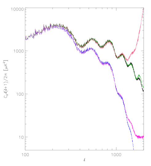
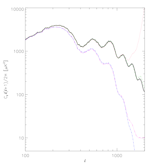
Figure 6: The two panels are identical except for the binning in $\ell$ in the right panel. No noise is considered. Angular power spectrum from the four considered patches. Solid (black) line: angular power spectrum of the input map without convolution; dash-three dots (fuxia): angular power spectrum of the map convolved with the simulated beam assuming the Planck scanning strategy; dots (red): angular power spectrum of the map convolved with the simulated beam assuming the Planck scanning strategy and divided by the symmetric beam window function; dashes (green): angular power spectrum of the deconvolved map; dash-dots (blue): angular power spectrum of the deconvolved map subsequently convolved with a symmetric beam with the effective resolution (see also the text).

3.4 Case D: application to Planck in the presence of noise

Analogously to the Case B (see Sect. 3.2) we have simulated four patches (of $1024^{2}$ pixels, as in the previous section) of instrumental uncorrelated Gaussian noise with $\sigma_{N}=9\mu$K (in terms of antenna temperature) for a pixel of $3.43^{\prime}$, as appropriate to the global Planck sensitivity at 100 GHz; for simplicity we have assumed a uniform noise.

This realization of noise map has been added to the map of signal and then method II has been applied to deconvolve the map of signal plus noise, as described in Sect. 3.2. We produced also four realizations of pure noise maps to be deconvolved in the same way. Finally, we generated another map of noise to be superimposed to the coadded map obtained from the convolution with the simulated beam including scanning strategy, for comparison.

We computed the angular power spectrum of the four maps of pure noise and of the four maps of pure noise deconvolved with method II. Fig. 7 (left panel) compares the averages of the four realizations of these power spectra and their relative variance (right panel). As evident, deconvolution increases the noise: a rough approximation of the ratio between of the noise angular power spectrum after deconvolution and before deconvolution is given by $\sim 2({\rm FWHM}/\Delta)^{2}{\rm exp}[(\sigma\ell/2)^{2}+(\sigma\ell/2)^{6}]$ where, as usual, ${\rm FWHM}=\sqrt{8{\rm ln}2}\sigma$ ($=10.68^{\prime}$) and $\Delta$ is the pixel side ($=3.43^{\prime}$). On the other hand, the relative variance of these power spectra is almost similar.

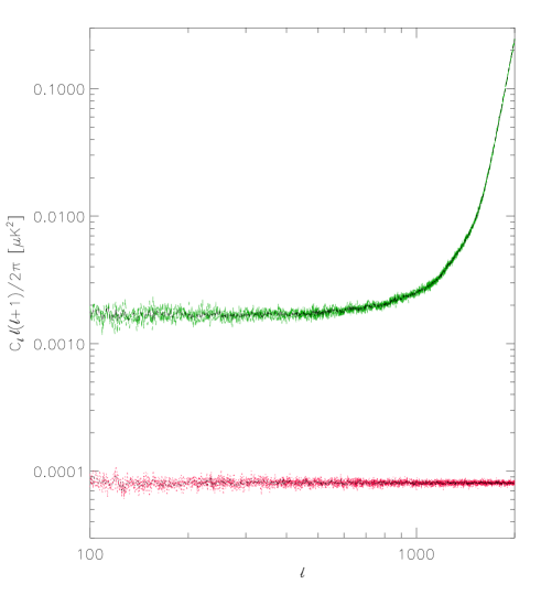
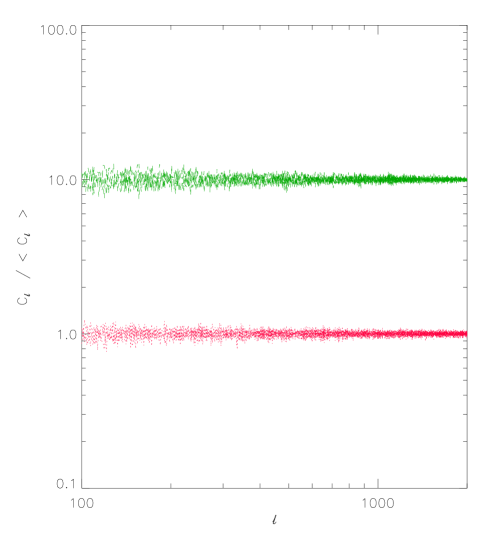
Figure 7: Left panel: comparison between the noise power spectrum before (red) and after (green) deconvolution for the four noise realizations (the inner (black) “curves” represent the two average noise power spectra). Right panel: ratio between the power spectrum of each of the four noise realizations and the average noise power spectrum, before and after deconvolution, multiplied by 10 in the latter case for graphic purposes (see also the text).

In spite of the relatively large increase of the noise power, we find that method II results to work quite well in removing the effect of main beam distortions up to the end of the fifth acoustic peak, when the average power spectrum of the deconvolved pure noise maps is subtracted to the power spectrum of the deconvolved noisy map (see the dashed (green) line in Fig. 8).

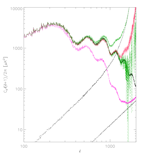
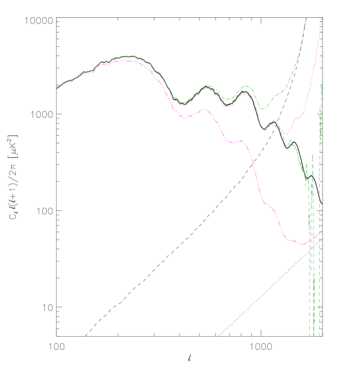
Figure 8: The two panels are identical except for the binning in $\ell$ in the right panel. The noise is included. Angular power spectrum from the four considered patches. Solid (black) line: angular power spectrum of the input map without convolution and without noise; dash-three dots (fuxia): angular power spectrum of the map convolved with the simulated beam assuming the Planck scanning strategy and adding a noise realization; dots (red): angular power spectrum of the map convolved with the simulated beam assuming the Planck scanning strategy and adding a noise realization, after the subtraction of the averaged power spectrum of four noise realizations and then divided by the symmetric beam window function; dotted (black) bottom line: averaged power spectrum of four noise realizations; dash-dots (green): angular power spectrum of the deconvolved map in the presence of a noise realization; dashes (green): angular power spectrum of the deconvolved map in the presence of a noise realization after the subtraction of the averaged power spectrum of four noise realizations deconvolved in the same way; dashed (black) bottom (at low $\ell$) line: averaged power spectrum of four noise realizations deconvolved in the same way (see also the text).

In Fig. 9 we report the relative (per cent) errors introduced by beam distortions in the absence of deconvolution, in the presence of deconvolution without applying the subtraction of the average deconvolved noise spectrum and by applying the deconvolution and the subtraction of average deconvolved noise spectrum. As evident, in the last case the power spectrum can be recovered with a good accuracy up to high multipoles (relative errors $\,\lower 2.0pt\hbox{${<\atop\hbox{\raise 4.0pt\hbox{$\sim$}}}$}\,5,10,15,20$ % respectively for $\ell\,\lower 2.0pt\hbox{${<\atop\hbox{\raise 4.0pt\hbox{$\sim$}}}$}\,1250,1470,1500,1650$ – see the dashed (green) line in the middle panel – to be compared with errors $\simeq 10,20,30$ % at $\ell\simeq 1200,1250,1300$ – see the dotted (red) line in the middle panel – and then dramatically increasing with $\ell$ in the absence of deconvolution). The right panel shows what already found for the noiseless case (Sect. 3.3): even by varying the assumed value of the symmetric beam width $\sigma$, an improvement in the $C_{\ell}$ recovery can not be reached simultaneously on the whole relevant range of multipoles.

Figure 9: The left and middle panels are identical except for the binning in $\ell$ in the middle panel. Errors in the angular power spectrum recovery from the four considered patches. Dash-three dots (fuxia): angular power spectrum of the map convolved with the simulated beam assuming the Planck scanning strategy and adding a noise realization; dots (red): angular power spectrum of the map convolved with the simulated beam assuming the Planck scanning strategy and adding a noise realization, after the subtraction of the averaged power spectrum of four noise realizations and then divided by the symmetric beam window function; dash-dots (blue): angular power spectrum of the deconvolved map in the presence of a noise realization; dashes (green): angular power spectrum of the deconvolved map in the presence of a noise realization after the subtraction of the averaged power spectrum of four noise realizations deconvolved in the same way. In the right panel we report the same line (dots, red) of the middle panel and four other power spectra obtained in similar way by assuming different values of effective angular resolution, with an effective FWHM increased or decreased by $0.05^{\prime}$ and $0.1^{\prime}$. Clearly, an improvement at $\ell\sim 400-800$ implies a worsening at $\ell\,\lower 2.0pt\hbox{${>\atop\hbox{\raise 4.0pt\hbox{$\sim$}}}$}\,1000$ and viceversa: therefore, even allowing for changes in the assumed effective angular resolution, the simple symmetric beam approximation can not improve the power spectrum recovery simultaneously in the two above ranges of $\ell$ (see also the text).

We have considered here for simplicity only equatorial patches. On the other hand, we have verified that the main beam distortion affects the reconstructed power spectrum in a similar way also on polar patches. In fact, even at high ecliptic latitudes a given pixel is preferentially observed with a limited number of beam orientations. In polar patches the Planck sensitivity is significantly better than the average. Therefore, in spite of the more complex data storage, deconvolution will be there less affected by the noise .

4 Discussion and conclusions

We have presented the basic formalism for a robust and feasible method for deconvolution in noisy CMB maps.

We have implemented and tested this method for two completely different situations: small patches observed with an elliptical beam and with a scanning strategy involving repeated measures of the same pixel but not related to a specific experiment and quite large sky areas observed with a realistic beam and a scanning strategy like that of the Planck satellite. A sensitivity level and a beam resolution typical of the Planck experiment at 100 GHz have been exploited.

After having verified the good accuracy of our deconvolution code to remove the main beam distortion effect in the angular power spectrum estimation in the absence of noise, we applied it to noisy maps. We demonstrate that it is possible to accurately evaluate the effect of deconvolution on pure noise simulated maps so deriving, with Monte Carlo simulations, a good estimation of the average deconvolved noise angular power spectrum to be subtracted from the deconvolved noisy maps.

In practice, for the considered sensitivity, $\simeq 9\mu$K for a pixel of $3.43^{\prime}$, and beam resolution, FWHM $\simeq 10^{\prime}-11^{\prime}$, our deconvolution code allows to efficiently remove the main beam distortion effect and accurately reconstruct the CMB power spectrum up to the end of the fifth acoustic peak.

Clearly, in the context of the Planck project, the measure of the very high multipole region of the CMB angular power spectrum will be take advantage from the cosmological frequency channels at highest resolution, namely the 217 GHz channel (having a FWHM $\simeq 5^{\prime}$), where Poisson fluctuations from extragalactic sources (see e.g. Toffolatti et al. 1998) are expected to be at a very low level and anisotropies from thermal Sunyaev-Zeldovich effects are, if not exactly null because of possible unbalanced contributions within the bandwidth, certainly very small. On the other hand, the frequency range about 100 GHz is where the global (Galactic plus extragalactic) foreground contamination is expected to be minimum. Therefore, it is extremely relevant to extract at these frequency an accurate estimation of the sky angular power spectrum, cleaned, as better as possible, from the all systematic effects. In addition, the removal of the main beam distortion effect, relevant at large multipoles, greatly helps the comparison between the results obtained at different frequency channels.

Of course, we plan to apply this method in the future also to lowest and highest beam resolutions and in the presence of other kinds of systematic effects. We believe that the results found here are very encouraging, suggesting that the main beam distortion effect, previously reduced by optimizing the optical design, can be further reduced in the data analysis.

Appendix A Transformation rules between Planck telescope frame and beam frame

Let $\@vec{s}$ be the unit vector, choosen outward the Sun direction, of the spin axis direction and $\hat{k}$ that of the direction, $z$, of the telescope line of sight (LOS), pointing at an angle $\alpha\sim 85^{\circ}$ from the direction of $\@vec{s}$.

On the plane tangent to the celestial sphere in the direction of the LOS we choose two coordinates $x$ and $y$, respectively defined by the unit vector $\hat{i}$ and $\hat{j}$ according to the convention that the unit vector $\hat{i}$ points always toward $\@vec{s}$ and that $x,y,z$ is a standard Cartesian frame, referred here as telescope frame.

Let $\hat{i}_{bf},\hat{j}_{bf},\hat{k}_{bf}$ be the unit vectors corresponding to the Cartesian axes $x_{bf},y_{bf},z_{bf}$ of the beam frame; $\hat{k}_{bf}$ defines the direction of the beam centre axis in the telescope frame. The beam frame is defined with respect to the telescope frame by three angles: $\theta_{B}$, $\phi_{B}$, $\psi_{B}$ ($\theta_{B}$ and $\phi_{B}$, two standard polar coordinates defining the direction of the beam centre axis, range respectively from $0^{\circ}$, for an on-axis beam, to some degrees, for LFI off-axis beams, and from $0^{\circ}$ to $360^{\circ}$).

Let $\hat{i^{\prime}}_{bf},\hat{j^{\prime}}_{bf},\hat{k^{\prime}}_{bf^{\prime}}$ ($\hat{k^{\prime}}_{bf}=\hat{k}_{bf}$) be the unit vectors corresponding to the Cartesian axes $x^{\prime},y^{\prime},z^{\prime}$ of an intermediate frame, defined by the two angles $\theta_{B}$ and $\phi_{B}$, obtained by the telescope frame $x,y,z$ when the unit vector of the axis $z$ is rotated by an angle $\theta_{B}$ on the plane defined by the unit vector of the axis $z$ and the unit vector $\hat{k}_{bf}$ up to reach $\hat{k}_{bf}$:

$$\hat{k^{\prime}}_{bf}=\hat{k}_{bf}={\rm cos}(\phi_{B}){\rm sin}(\theta_{B})\hat{i}+{\rm sin}(\phi_{B}){\rm sin}(\theta_{B})\hat{j}+{\rm cos}(\theta_{B})\hat{k}$$ (12)

$$\hat{i^{\prime}}_{bf}=[{\rm cos}(\phi_{B})^{2}{\rm cos}(\theta_{B})+{\rm sin}(\phi_{B})^{2}]\hat{i}+[{\rm sin}(\phi_{B}){\rm cos}(\phi_{B})({\rm cos}(\theta_{B})-1)]\hat{j}-{\rm sin}(\theta_{B}){\rm cos}(\phi_{B})\hat{k}$$ (13)

$$\hat{j^{\prime}}_{bf}=[{\rm sin}(\phi_{B}){\rm cos}(\phi_{B})({\rm cos}(\theta_{B})-1)]\hat{i}+[{\rm cos}(\theta_{B}){\rm sin}(\phi_{B})^{2}+{\rm cos}(\phi_{B})^{2}]\hat{j}-{\rm sin}(\theta_{B}){\rm sin}(\phi_{B})\hat{k}\,.$$ (14)

The beam frame is obtained from the intermediate frame through a further (anti-clockwise) rotation of an angle $\psi_{B}$ (ranging from $0^{\circ}$ to $360^{\circ}$ ) around $\hat{k}_{bf}$ and is therefore explicitely given by:

$$\hat{i}_{bf} = [{\rm cos}(\psi_{B})\hat{i^{\prime}}_{bf,x}+{\rm sin}(\psi_{B})\hat{j^{\prime}}_{bf,x}]\hat{i}+[{\rm cos}(\psi_{B})\hat{i^{\prime}}_{bf,y}+{\rm sin}(\psi_{B})\hat{j^{\prime}}_{bf,y}]\hat{j}$$ (15)

$$+[{\rm cos}(\psi_{B})\hat{i^{\prime}}_{bf,z}+{\rm sin}(\psi_{B})\hat{j^{\prime}}_{bf,z}]\hat{z}$$

$$\hat{j}_{bf} = [-{\rm sin}(\psi_{B})\hat{i^{\prime}}_{bf,x}+{\rm cos}(\psi_{B})\hat{j^{\prime}}_{bf,x}]\hat{i}+[-{\rm sin}(\psi_{B})\hat{i^{\prime}}_{bf,y}+{\rm cos}(\psi_{B})\hat{j^{\prime}}_{bf,y}]\hat{j}$$ (16)

$$+[-{\rm sin}(\psi_{B})\hat{i^{\prime}}_{bf,z}+{\rm cos}(\psi_{B})\hat{j^{\prime}}_{bf,z}]\hat{z}\,,$$

where the bottom index $x$ $(y,z)$ indicates the component of intermediate frame unit vector along the axis $x$ $(y,z)$ of the telescope frame, as defined by eqs. (A1–A3).

References

- (1) Arnau, J.V., & Sáez, D., 2000, New Astron., 5, 121
- (2) Arnau, J.V., Aliaga, A.M., Sáez, D., 2002, A&A, 382, 1138
- (3) Bernard, J.P., Puget, J.L., Sygnet, J.F., Lamarre, J.M., 2002, Draft note on HFI’s view on Planck Scanning Strategy, Technical Note PL-HFI-IAS-TN-SCAN01, 0.2.1
- (4) Bersanelli, M. et al. 1996, ESA, COBRAS/SAMBA Report on the Phase A Study, D/SCI(96)3
- (5) Bond, J.R., & Efstathiou, G., 1987, MNRAS, 226, 655
- (6) Burigana, C., Malaspina, M., Mandolesi, N. et al. 1997, Int. Rep. TeSRE/CNR 198/1997, November, astro-ph/9906360
- (7) Burigana, C., Maino, D., Mandolesi, N. et al. 1998, A&AS, 130, 551
- (8) Burigana, C., Maino, D., Mandolesi, N. et al. 2000a, Astroph. Lett. Comm., 37, 253
- (9) Burigana, C., Maino, D., Natoli, P. et al. 2000, Straylight effects and beam reconstruction in Planck/LFI observations, talk at the “Planck Scanning Strategy Meeting”, Villa Mondragone - Monteporzio Catone (Roma), Italy, 22-23 June 2000
- (10) Burigana, C., Maino, D., Gòrski, K.M. et al. 2001, A&A, 373, 345
- (11) Burigana, C., Natoli, P., Vittorio, N., Mandolesi, N., Bersanelli, M., 2002, Exp. Astron., 12/2, 87, 2001
- (12) Burigana, C., Sandri, M., Villa, F. et al. 2003, A&A, submitted
- (13) Delabrouille, J., 1998, A&ASS, 127, 555
- (14) Fosalba, P., Dore, O., Bouchet, F.R., 2002, Phys. Rev. D, 65, 063003
- (15) Górski, K.M., Hivon, E., Wandelt, B.D., 1999, “Proceedings of the MPA/ESO Conference on Evolution of Large-Scale Structure: from Recombination to Garching”, ed. Banday A.J., Sheth R.K., Da Costa L., pg. 37, astro-ph/9812350
- (16) Lama, N., C. Vuerli, C., Pasian, F., A Pipeline Oriented Data Management System: Design and Implementation with an Object-Oriented Database, to be published (in electronic form) in the Memorie della Sait-Supplementi, http://www.ts.astro.it/sait2003/posters.html
- (17) Maino, D., Burigana, C., Maltoni, M. et al. 1999, A&AS, 140, 383
- (18) Maino, D., Burigana, C., Gòrski, K.M., Mandolesi, N., Bersanelli, M., 2002, A&A, 387, 356
- (19) Mandolesi, N. et al. 1998, Planck LFI, A Proposal Submitted to the ESA
- (20) Mandolesi, N., Bersanelli, M., Burigana, C., Villa, F., 2000a, Astroph. Lett. Comm., 37, 151
- (21) Mandolesi, N., Bersanelli, M., Burigana, C. et al. 2000b, A&AS, 145, 323
- (22) Mennella, A., Bersanelli, M., Burigana, C., et al., 2002, A&A, 384, 736
- (23) Natoli, P., de Gasperis, G., Gheller, C., Vittorio, N., 2001, A&A, 372, 346
- (24) Natoli, P., Marinucci, D., Cabella, P., de Gasperis, G., Vittorio, N., 2002, A&A, 383, 1100
- (25) Page, L., Barnes, C., Hinshaw, G. et al. 2003, ApJ, submitted, astro-ph/0302214
- (26) Puget, J.L. et al. 1998, HFI for the Planck Mission, A Proposal Submitted to the ESA
- (27) Sáez, D., & Arnau, J.V., 1997, ApJ, 476, 1
- (28) Sáez, D., Holtmann, E., & Smoot, G.F., 1996, ApJ, 473, 1
- (29) Sandri, M., Bersanelli, M., Burigana, C. et al. 2002, in “Experimental Cosmology at millimetre wavelengths – 2K1BC Workshop”, Breuil-Cervinia (AO), Valle d’Aosta, Italy, 9-13 July 2001, AIP Conference Proc. 616, De Petris M., Gervasi M., (Eds.), pg. 242
- (30) Sandri, M., Villa, F., Nesti, R. et al. 2003, A&A, to be submitted
- (31) Seiffert, M., Mennella, A., Burigana, C. et al. 2002, A&A, 391, 1185
- (32) Seljak, U., & Zaldarriaga, M., 1996, ApJ, 469, 437
- (33) Tauber, J. A., “The Planck Mission”, in The Extragalactic Infrared Background and its Cosmological Implications, Proceedings of the IAU Symposium, Vol. 204, 2000, M. Harwit and M. Hauser, eds.
- (34) Toffolatti, L., Argüeso Gómez, F., De Zotti, G. et al. 1998, MNRAS, 297, 117
- (35) Villa, F., Mandolesi, N., Burigana, C., 1998, Int. Rep. TeSRE/CNR 221/1998, September