WMAP and the Generalized Chaplygin Gas

Abstract

We compare the WMAP temperature power spectrum and SNIa data to models with a generalized Chaplygin gas as dark energy. The generalized Chaplygin gas is a component with an exotic equation of state, $p_{X}=-A/\rho^{\alpha}_{X}$ (a polytropic gas with negative constant and exponent). Our main result is that, restricting to a flat universe and to adiabatic pressure perturbations for the generalized Chaplygin gas, the constraints at 95% CL to the present equation of state $w_{X}=p_{X}/\rho_{X}$ and to the parameter $\alpha$ are $-1\leq w_{X}<-0.8$, $0\leq\alpha<0.2$, respectively. Moreover, we show that a Chaplygin gas ($\alpha=1$) as a candidate for dark energy is ruled out by our analysis at more than the $99.99\%$ CL. A generalized Chaplygin gas as a unified dark matter candidate $(\Omega_{CDM}=0)$ appears much less likely than as a dark energy model, although its $\chi^{2}$ is only two sigma away from the expected value.

1 Introduction

The picture of a universe mostly filled by an unknown component, Dark Energy (DE henceforth), seems overwhelmingly justified by the latest observations of CMB anisotropies (Spergel et al. 2003).

While there is a strong degeneracy of the multitude of DE candidates for the background evolution – and therefore in the SNIa data (Perlmutter et al. 1999; Riess et al. 1998) –, additional information should be contained in the linear fluctuations. However, in order to differentiate among DE models, the avenue of studying DE fluctuations is not promising as it seems. Infact, in the simplest uncoupled quintessence models (Ratra & Peebles 1988; Frieman et al. 1995; Caldwell, Dave & Steinhardt 1995) based on scalar fields with ordinary Klein-Gordon Lagrangian, quintessence fluctuations are evanescent on sub-horizon scales. This is due to the presence of a Jeans scale for scalar field perturbations, of the order of the Hubble radius. This Jeans scale is related to a unitary sound speed (in $c=1$ units) for scalar field perturbations. For the same reason, isocurvature perturbations caused by an offset of the quintessence component (Abramo & Finelli 2001) are not observationally harmful as other isocurvature modes.

A possibility of having a smaller Jeans scale for dark energy fluctuations is offered by theories with non standard kinetic terms for the scalar field candidate. A scalar field with a Born-Infeld action is an example:

$$S=\int d^{4}x\sqrt{-g}\,V\,\sqrt{1+\frac{\partial_{\mu}\varphi\partial^{\mu}\varphi}{M^{4}}}\,,$$ (1)

where $M$ is a fundamental scale and $V$ is a potential. Recently, the tachyon field (with $V=V(\varphi)$) motivated from string theory has received a lot of attention (Sen 2002, Gibbons 2002, Padmanabhan 2002). A Chaplygin gas is a hydrodinamical description of the scalar field with the Born-Infeld Lagrangian in Eq. (1) with constant $V$ (Kamenshchik, Moschella & Pasquier 2001). A Chaplygin gas is characterized by a pressure which is inversely proportional to the energy $p\propto-1/\rho$. A generalized Chaplygin gas (henceforth GCG) is a perfect fluid with a polytropic equation of state (Bento, Bertolami & Sen 2002):

$$p_{X}=-\frac{A}{\rho_{X}^{\alpha}}$$ (2)

where $\alpha$ is a parameter between $0$ and $1$ in order to have a sound speed at most luminal for perturbations. $A$ is a constant with dimensions $[M^{4(1+\alpha)}]$. A GCG is a phenomenological extension of the Chaplygin gas, which exhausts all the possibilities for a polytropic perfect fluid dark energy candidate, whose perturbations are stable on small scales (Fabris, Goncalves & Souza 2002a, Carturan & Finelli 2002 – henceforth CF –).

The behaviour in time of a GCG interpolates between dust and a cosmological constant, with an intermediate behaviour as $p=\alpha\rho$. The Jeans instability of GCG perturbations is first similar to CDM fluctuations (when the GCG has a negligible pressure) and then disappears (when the GCG behaves as a cosmological constant) (see CF). Both this late suppression of GCG fluctuations and the apperance of a non zero Jeans length leave a large integrated Sachs-Wolfe (ISW) imprint on the CMB anisotropies (CF). A model in which the GCG is the only dark component is referred to as a unified dark matter/dark energy (UDM) model.

The viability of GCG as DE and UDM model has been first analyzed in the context of Supernovae (Fabris et al. 2002b; Avelino et al. 2002; Makler, de Oliveira & Waga 2003) and other complementary data (Dev, Jain & Alcaniz 2003, Alcaniz, Jain and Dev 2003). The comparison with CMB data has been the next step (CF, Bean & Dore’ 2003) and it has led to much stronger constraints (Bean & Dore’ 2003).

The imprint of a GCG is also present on the matter power spectrum, since GCG perturbations affect both CMB anisotropies and structure formation. This last issue has been considered by Sandvik et al. (2002) in the context of UDM models, claiming that a GCG is ruled out as a UDM candidate at $99.999\%$ (Sandvik et al. 2002). However, their analysis does not take into account baryons, while we will show they are relevant for the shape of the total matter power spectrum. Moreover, the analysis by Sandvik et al. is based on a linear treatment of perturbations until the present time, neglecting any non linear effects which may be important and unexpected because of the time dependence of the GCG Jeans length. Such nonlinear effects should be more important for the present matter power spectrum than for the CMB spectrum. For this reason, we focus on the comparison with CMB data.

In this paper we compare the predictions of GCG models with the recently released WMAP data, which provide the most precise determination of the CMB spectrum so far (Hinshaw et al. 2003), and with SNIa data (Perlmutter et al. 1999, Riess et al. 1998).

2 The Model

In this section we review a brief and basic description of the model (for more details see CF). The conservation equation for the GCG in a Robertson-Walker metric is solved by

$$\rho_{X}=[A+\frac{B}{a^{3(\alpha+1)}}]^{\frac{1}{1+\alpha}},$$ (3)

where $a$ is the scale factor ($a=1$ today) and $B$ is an integration constant with dimension $[M^{4(1+\alpha)}]$.

The equation of state is therefore

$$w_{X}(a)=\frac{p_{X}}{\rho_{X}}=-\frac{A}{\rho_{X}^{1+\alpha}}\,,$$ (4)

while the present equation of state is

$$w_{X}=-\frac{A}{A+B}.$$

Instead of $A,B$ we find convenient to employ the parameters $\Omega_{X},w_{X}$ , where $\Omega_{X}$ is the present value of the density parameter of the GCG and

$$A = -w_{X}(\Omega_{X}\rho_{c})^{1+\alpha},$$

$$B = (1+w_{X})(\Omega_{X}\rho_{c})^{1+\alpha},$$

where $\rho_{c}$ is the present critical density. Beside the GCG we introduce for generality also baryons and CDM. Although the GCG is very interesting as an unified model of dark energy and dark matter, it is conceivable that it is in fact only a DE component additional to ordinary CDM and baryons.

Perturbations of GCG are stable on small scales since the sound speed is positive ($c_{X}^{2}=\partial p_{X}/\partial\rho_{X}=-\alpha w_{X}$). An important consequence of assuming a perfect fluid instead of a scalar field as a candidate of dark energy is the absence of intrinsic non adiabatic pressure perturbations. Infact, for a GCG pressure perturbations are locked to density perturbations

$$\delta p_{X}=c_{X}^{2}\delta\rho_{X}\,.$$ (5)

Instead, in presence of non adiabatic pressure perturbations, we have in general:

$$\delta p_{X}=c_{X}^{2}\delta\rho_{X}+\Delta p_{X}\,.$$ (6)

For example, in a scalar field model with standard kinetic term for quintessence $c_{X}^{2}=1$ and $\Delta p_{X}=2V_{\phi}\delta\phi$, where $V_{\phi}$ is the first derivative of the potential and $\delta\phi$ is the field fluctuation.

A perfect fluid description of a GCG offers the chance to explore the possibility of the basic relation (5) for dark energy pressure perturbations.

In Figs. 1 and 2 we compare the $C_{\ell}$ temperature spectrum with the WMAP data varying $w_{X}$ and $\alpha$, respectively (see also CF). These figures show how strongly the $C_{\ell}$ spectrum depends on perturbations of GCG, when this is a DE candidate ($\Omega_{c}$ is fixed to $0.27$). Fig. 1 shows how the resulting CMB spectrum strongly differ even for models which have $w_{X}\leq-0.91$. Notice that the 2nd and 3rd peak move to the left increasing $w_{X}$, because then the expansion is less and less accelerated, while the 1st peak remains more or less stable because of the concurring strong integrated Sachs-Wolfe (ISW) effect. Fig. 2 shows the strong dependence of CMB spectrum on $\alpha$, which regulates the Jeans length of GCG perturbations and therefore the amount of ISW effect. The peak-to-plateau ratio decreases for $\alpha$ increasing, because after the dust behaviour the GCG induces a strong ISW. The dependence of CMB spectrum and LSS on the Jeans length of DE perturbations is a generic effect and it has been also found recently in K-essence models (DeDeo, Caldwell & Steinhardt 2003), but it is less severe than in GCG models.

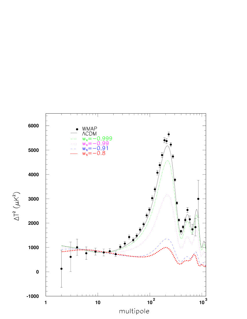
Figure 1: The $C_{\ell}$ spectrum varying $w_{X}$ is plotted in comparison with a $\Lambda$CDM model (the upper curve): $w_{X}\simeq-0.8,-0.91,-0.99,-0.999$ from bottom to top, respectively. The other parameters are $\alpha=1$, $h=0.72$, $w_{b}=0.024$, $w_{c}=0.14$, $n_{s}=1$. The spectra are COBE normalized at $\ell=10$.

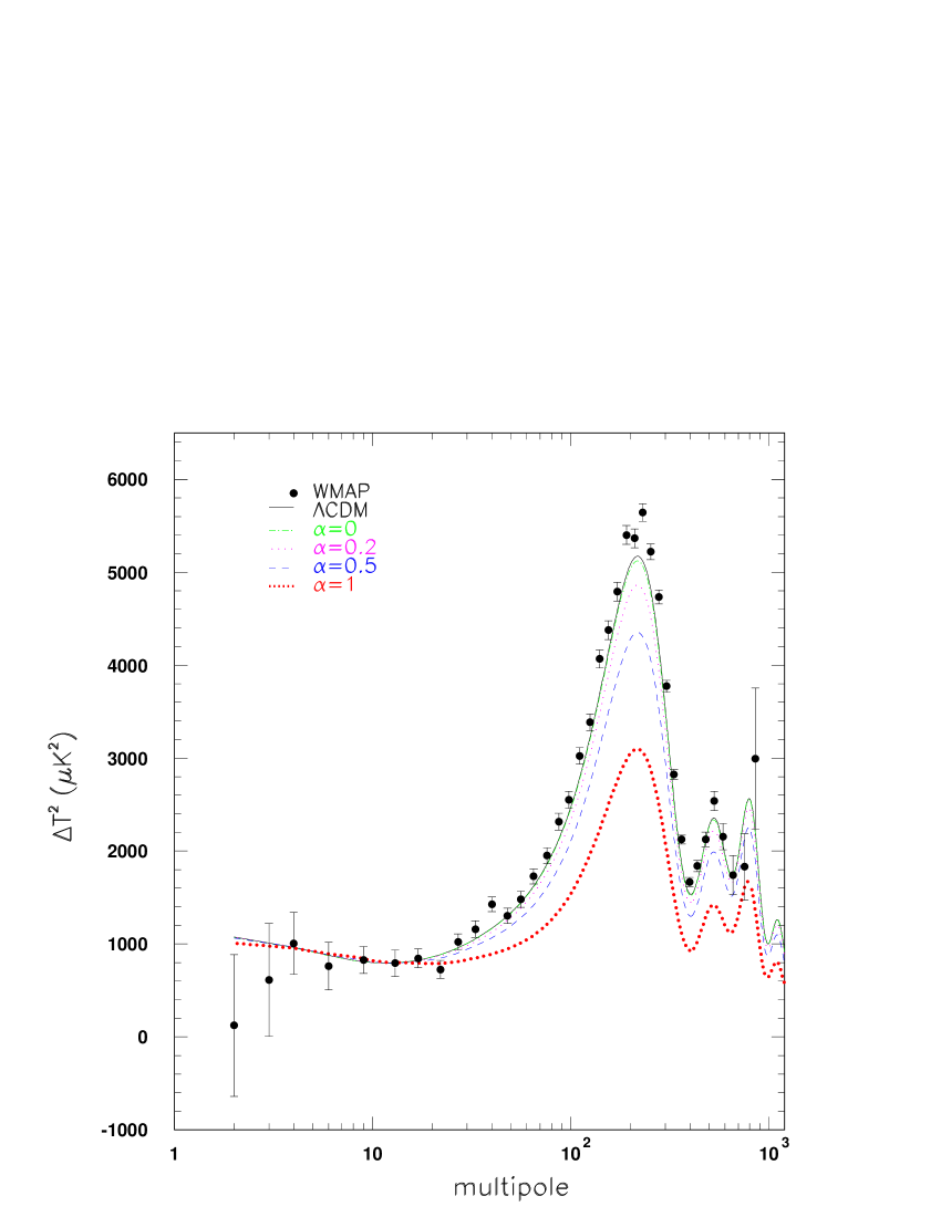
Figure 2: The $C_{\ell}$ spectrum varying $\alpha$ is plotted in comparison with a $\Lambda$CDM model (the upper solid line): $\alpha=1,0.5,0.2,0$ from bottom to top, respectively. The other parameters are $w_{X}\simeq-0.99$, $h=0.72$, $w_{b}=0.024$, $w_{c}=0.14$, $n_{s}=1$. The spectra are COBE normalized at $\ell=10$. We note how the $\Lambda$CDM curve and $\alpha=0$ are very close, but not identical because of the different perturbation sectors.

3 Likelihood analysis

We compare the models to the combined power spectrum estimated by WMAP (Hinshaw et al. 2003). To derive the likelihood we adopt a version of the routine described in Verde et al. (2003), which takes into account all the relevant experimental properties (calibration, beam uncertainties, window functions, etc). Since the likelihood routine employs approximations that work only for spectra not too far from the data, we run it only for models whose $\chi^{2}$ per d.o.f. is less than 1.5 from the number of degrees of freedom.

Our theoretical model depends on two GCG parameters, four cosmological parameters and the overall normalization $N$:

$$\alpha,w_{X},n_{s},h,\omega_{b},\omega_{c},N.$$ (7)

where $\omega_{b,c}=\Omega_{b,c}h^{2}$ and $n_{s}$ is the primordial fluctuation slope. As anticipated, to save computing time we found necessary to restrict the analysis to a flat space; moreover, we fixed the optical depth to $\tau=0.17$, the mean value found by WMAP (Spergel et al. 2003). The overall normalization has been integrated out numerically. We calculate the theoretical $C_{\ell,t}$ spectra by a modified parallelized CMBFAST (Seljak & Zaldarriaga 1996) code that includes the full set of perturbation equations (see CF). We do not include gravitational waves and the other parameters are set as follows: $T_{cmb}=2.726K,$ $Y_{He}=0.24,N_{\nu}=3.04$.

We evaluated the likelihood on a non-uniformly spaced grid of roughly $50,000$ models (for each normalization) with the following top-hat broad priors: $w_{X}\in(-1,-0.5),$ $\quad\alpha\in(0,.5),\quad$ $n_{s}\in(0.8,1.2),$ $\quad\omega_{b}\in(0.005,0.04),\quad$ $\omega_{c}\in(0.0,0.2)$. For the Hubble constant we adopted the top-hat prior $h\in(0.5,0.9);$ we also employed the HST result (Freedman et al. 2001) $h=0.72\pm 0.08$ (Gaussian prior). One reason to adopt a grid approach than a Markov chain method (as in Verde et al. 2003) is that the independent grid evaluation can be parallelized with maximum efficiency.

4 Results from comparison with WMAP

In Fig. 3 we plot the likelihood functions for each parameter, marginalizing in turn over the others. The horizontal lines mark the 68% and 95% CL; the vertical lines the 68% and 95% upper bounds. We obtain the bounds

$$\alpha < 0.2(0.05)$$

$$w_{x} < -0.8(-0.92)$$ (8)

at 95%(68%) CL. These constraints are the most stringent ones obtained so far using only CMB data; the limit on $\alpha$ is 5–10 stronger than the previous one obtained with pre-WMAP data (Bean & Dore’ 2002). For the other parameters we obtain results not very different than the standard ones. We also show the results imposing the HST prior $h=0.72\pm 0.08$; they are almost identical to the one without prior on $h$. The best fit DE model is $n_{s}=1$, $\alpha=0$, $w_{X}=-0.98$, $h=0.71$, $\omega_{b}=0.024$, $\omega_{c}=0.12$ has $\chi^{2}$/d.o.f.=979/892.

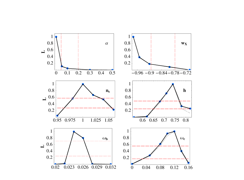
Figure 3: Marginalized likelihood functions for the six cosmological parameters. The dotted lines are for the HST prior on the Hubble constant. The horizontal long-dashed lines are the confidence levels at 68% and 95%. The vertical long-dashed lines in the panels for $\alpha\,,w_{X}$ mark the upper bounds at 68% and 95% CL.

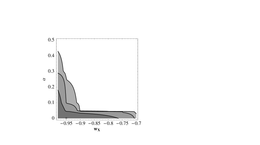
Figure 4: Likelihood in the plane $w_{X},\alpha$. The contours are at the 68%, 95% and 99% CL, inside to outside.

5 Constraints on the Unified Dark Model

Any DE model which interpolates in time between a dust epoch and an accelerating stage has the possibility of playing the role of a UDM candidate, if one renounces to the presence of CDM. Naturally, in such a case one should explain also why 30% or so of the matter collapsed into galaxies and clusters while the remaining did not. The GCG has received a lot of attention also in this light of a UDM model. While SNIa data allow for this possibility, it was claimed that LSS data completely ruled it out (Sandvik et al. 2002). Here we find that WMAP data alone (for which a linear analysis is sufficient) show that a GCG as a unified candidate is much less likely than a model which includes a CDM component. The likelihood for $\omega_{c}=0$ is infact roughly 50 times smaller than for $\omega_{c}=0.12$; formally, this rules out the UDM at slightly more that 99.99% C.L. when compared with GCG as DE. The lowest value allowed by WMAP data is 0.1 (95C.L.). However, if we calculate the $\chi^{2}$ for the best fit among the UDM cases (corresponding to a model with $n_{s}=0.98$, $\alpha=0$, $w_{X}=-0.8$, $h=0.82$, $\omega_{b}=0.026$) we find $\chi^{2}$/d.o.f.=986/893, indicating that the UDM model is an acceptable fit to WMAP data at at 2$\sigma$ level.

Note that our results have been obtained varying also $n_{s}$, which has been instead fixed in the analysis of Bean & Dore’ (2002) and of Sandvik et al. (2002) (who also fixed $h$).

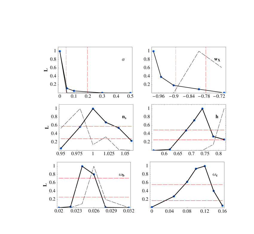
Figure 5: Likelihood functions for the GCG model (full curve) and the unified model ($\Omega_{c}=0$ ; dashed curve). The horizontal long-dashed lines are the confidence levels at 68% and 95%. The vertical long-dashed lines in the panels for $\alpha\,,w_{X}$ mark the upper bounds at 68% and 95% CL.

6 Adding the Supernovae constraints

We now proceed with a further refinement of our result, by taking into account the constraint from the SN I a Hubble diagram. This has been evaluated by several groups (Fabris et al. 2002a; Avelino et al. 2002; Makler et al. 2003), but not in a suitable form for our purposes.

The luminosity distance in a GCG model in flat space is

$$d_{L}(z)=(1+z)\int_{0}^{z}\frac{dz^{\prime}}{H(z^{\prime})},$$

where the Hubble function is

$$H^{2}(z)=H_{0}^{2}\left[\Omega_{m}(1+z)^{3}+(1-\Omega_{m})((1+w_{X})(1+z)^{3(1+\alpha)}-w_{X})^{\frac{1}{1+\alpha}}\right],$$

and $\Omega_{m}=\Omega_{b}+\Omega_{c}$.

We compare the luminosity distance to the SCP data of Perlmutter et al. (1999) (their fit C), to which we add the supernova at $z\approx 1.7$ (Benitez et al. 2002). We show in Fig. 6 the 2-dimensional likelihood function marginalized over the “nuisance parameters” (see definitions in Perlmutter et al. 1999) $\alpha,M^{*}$ , and over $\Omega_{m}$ with Gaussian prior $\Omega_{m}=0.3\pm 0.1$. Notice that the contours are almost insensitive to $\alpha\,$ since $d_{L}(z)$ at small redshifts is independent of $\alpha$. This shows how CMB data constrain the GCG models much more than SNIa data. In Fig. 7 we multiply the SN and WMAP likelihood functions. The final constraints turn out to be almost identical to those in (8).

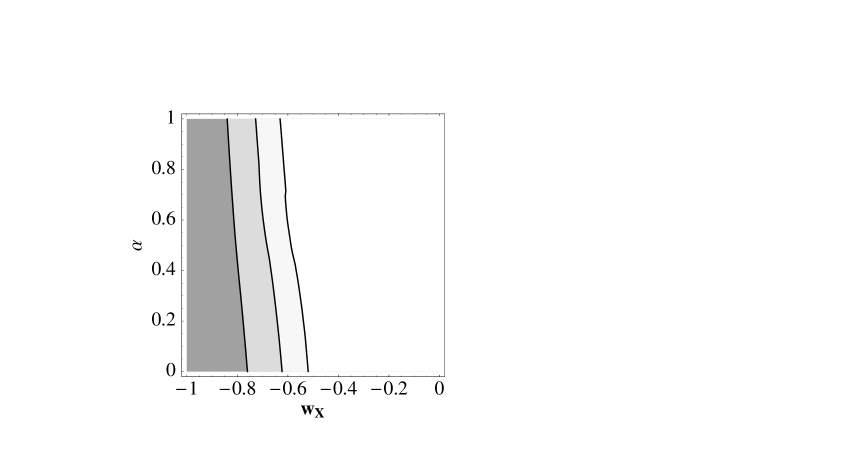
Figure 6: SNIa likelihood in the plane $w_{X}\,,\alpha$, with a Gaussian prior $\Omega_{m}=0.3\pm 0.1$. Confidence regions at 65%, 95% and 99% from dark to light gray.

Figure 7: Adding the SNIa constraint. The thick gray curves are the confidence regions for the SNIa; the dotted curves the confidence regions for the CMB; the gray regions represent the combined likelihood (65% and 95% c.l.). As it can be seen, the SNIa constraints add little information.

7 Considerations on the Mass Power Spectrum

The influence of the GCG on structure formation is another important observational imprint of this candidate for DE and UDM model. GCG fluctuations accumulate on all scales when the GCG behaves as CDM. As soon as the GCG equation of state drops below zero, the GCG fluctuations are no longer Jeans unstable at all scales, oscillating and decaying. This exotic behaviour of fluctuations occurs also when the GCG simulates $\Lambda$. As already said in the introduction, this suppression of fluctuations is in part responsible for the large ISW effect in CMB anisotropies. It is clear that a similar behaviour of fluctuations differs both from CDM and standard quintessence, and it is more important in absence of CDM, i.e. in a UDM model.

Sandvik et al. (2002) used a comparison of the predicted power spectrum in GCG models with LSS data – 2dF survey (Colless et al. 2001; see also Tegmark, Hamilton & Xu 2002) – to rule out the GCG as a UDM candidate at 99.999% CL. Their approximate analysis neglects baryons (this has also been noted recently by Beca et al. 2003) and is based on a linear treatment of perturbations until the present time. However, the nonlinear clustering of GCG could be rather nontrivial because of the time dependence of its Jeans length and deserves more study.

In Fig. 8 we compare the predicted power spectra – total (solid line), GCG (dashed line) and baryon (dotted line) – for UDM model with the APM (Padilla & Baugh 2003) and 2dF (Colless et al. 2001) data when $\alpha$ varies. The power spectra are obtained through the transfer functions of the modified CMBFAST code (CF), i.e. by using the linear evolution. We do not show as target the CDM power spectrum because almost indistinguishable from the baryon one. The power spectra are normalized at $k=0.01$ h/Mpc as in Sandvik et al. (2002) and the results in Fig. 8 can be directly compared with those of Fig. 1 in Sandvik et al.. It is very interesting to note the role of baryons, which were neglected by Sandvik et al.: baryons keep on clustering on all scales, at all time after decoupling. Even if baryons are a subdominant component ($\Omega_{b}=0.05$), they are very important when one considers the total matter power spectrum $P_{T}(k)=\Omega_{b}^{2}P_{b}(k)+\Omega_{X}^{2}P_{X}(k)$. The inclusion of baryons smooths out the oscillations of the GCG component in the total matter power spectrum, in particular for $\alpha\geq 10^{-3}$: when comparing to the LSS data, only the shape is relevant and not the features of the GCG component. We also note that for $\alpha\geq 10^{-2}$ the appearance of a finite Jeans length and/or of a suppression of DE component maybe very interesting in connection with the bump present in APM data. Therefore, it appears that an intermediate value of $\alpha$ ($0.01\leq\alpha\leq 0.2$) may fit both CMB and LSS data.

On concluding, in UDM models the comparison of the total matter power spectrum with LSS changes by including baryons, even within the linear approximation. In the context of DE models, this effect is even more important since CDM perturbations clustering on all scales are also present.

Figure 8: We compare the predictions of a UDM model based on GCG with APM (diamonds) and 2dF (asterisks) surveys when $\alpha$ varies ($\alpha=10^{-5},10^{-4},10^{-3},10^{-2},0.05,0.25$ from left to right, top to bottom). The other parameters are $h=0.7$, $w_{X}\simeq-0.74$, $\Omega_{X}=0.95$ and $\Omega_{b}=0.05$.

8 Conclusions

We have analyzed quantitatively the observational effects of a GCG as a DE candidate. We have restricted our analysis to a flat universe and to purely adiabatic pressure perturbations.

So far, most authors studied only the comparison of the Hubble law predicted in presence of a GCG with the SNIa (Fabris et al. 2002a; Avelino et al. 2002; Makler et al. 2003). However, as also our Figs. 6–7 show, SNIa data constrain GCG models very weakly. For instance, the Hubble law is almost insensitive to $\alpha$, as we see in Fig. 6. Instead, $\alpha$ is the maximum value which the sound speed can reach and it is related to the time at which the Jeans instability disappears and therefore fluctuations are very sensitive to this quantity: this results in a strong dependence of the CMB spectrum on $\alpha$, as we see from Fig. 2.

The combined result of CMB and SNIa data is presented in Fig. 7, which leads to $\alpha<0.2$ and $w_{X}<-0.8$ at $95\%$ c.l. The bound imposed by WMAP data on $\alpha$ is 5–10 stronger than the previous data (Bean & Dore 2003), and the Chaplygin gas ($\alpha=1$) is ruled out as a DE candidate at more than the $99.99\%$ c.l.

The possibility of a unified dark model with a GCG (corresponding to $\Omega_{c}=0$) seems disfavoured by the latest CMB anisotropy data in comparison to the GCG playing the role of a DE model, although the UDM on its own is not a bad fit to the data. The $\chi^{2}$ statistics is 987/893 for a UDM model, whereas is 979/892 for a DE model. Our result is in contrast with the analysis of the peaks position recently performed by Bento, Bertolami and Sen (2003), in which a different region in the ($\alpha\,,w_{X}$) plane is allowed. This disagreement may come from an inaccurate analytic estimate of the peaks position (already pointed out by CF).

We have also addressed the problem of the comparison with the LSS data. We have compared results on the matter power spectrum with 2dF and APM data, within the linear approximation. By considering the worst case, i.e. a UDM model, we find that LSS data may be complementary to CMB data. The main question about the validity of linear treatment on such short scales however remains.

On concluding, standard quintessence models seem the most economic variation of DE models with respect to $\Lambda$CDM. Differentiating among DE models by studying the sound speed of its perturbations seems a promising avenue and this has already been shown in two different class of models (CF; DeDeo et al. 2003). We have shown that GCG models are models with high predictive power when compared with CMB anisotropies. Current and future  high precision CMB anisotropy data can finally constrain and/or rule out physical scenarios based on different models of DE.

References

- [] Abramo R., Finelli F., 2001, Phys. Rev. D, 64, 083513
- [] Alcaniz J.S., Jain D., Dev A., 2003, Phys. Rev. D, 67, 043514
- [] Avelino P.P., Beca L.M.G., de Carvalho, J.P.M., Martins, C.J.A.P., Pinto P., 2002, Phys. Rev. D, 66, 043507
- [] Bean R., Dore O., 2003, arXiv astro-ph/0301308
- [] Beca L.M.G., Avelino P.P., de Carvalho J.P.M., Martins C.J.A.P., 2003, arXiv astro-ph/0303564
- [] Benitez N. et al., 2002, ApJ, 577, L1
- [] Bento M.C., Bertolami O., Sen A.A., 2002, Phys. Rev. D, 66, 043507
- [] Bento M.C., Bertolami O., Sen A.A., 2003, arXiv astro-ph/0303538
- [] Caldwell R.R., Dave R., Steinhardt P.J., 1995, PRL, 75, 2077
- [] Carturan D., Finelli F., 2002, arXiv astro-ph/0211626
- [] Colless M. et al., 2001, MNRAS, 328, 1039
- [] DeDeo S., Caldwell R.R., Steinhardt P.J., 2003, arXiv astro-ph/0301284
- [] Dev A., Jain D., Alcaniz J.S., 2003, Phys. Rev. D, 67, 023515
- [] Fabris J.C., Goncalves S.V.B., de Souza P.E.V., 2002a, Gen. Rel. Grav., 34, 53
- [] Fabris J.C., Goncalves S.V.B., de Souza P.E.V., 2002b, arXiv astro-ph/0207430
- [] Freedman W.L. et al., 2001, ApJ, 553, 47
- [] Frieman J., Hill C., Stebbins A., Waga I., 1995, Phys. Rev. Lett. 75, 2077
- [] Gibbons G.W., 2002, Phys. Lett. B, 537, 1
- [] Hinshaw G. et al. [WMAP collaboration], 2003, ApJ, submitted, astro-ph/0302217
- [] Kamenshchik A., Moschella U., Pasquier V., 2001, Phys. Lett. B, 511, 265
- [] Makler M., de Oliveira S.Q., Waga I., 2003, Phys. Lett. B, 555, 1
- [] Padilla N. D., Baugh C.M., 2003, astro-ph/0301083
- [] Padmanabhan T., 2002, Phys. Rev. D, 66, 021301
- [] Perlmutter S. et al., 1999, ApJ, 517, 565
- [] Riess A. et al., 1998, AJ, 116, 1009
- [] Ratra B., Peebles P.J.E., 1988, Phys. Rev. D, 37, 3406
- [] Sandvik H.B., Tegmark M., Zaldarriaga M., Waga I., 2002, arXiv astro-ph/0212114
- [] Seljak U., Zaldarriaga M., 1996, ApJ, 469, 437
- [] Sen A., 2002, Mod. Phys. Lett. A, 17, 1797
- [] Spergel D.N. et al., [WMAP collaboration], 2003, ApJ, submitted, astro-ph/0302209
- [] Tegmark M., Hamilton A.J.S., Xu U., 2002, MNRAS, 335, 887, astro-ph/0111575
- [] Verde L. et al., [WMAP collaboration], 2003, ApJ, submitted, astro-ph/0302218