XMM-Newton observation of SN1993J in M81

In April 2001 SN1993J was observed with both the PN and MOS cameras of the XMM-Newton observatory, resulting in about $7\times 10^{4}\,s$ of acceptable observation time. Fit results with both the PN and MOS2 camera spectra studying different spectral models are presented. The spectra are best fitted in the energy range between 0.3 and $\sim$ 10 keV by a 2-component thermal model with temperatures of $kT_{1}$ = 0.34$\pm$0.04 keV and $kT_{2}$ = 6.54$\pm$4 keV, adopting ionization equilibrium. A fit with a shock model also provides acceptable results. Combining the XMM-Newton data with former X-ray observations of the supernova, we discuss the general trend of $L_{\rm x}\propto t^{-0.30}$ and the bump of the X-ray light curve as well as former and recent spectral results in the light of the standard SN model as first proposed by Chevalier in 1982.

1 Introduction

M81 at the moderate distance of 3.6 Mpc Freedman94 (Freedman et al. 1994) is one of the best observed galaxies. When end of March 1993 the supernova SN1993J exploded in that galaxy, there was good hope to learn about the progenitor and follow, as with SN1987A in the LMC, the evolution of the early phases for years with high quality spectra in many wave bands. 5 days after the detection in the optical bands (Ripero93 (Ripero & Garcia 1993)), radio emission from SN 1993J was observed at 22.4 GHz Weiler93 (Weiler et al. 1993) by the VLA, demonstrating the interaction with circumstellar material (CMS), an important prerequisite for X-ray emission. 1 day later, at day 6, the SN was observed with the ROSAT satellite at soft X-ray energies around 1 keV (12 Angstrom). The immediate detection of a strong X-ray signal (Zimmermann et al.1993a, b) at these early times was unprecedented up to that date, even though in the following years a few of the 18 presently known X-ray supernovae have been detected at even earlier epochs. The X-ray satellite ASCA with an extended spectral coverage Tanaka93 (Tanaka et al. 1993) and the hard X-ray instrument OSSE onboard GRO Leising94 (Leising et al. 1994) extended a few days later the spectral bands in which emission of SN1993J was observed.

X-ray observations of the supernova were continued with the ROSAT observatory up to 1998 and with the ASCA satellite up to 1996. After a break of 2 years the CHANDRA observatory observed SN1993J in May 2000 Swartz03 (Swartz et al. 2003) followed by the XMM-Newton observation in April 2001, reported here.

2 The Supernova Scenario

The fact that 93J began as a type II SN, characterized by prominent H lines in the optical spectra and few months later changed to the Ib type, characterized by no or few hydrogen but rich in He, is interpreted that the progenitor had lost all but a small amount of its hydrogen layers, thus that the shock heated effective photosphere could quickly sink through the thin H layer into the deeper He layers during the initial expansion and cooling phase.

In the case of SN1993J, optical plate material taken before the explosion, the optical light curve and theoretical considerations indicated, that the progenitor was probably a K0 I red supergiant with an initial main sequence mass of about $15M_{\odot}$ , that had kept less than $1\,M_{\odot}$ of H at the time of the explosion Nomoto93 (Nomoto et al. 1993), Podsiadlowsky93 (Podsiadlowsky et al. 1993, Ray et al. 1993), Bartunov94 (Bartunov et al. 1994), Utrobin94 (Utrobin 1994), Woosley94 (Woosley et al. 1994), Aldering94 (Aldering et al. 1994).

Loss of the outer hydrogen layers of the star may have been caused by either a strong stellar wind or by mass (Roche lobe) overflow to a companion star in a binary system. It is known that red supergiants blow slow winds, in the order of 10 km/s and carrying between $10^{-6}$ to $10^{-4}\ M_{\odot}$ per year, into space. It is unclear whether a wind alone can account for the extreme loss of hydrogen in a star of $15\ M_{\odot}$, therefore there is some tendency to prefer a binary scenario for SN1993J with mass overflow to a companion, while additional material escaped as a wind. In a binary scenario one might expect disk-like asymmetries, which indeed have been found in the profiles of some optical lines Matheson00 (Matheson et al. 2000). On the other hand radio images of the SN1993J explosion nebula Bietenholz01 (Bietenholz et al. 2001) show nearly perfect circularity with no indications for asymetries ($<6\%$).

In the collaps of the inner core of a supergiant star an extreme shockwave traverses the layers of the supergiant, driving the upper layers of the star into a circumstellar material producing strong shocks in that medium. Observations of the shock interaction in the radio, optical and X-ray bands provide inputs for understanding the explosion dynamics as well as element composition and mixing. Its physical basis is usually described in the standard or 2-shock model first worked out by Chevalier82 (Chevalier 1982).

In this model the expanding supernova drives a forward shock with a typical velocity of $10^{4}$ km/s into the circumstellar matter giving rise to temperatures in the order of $10^{9}$ K, $\sim 100$ keV. The circumstellar matter is assumed to originate from the stellar wind of the supergiant progenitor star. The resultant density profile is then a function of the mass loss rate by the wind, the wind velocity and has a radial dependance of $r^{-s}$, where s=2 if the wind is isotropic and constant. In the model also a reverse shock is forming by the interaction of the shocked material with the SN ejecta, from which temperatures in the order of 1 keV are expected. Initially the reverse shock region may be radiative and can form cool material that may absorb the X-radiation of that region. The density profile of the SN ejecta is also described by an $r^{-n}$ dependance. One can then derive a self similarity solution for that scenario where n and s, describing the density profiles of the ejecta and the circumstellar medium, play an important role.

The reason that early X-rays are so rarely seen, up to now only from 18 events, is mainly caused by the circumstellar environment. If the density is very high, then the initial radiation may not be able to ionize all the circumstellar material and X-rays may be fully absorbed. If, on the other hand, the circumstellar matter density near to the SN is very small then the intensity of the X-rays from the shocks may be too weak to be detected with present day instruments, as was the case with SN 1987A.

3 XMM-Newton observations

XMM-Newton was pointed towards the center of M81 - SN1993J is at 3 arcmin distance - on April 22/23, 2001, for a total of 132 ksec, from that data of 90 ks with the PN camera in small window mode and 83 ks with the MOS2 camera in image mode were taken. The medium filter was applied both in the PN and the MOS2 instrument setup during the observation. The MOS1 camera was set to timing mode and not used in this analysis.

Due to high and variable particle background in parts of the observing period, a temporal screening had to be applied. While for the MOS2 camera only the last few 1000 s were screened off, leaving 77 ksec of good data, in the PN observation about half of the observation was affected by bursts in the particle background. In order to maximize the signal to noise ratio in the PN spectrum, we determined the rates in intervals of about 1000 s separately for the source plus background field and the background field and eventually excluded all time intervals that deteriorated the signal to noise ratio in that band, leaving 69 ks of good data. The optimization relative to the cut radius of the source plus background field and the deselection of background affected time intervals was performed in different energy bands. The final selection of accepted intervals was done in the band above 1 keV to optimize the signal in the part of the spectrum where the lines clearly stand out in the spectrum. The cut radius chosen was 300 pixels, corresponding to 15 arcsec. The spectrum was binned such that each bin contained at least a fixed number of 5 (background subtracted) source counts.

4 The XMM-Newton spectrum

The PN spectrum of SN1993J shows emission lines of highly ionized Mg, Si, S, Ar, Ca and very cleary the complex of the Fe lines at high energies. Spectral fits were first performed using only the PN camera data offering the best statistics. Fitting was tested with different model components. Good fits were achieved over the whole energy band between 0.3 up to $\sim$ 11 keV, using a 2-component thermal model with variable element abundances (vmekal in the nomenclature of XSPEC). We also tried different shock models and found that a sedov model with variable abundances (vsedov in XSPEC) produces also acceptable $\chi^{2}$ values, although all tested shock models tend to reproduce not so well the different line complexes visible in the spectra above 1 keV.

An overview on the best fit parameters with both the PN and the MOS2 camera and for different models is given in Tab.  1. The PN camera spectrum and the best fit 2-component thermal model (2vmekal) is shown in Fig.  1.

The spectral differences found between the PN and MOS2 fits can be understood as uncertainties in the spectral cross calibration of the two instruments (as stated in the document ’XMM-EPIC status of calibration and data analysis’, XMM-SOC-CAL-TN-0018 2003, valid for the software version SAS 5.4 applied in this analysis). In the following we therefore take the best fit results from the PN camera with its better statistics (7515 counts compared to 2593 from MOS2), especially at higher energies more representative for the overall behaviour, as the basis for the spectral discussion.

Table 1: Selected best fit parameters of different models. 2vmekal is a 2-component thermal model with variable element abundances, 2vmekal1 is the same model but with identical element abundances for the 2 temperature components, and vsedov is a shock model with variable abundances.

instrument	model	$kT_{1}[keV]$	$kT_{2}[keV]$	$N_{H1}[10^{22}cm^{-2}]$	$N_{H2}[10^{22}cm^{-2}]$	dof	$\chi^{2}_{r}$
PN	2vmekal	$0.34^{+0.05}_{-0.03}$	$6.54^{+4}_{-4}$	0.55$\pm 0.21$	0.33$\pm 1.80$	360	0.90
PN	2vmekal1	$0.35^{+0.04}_{-0.04}$	$4.24^{+3.8}_{-1.8}$	0.45$\pm 0.13$	0.18$\pm 0.75$	371	0.94
PN	vsedov	$0.51\pm 0.04$	$7.0\pm 0.2$	0.17$\pm 0.037$		376	1.01
MOS2	2vmekal	$0.59^{+0.03}_{-0.04}$	$3.48^{+1.2}_{-1.2}$	0.25$\pm 0.25$	0.0$\pm 0.54$	113	1.25
PN+MOS2	2vmekal	$0.33^{+0.46}_{-0.46}$	$4.09^{+1.2}_{-1.2}$	0.59$\pm 0.25$	0.2$\pm 0.8$	505	0.99

The Fe complex near to 6.7 keV is represented in the PN camera with about 33 counts (in the MOS camera about 5 counts). The width of the Fe complex in the PN spectrum (extending from 6.5 to 7.2 keV) is generally better fit with a higher ’high temperature’ component, while other line complexes, or better the regions between them tend to be better fit by somewhat lower temperatures. But the statistics in the spectrum do not reasonably suggest to introduce more components with additional temperatures.

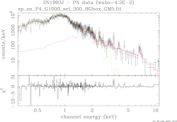
Figure 1: XMM-Newton spectrum as observed with the PN camera and the best fit thermal 2-component model with $kT_{1}$=0.34 keV and $kT_{2}$=6.54 keV. The dashed curves show the low and high temperature component.

Let us first look at the results from the 2-component thermal model fit (2vmekal). The low temperature component of $kT_{1}\sim 0.34\pm 0.04$ keV dominates the spectrum up to energies of about 2 keV, but a higher temperature component is definitely needed to explain the spectrum at higher energies.

Given the fact that the high temperature component takes into account just the band between 3 keV and $\sim$8 keV, where the spectral fit anchors on the Ca IXX, XX and the prominent Fe XXIII, XXIV, XXV line complex, the temperature is likely to be not very well defined. Indeed the temperature of the high temperature component of $kT_{2}\ \sim 6.4\pm{4}$ keV is poorly restricted, because every change in the temperature component is compensated by changes in the abundances of Fe, Ca and Ar. Due to this dependence all the element abundances in the fits have errors typically much larger than the parameter values themselves.Therefore, the abundance values should be considered with some care.

Table 2: Best fit element abundance values from the fit to the PN camera data

el.	2vmekal_T1	2vmekal_T2	2vmekal1	MOS2_T1	vsedov
He	15$\pm 95$	0.1$\pm 273$	0.3$\pm 12$	0.0$\pm 156$	259$\pm 4881$
C	0.0$\pm 172$	-	0.0$\pm 0.1$	0.0$\pm 156$	0.0$\pm$
N	0.0$\pm 172$	-	140$\pm 553$	212$\pm 1908$	6.5$\pm 120$
O	0.15$\pm 1.1$	-	0.2$\pm 0.9$	0.0$\pm 10$	1.1$\pm 20$
Ne	2.0$\pm 11$	0.0$\pm$	2.5$\pm 10$	0.0$\pm 14$	4.0$\pm 75$
Mg	0.4$\pm 2.6$	47$\pm 4531$	0.2$\pm 1.0$	2.0$\pm 16$	6.4$\pm 119$
Al	0.0$\pm$	103$\pm 10000$	0.0$\pm$	13$\pm 104$	-
Si	3.6$\pm 20$	20$\pm 1930$	4.7$\pm 20$	3.7$\pm 30$	7.0$\pm 131$
S	15$\pm 85$	10$\pm 968$	8.4$\pm 35$	8.2$\pm 68$	0.5$\pm 10$
Ar	132$\pm 736$	18$\pm 1777$	16$\pm 68$	0.6$\pm 43$	5.8$\pm$
Ca	95$\pm 541$	3.7$\pm 357$	11$\pm 46$	18$\pm 169$	0.0$\pm 21$
Fe	1.1$\pm 5.9$	1.3$\pm 121$	1.0$\pm 4.0$	1.8$\pm 15$	4.8$\pm 90$

One major difficulty with fitting the vsedov model is based in its enormous demands on computational power. It is therefore difficult to properly scan the parameter space. In the vsedov model the best fit temperatures are somewhat higher than those in the vmekal models. The fit requires additional intrinsic absorption. The lines at higher energies are not very well reproduced by the model.

5 Discussion

How do the X-ray observations fit into the scenario for SN1993J ?

5.1 Earlier X-ray spectra

We have reevaluated the ROSAT data in a homogeneous way Zimmermann97 (Zimmermann et al. 1997) and fitted the spectra with a thermal 1-component model (vmekal in XSPEC) where the element abundances were fixed to either solar or to the values obtained from a similar fit to the XMM-Newton PN spectrum. Due to the high temperatures in the early ROSAT observations there is almost no difference between fitting either solar or XMM-Newton based element abundances. In the November 1993 measurements the fit with the thermal model and solar abundances turned out to be poor but improves significantly (see Tab.  3) with the XMM-Newton based element abundances.

The first ROSAT PSPC spectra do only allow to set a lower limit of $>17$ keV for the temperature of a thermal bremsstrahlung, Raymond & Smith or mekal model. From the ASCA measurements a lower limit of $\ >\,10$ keV was reported. Around the same time the hard X-ray instrument OSSE on the GRO satellite could determine a temperature of $82_{-29}^{+61}$ keV at day 10 to 15 and, statistically already very weak, of $74^{+120}_{-40}$ keV about 1 month after the event Leising94 (Leising et al. 1994). ROSAT measurements half a year later (Zimmermann et al. 1993d, 1994a) revealed a strong decrease from the initial high temperatures to temperatures around 1 keV. An ASCA measurement Uno02 (Uno et al. 2002) confirmed that strong temperature drop.

In terms of the standard 2-shock model it is suggested that the observed emission initially originated from the fast forward shock, while emission from the reverse shock region was blocked at that time by absorbing material due to fast cooling processes in the denser environment. It has been assumed that the initial absorption disappeared on a time scale of the order of 100 days so that half a year later the measured flux was then dominated by the emission from the reverse shock region Zimmermann94 (Zimmermann et al. 1994, Zimmermann et al. 1996, Fransson et al. 1996).

Table 3: ROSAT spectra: best fit parameters of the fit to a 1-component thermal model (vmekal in XSPEC). Abundances were fixed to either solar or to those that resulted from a fit to the XMM-Newton PN spectrum using the same model.

date	kT [keV]	$N_{H}[10^{22}cm^{-2}]$	dof	$\chi 2_{r}$	abund.
April 93	$>$ 17	$0.073^{+0.015}_{-0.012}$	6	0.97	solar
April 93	$>$ 18	$0.071^{+0.005}_{-0.015}$	6	0.96	PN
Nov. 93	$1.60^{+0.2}_{-0.2}$	$0.057^{+0.015}_{-0.015}$	6	2.46	solar
Nov. 93	$1.05^{+0.16}_{-0.13}$	$0.14^{+0.03}_{-0.06}$	6	0.90	PN
April 94	$0.56^{+0.5}_{-0.3}$	$0.70^{+0.07}_{-0.03}$	6	1.05	solar
April 94	$1.05^{+0.16}_{-0.13}$	$0.14^{+0.03}_{-0.06}$	6	0.90	PN

Unfortunately the X-ray lightcurve of SN1993J is not covered between days 50 and 200, so that the transition from the forward shock dominance to the reverse shock remains an open issue.

The Chandra spectrum of May 2000 was fitted by Swartz03 (Swartz et al. 2003) with a 3-component 2vmekal+mekal model. Their best fit model (kT’s of 0.35, 1.01, and 6.0 keV) does not fit the XMM-Newton PN data very well, especially in the energy regime below 0.7 keV, the low and high temperatures are almost identical.

5.2 The X-ray light curve

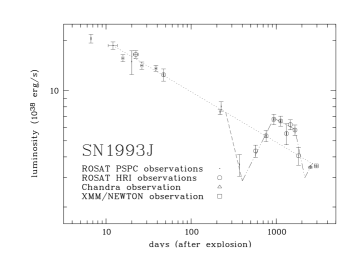
Figure 2: X-ray light curve showing the development of the X-ray luminosity in the 0.3-2.4 keV energy range. The dotted line indicates a decline rate with $t^{-0.30}$. The dashed lines result from model calculations involving time limited decrease and increase of the density in the ambient matter.

The lightcurve in Fig.  2 shows the development of the X-ray luminosity in the energy range 0.3 - 2.4 keV as determined from the 19 ROSAT observations, the Chandra observation from May 2000 and the new XMM-Newton data. The tendency over the first half year is characterized by a decline with $t^{-0.30}$ (Zimmermann et al. 1993c, d), where t is the time since the outburst. Thereafter the lightcurve shows a bump and 5 years after the outburst the luminosity appears to return to the initial decline profile. The CHANDRA observation of 2000 and the XMM-Newton observation in 2001 are very close to the general $t^{-0.30}$ decline.

The mass loss rate of the wind of the progenitor can be expressed as $\dot{M}=4\pi\rho v_{w}r^{s}$, where $v_{w}$ is the wind velocity. For a constant and homogeneous wind $s$ has a value of 2. Under the assumptions that the density $\rho$ of the circumstellar material at radius $r$ is dominated by that wind and the shock velocity stays constant, the observed luminosity is roughly proportional to the square of the density integrated over the emitting volume. In case of a constant and homogeneous wind the luminosity should show a time dependence of $L_{x}\propto t^{-1}$. The flatter time profile $t^{-0.30}$ of the ROSAT luminosity observed during the first half year, corresponds for a spherically symmetric scenario to a density profile with s=1.65. In a more detailed consideration in the framework of the formalism of the standard model the development of the X-ray luminosity produced in the forward shock is expressed by: $L_{x}\ \propto\ T_{e}^{0.16}t^{(3-2s)(n-3)/(n-s)}$ Fransson96 (Fransson et al. 1996), where $r^{-n}$ describes the radial dependence of the density of the SN ejecta. For $n>>10$ it follows $L_{x}\ \propto\ t^{-(2s-3)}$ and taking the observed slow decline with $t^{-0.30}$ the value for $s\ \approx\ 1.65$ is confirmed, in good agreement with results published earlier by Immler01 (Immler et al. 2001).

In the picture of the standard model the shock front, while running outward, is probing increasingly older periods of the progenitor wind with a velocity roughly 1000 times the wind velocity. Thus in 5 years ROSAT scanned about 5000 years of wind history. In our simple formalism the measured time dependence of the luminosity requires that the ratio ’mass loss rate/wind velocity’ decreased during the last 5000 years in the life of the progenitor by more than a factor of 7. This scenario has been investigated in more detail by vandyk94 (Van Dyk 1994) using radio data and by Immler01 (Immler et al. 2001) using the ROSAT data to calculate absolute mass loss rates. The latter authors also speculate that the change of the wind properties might indicate a transition from a red to a blue supergiant phase where mass loss rates are at least an order of magnitude lower and wind velocities may reach 1000 km/s.

The bump in the X-ray light curve suggests a local increase in density above the general power-law profile of the circumstellar matter. It could be attributed to a change in the wind parameters of the progenitor or to an asymmetry caused by a possible binary scenario.

Interesting is a correlation with the expansion velocity of the SN shell that has been derived from high resolution radio images of SN1993J. In Fig. 6 of Bartel02 (Bartel et al. 2002) at about 350 days after the outburst the expansion rate of the radio image size shows a break and continues thereafter at a slower rate. Between day 369 and 1655, the leading edge and the plateau of the bump, the expansion velocity decreases in the order of 28%. The total mass which gave rise to the observed X-ray luminosity bracketing the bump is estimated to $1\ M_{\odot}$. The total mass of the expanding shell covered up to day 350 was of the order of $3\ to\ 4\,M_{\odot}$. Both features, the radio deceleration break and the bump in the ROSAT light curve, independently indicate a flattening of the density profile in the circumstellar medium. Because the break in the expansion curve does not visibly affect the circularity of the radio images one may argue that the cause more likely can be attributed to a density change in the wind instead of an asymmetry by a binary scenario that would possibly affect the circularity of the images.

The closer inspection of the X-ray light curve shows a rapid decline between day 225 and day 370, followed by a rapid increase until day 935. A similar behaviour could have occured between day 1126 and day 1464, but there is just one data point in that period, the upper limit of which is consistent with no change. The rapid decline after day 1655 is very evident and recovery indicated by the Chandra data point at around day 2500 has occured. The existence of the latter two dips is statistically not too convincing, but they may be real as we show below. We suggest that each of the three dips indicates a density depression which is followed by a rise of the density. If the shock wave runs into a sufficiently low density regime no more matter will be shocked and heated, the matter heated so far will simply expand. If the expansion is isothermal the light curve will go down with t^-2; if the expansion is adiabatic the decline will go like t^-8/3, as long as the temperature is higher than about 2 keV. This temperature is about what we would expect at around day 350 (cf. Fig.  3). The falling dashed lines in figure 3 represent such expansion. After some time the shock wave encounters a jump in density to significantly higher values. The density increase raises the emission measure and the X-ray luminosity. Initially the luminosity increases linearly with t when it hits a step like density jump. The rising lines in figure 3 represent such density jumps. The intersection between the rising and falling lines denote the position or epoch of the density jump. We have compared these epochs with those where the highest, discontinuous deceleration of the shock wave has occured, which have been derived from the expansion rate of the radio images (cf. Fig. 6 of Bartel02 (Bartel et al. 2002)). There are also just three such events in the radio images. The two sets of epochs agree surprisingly well with each other to within less than 30 days. We conclude that these changes in the X-ray light curve reflect changes of the density in the ambient matter profile, which appears to show some repetitive pattern. Each of these density increases is preceded by some density decrease like in a wave. Whether this characterizes the activity of the progenitor star as far as the mass loss is concerned remains to be seen.

5.3 Spectral development

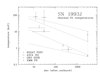
Figure 3: X-ray determined emission temperatures. The dashed lines outline the time evolution of the low and high temperature component using the standard model. For each component there are two lines bracketing the range of the temperatures allowed by the XMM-Newton data using the 2vmekal model.

We can now combine the XMM-Newton temperatures with the ROSAT, ASCA and GRO results. Let us assume for a moment that the initial high temperature, as measured by GRO, originated from the forward shock, while half a year later the flux was dominated by emission from the reverse shock because of the higher electron densities in that region. One can use the similarity solution of the standard model to express in general terms the ratio between the temperatures in the forward and the reverse shocks that depends only on the parameters s and n, $T_{r}/T_{f}\ =\ (3-s)^{2}/(n-3)^{2}$ Fransson96 (Fransson et al. 1996).

With the wind density profile of s=1.65 derived from the light curve, and assuming that the 2 temperatures determined from the thermal 2-component fit to the XMM-Newton spectrum represent the temperatures in the forward and reverse shock regions, we obtain n=8.9 for the density profile of the ejecta. Taking into account the uncertainties of the temperatures as quoted for the PN 2vmekal model, then n results between 6.4 and 10.9.

Entering s and n into the formula that describes the temporal behaviour of the shocks, $T_{r}\propto\ T_{f}\ \propto\ t^{-[2(3-s)/(n-s)]}$ Fransson96 (Fransson et al. 1996), we can extrapolate the XMM-Newton temperatures backward in time and compare them with the ROSAT, ASCA and GRO results (see Fig.  3). The temperature development of the forward shock component is roughly consistent with the temperatures deduced from the GRO data, and also the low temperature development, matching the ROSAT data at day 210, is consistent with its interpretation as coming from the reverse shock region.

But it has to be repeated that, while the parameter s appears reasonably well determined from the light curve (at least for certain periods), the value of n is derived under the assumption of thermal equilibrium between electrons and ions in the emission region. Estimates (see Fransson96 (Fransson et al. 1996)), however, show that even near to the time of the explosion equipartition is not expected in the wind shock.

One can not exclude that we see just emission from the forward shock. The hot material heated in the early days has cooled as it expands, both radiatively and adiabatically with the continuum temperature dropping faster than the higher ionization levels indicate, i.e. we have a delay of the recombination because of the long recombination time scales involved. Thermal equilibrium by just Coulomb collisions and ionization equilibrium is no more reached at times later than about a few days after outburst. Stellar wind matter heated at later stages as the forward shock proceeds is not in thermal equilibrium if not processes other than Coulomb collisions are at work. Therefore the electrons would stay relatively cool and also ionization equilibrium is far from being reached leaving the plasma underionized, which would explain the observation of the low temperature component.

With the sedov model we have tested such a scenario with emission from just one shocked region. But the relatively poor fitting results for the line complexes at higher energies show also that this model is not quite adequate.

6 Conclusions

The XMM-Newton spectrum is well fitted by a thermal 2-component model with ionization equilibrium. The predictions of the standard model describe reasonably well the observed development of the X-ray spectral temperatures, involving both forward and reverse shocks. The equally acceptable fit with a vsedov model shows that at this stage one cannot exclude that only one shock component is at work.

The strong interdependence between the temperature and the values for the abundances of the dominating elements, as far as the high temperature component is concerned, makes it very difficult to interpret the abundance results. But there is clearly no need to involve high values for the metal abundances, which would point to ejecta heated by the reverse shock.

The new XMM-Newton data point in the X-ray lightcurve gives arguments to the assumption of a general decline rate of $L_{x}\propto t^{-0.30}$ and it suggests that the bump in the light curve is probably due to an intermediate density fluctuation. The detailed inspection of the X-ray light curve shows that a density increase did not occur just once, but in some repetitive fashion, There are three dips in the X-ray light curve each one followed by an increase in luminosity. Each of the dips occurred very close to the times when the forward shock velocity underwent a dramatic deceleration as indicated by the expansion rate of the radio images.

The observations show that spatial changes of the powerlaw density profile have no significant impact on the morphology of the radio images, that remain very much circular. This indicates that the bumps in the X-ray lightcurve are more likely caused by density changes in a spherically symmetric wind rather than by asymmetries introduced by a postulated binary companion. For most of the time we need a wind that in the past left more material per volume unit in the circumstellar environment than near to the time of explosion.

References

- (1) Aldering, G., Humphreys, R.M., & Richmond, M. 1994, AJ, 107, 662
- (2) Bartel, N., Bietenholz, M.F., Rupen, M.P., et al. 2002, ApJ, 581, 404-426
- (3) Bartunov, O.S., Blinnikov, S.I., Pavlyuk, N.N., & Tsvetkov, D.Y. 1994, A&A, 281, L53
- (4) Bietenholz, M.F., Bartel, N., & Rupen, M.P. 2001, ApJ, 557, 770-781
- (5) Canizares, C.R., Kriss, G.A., & Feigelson, E.D. 1982, ApJ, 253, L17-L21
- (6) Chevalier, R.A. 1982, ApJ. 259, 302-310
- (7) Fransson, C., Lundqvist, P., & Chevalier, R.A. 1996, ApJ 461, 993-1008
- (8) Freedman, W.L., Hughes, S.M., Madore, et al. 1994, ApJ 427, 628-655
- (9) Immler, S., Aschenbach, B., & Wang, Q.D. 2001, ApJ 561, L107-L110
- (10) Leising, M.D., Kurfess, J.D., Clayton, D.D., et al. 1994, ApJ 431, L95-L98
- (11) Matheson, T., Filippenko, A.V., Ho, L.C., Barth, A.J., & Leonhard, D.C. 2000, ApJ 120, 1499-1515
- (12) Nomoto, K., Susuki, T., Shigeyama, et al. 1993, Nature, 364, 507
- (13) Podsiadlowsky, P.H., Hsu, J.J.L., Joss, P.C., & Ross, R.R. 1993, Nature, 364, 509
- (14) Ray, A., Singh, K.P., & Sutaria, F.K. 1993, Journal of Astrophysics and Astronomy, 14, 53
- (15) Ripero, J., & Garcia, F. 1993. IAU Circ. No. 5731
- (16) Swartz, D.A., Ghosh K.K., McCollough M.L., et al. 2003, ApJS 114, 213-242
- (17) Tanaka, Y. et al. 1993, IAU Circular 5753
- (18) Uno, S., Mitsuda, K., Inoue, H., et al. 2002, ApJ 565, 419-429
- (19) Utrobin, V. 1994, A&A, 281, L89
- (20) Van Dyk, S.D., Weiler, K.W., Sramek, R.A., Rupen, M.P., & Panagia, N. 1994, ApJ, 432, L115-L118
- (21) Woosley, S.E., Eastman, R.G., Weaver, T.A., & Pinto, P.A. 1994, ApJ, 429, 300-318
- (22) Weiler, K.W., Sramek, R.A., Van Dyk, S.D. & Panagia, N. 1993, IAU Circ., 5752, 1
-
(23)
Zimmermann, H.-U., Lewin, W., Magnier, E., et al.
1993a, IAU Circ. No. 5748
1993b, IAU Circ. No. 5750
1993c, IAU Circ. No. 5766
1993d, IAU Circ. No. 5899
1994a, IAU Circ. No. 6014 - (24) Zimmermann, H.-U., Lewin, W., Predehl, P., et al. 1994, Nature, 367, 621
- (25) Zimmermann, H.-U., Lewin, W.H.G., & Aschenbach, B. in Proc. ’Röntgenstrahlung from the Universe’, eds. Zimmermann, H.-U., Trümper, J., & Yorke, H. 1996, MPE Report 263, 289-290
- (26) Zimmermann, H.-U., Becker, W., Belloni, T., et al. 1997, EXSAS User’s Guide, MPE Report 257