Luminosity and Mass Function of the Galactic
open cluster NGC 2422 .

We present UBVRI photometry of the open cluster NGC 2422 (age $\sim\leavevmode\nobreak\ 10^{8}$ yr) down to a limiting magnitude $V\simeq 19$. These data are used to derive the Luminosity and Mass Functions and to study the cluster spatial distribution. By considering the color-magnitude diagram data and adopting a representative cluster main sequence, we obtained a list of candidate cluster members based on a photometric criterion. Using a reference field region and an iterative procedure, a correction for contaminating field stars has been derived in order to obtain the Luminosity and the Mass Functions in the $M=0.4-3.5\leavevmode\nobreak\ M_{\odot}$ range. By fitting the spatial distribution, we infer that a non-negligible number of cluster stars lies outside our investigated region. We have estimated a correction to the Mass Function of the cluster in order to take into account the ”missing” cluster stars. The Present Day Mass Function of NGC 2422 can be represented by a power-law of index $\alpha=3.07\pm 0.08$ (rms) – the Salpeter Mass Function in this notation has index $\alpha=2.35$ – in the mass range $0.9\leq M/M_{\odot}\leq 2.5$. The index $\alpha$ and the total mass of the cluster are very similar to those of the Pleiades.

1 Introduction

Accurate determinations of the stellar Initial Mass Function together with the star formation rate are fundamental to understand star formation mechanisms and related astrophysical problems. Since Salpeter’s estimation of the IMF for stars in the solar-neighborhood (Salpeter, 1955), several investigations in Galactic and extra-galactic stellar systems seem to converge to a universal IMF described by a broken power-law (Scalo, 1998). Many models of stellar population, chemical evolution and galactic evolution adopt a priori a single IMF assuming its universality, although their results are highly sensitive to uncertainties in the IMF (Kennicutt, 1998).

Testing the universality of IMF is a challenge for astrophysicists because several indirect evidences suggest that the IMF ought to systematically vary with the time due to the different star forming conditions (Larson, 1998). Nevertheless, no convincing proofs for a variable IMF still exist and evidences for uniformity of the IMF are deduced by estimates for different populations (Scalo, 1986, 1998; Kroupa, 2002).

However, a large scatter in the logarithmic power-law index, for stars more massive than $1\leavevmode\nobreak\ M_{\odot}$, is evident. In order to understand how large apparent IMF variations are due to uncertainties inherent to any observational estimate of the IMF, Kroupa et al. (2001) investigated the scatter, introduced by Poisson noise and dynamical evolution of star clusters, of the power-law indices inferred for N-body model populations. The resultant apparent variation of the IMF defines a ”fundamental limit” such that any true variation in the IMF that is smaller than this fundamental limit is not detectable. In addition, determinations of the power-law indices are subject to systematic errors arising from unresolved binaries.

Being systems of coeval and equidistant stars with the same chemical composition, open clusters are key samples in investigating the IMF and its possible spatial and temporal variations. Determination of the IMF of open clusters can however be challenging because of the contamination from background Galactic field stars. A further complication comes from the difficulty to transform the observed Present Day Mass Function (PDMF) into the IMF using proper assumptions on the stellar and dynamical evolution, mainly affecting high and low-mass stars, respectively.

In order to reduce these complications it is convenient to study young open clusters or star forming regions. In the low mass star range the IMF is more uncertain but stellar evolution effects are not important; in this mass range the Present Day Mass Function is representative of the IMF.

Additionally, for the question of the universality or variability of the IMF, it is convenient to compare clusters with same age in order to highlight other possible parametric dependence. For these reasons we choose to study the southern Galactic open cluster NGC 2422 which has an age comparable to the well studied Pleiades cluster.

The equatorial (J2000.0) and galactic coordinates of NGC 2422 are RA$=07^{h}36^{m}36^{s}$, Dec=$-$14^∘30^′  (Lynga, 1987), $l$=230^∘.97, $b$=3^∘.13, respectively. Estimates of the fundamental parameters of this cluster, such as age, distance modulus and reddening were given in the past by various authors as summarized by Barbera et al. (2002).

The age of $\sim 10^{8}\leavevmode\nobreak\$yr was estimated using theoretical isochrones (Rojo Arellano et al., 1997); the most recent value of the distance $d=498^{+135}_{-88}$ pc, corresponding to a distance modulus $(M-m)_{0}=8.48^{+0.52}_{-0.42}$, was deduced by Hipparcos measurements on 4 stars (Robichon et al., 1999) while the most recent value of the reddening $E(\hbox{\it B--V\/})=0.088$ was reported by Dambis (1999).

Several papers have been devoted to NGC 2422 in the past: the most recent of them report Strömgren photometry (Shobbrook, 1984; Nissen, 1988; Rojo Arellano et al., 1997), while the available $UBV$ photometric values, either photographic and photoelectric, extend only down to $V\sim 16$ (Zug, 1933; Lynga, 1959; Hoag et al., 1961; Smyth & Nandy, 1962; van Schewick, 1966; Ishmukhamedov, 1967). Mean photometric data and spectral classification from the former papers were compiled by Mermilliod (1986) in a catalog of 212 objects. Using this catalog and 564 additional stars from Ishmukhamedov (1967), Barbera et al. (2002) obtained a large literature-based compilation of measured data of stars in the field of NGC 2422; for some of these stars, X-ray counterparts were found.

The layout of our paper is the following. We present, in Sect. 2, our photometry and astrometry and in Sect. 3 the method adopted to select the candidate cluster member sample. In Sect. 4 we describe how the Luminosity and Mass Functions of NGC 2422 and the spatial distribution of cluster members were obtained. Finally in Sect. 5 we summarize and discuss our results.

2 Cluster UBVRI Photometry and Astrometry

2.1 Observations and Data reduction

The data used in this paper are CCD images in the UBVRI pass-bands collected at the 0.9-m telescope of the Cerro Tololo Inter-American Observatory (CTIO) on January 30, 1997. The scale on the sky of the instrument is 2.028 arcsec/pixel, for a total field of view of $1.15\times 1.15$ square degrees, making such an instrument suitable to cover most of the apparent size of the cluster. The observing log is summarized in Table 1. While the quality of seeing was limited, all images were collected in photometric conditions. Possible effects on the crowded field photometry, due to the limited seeing, have been ruled out by the artificial star test described in Sect. 2.4.

Table 1: Log-book of the NGC 2422 CCD observations

Filter	Exp. Time	Instrumental seeing
	[s]	FWHM[′′]
U	30	3.53
B	15	3.24
V	15	2.70
R	15	2.63
I	23	3.00
I	10	2.99

All the images were pre-processed in a standard way with IRAF, using the sets of bias and sky flat-field images collected during the observing night. The instrumental magnitudes and the positions of the stars for each frame were derived by profile-fitting photometry with the package DAOPHOT II and ALLSTAR (Stetson, 1987). Then we used ALLFRAME (Stetson, 1994) to obtain the simultaneous PSF-fitting photometry of all the individual frames. In order to obtain the transformation equations relating the instrumental magnitudes to the standard UBV (Johnson), $RI$(Kron-Cousins) system, we also derived the instrumental profile-fitting photometry for the two Landolt (1992) fields of standard stars SA95 and SA98 observed during the same night.

In order to obtain the total integrated instrumental magnitudes we derived aperture photometry for the same stars that we used to define the PSF, after the digital subtraction of neighboring objects from the frames. We used DAOGROW (Stetson, 1990) to obtain the aperture growth curves for each frame and to compute the aperture correction to the profile-fitting photometry.

The transformation coefficients to the standard system were derived using transformation equations of the form:

$$v =V+A_{0}+A_{1}\times X+A_{2}\times(\hbox{\it V--I\/}),$$

$$b =B+B_{0}+B_{1}\times X+B_{2}\times(\hbox{\it B--V\/}),$$

$$i =I+C_{0}+C_{1}\times X+C_{2}\times(\hbox{\it V--I\/}),$$ (1)

$$r =R+D_{0}+D_{1}\times X+D_{2}\times(\hbox{\it V--R\/}),$$

$$u =U+E_{0}+E_{1}\times X+E_{2}\times(\hbox{\it U--B\/}).$$

Table 2: Coefficients of the calibration equations.

$A_{0}$	$A_{1}$	$A_{2}$
$4.637\pm 0.009$	$0.14$	$-0.012\pm 0.010$
$B_{0}$	$B_{1}$	$B_{2}$
$5.574\pm 0.002$	$0.25$	$0.095\pm 0.005$
$C_{0}$	$C_{1}$	$C_{2}$
$5.100\pm 0.002$	$0.05$	$-0.008\pm 0.002$
$D_{0}$	$D_{1}$	$D_{2}$
$4.352\pm 0.007$	$0.10$	$-0.029\pm 0.012$
$E_{0}$	$E_{1}$	$E_{2}$
$6.989\pm 0.002$	$0.55$	$-0.048\pm 0.008$

In these equations $v$, $b$, $i$, $r$ and $u$ are the aperture magnitudes, already normalized to 1 sec exposure and $X$ is the airmass.

Due to the limited number of standard star observations, we do not have a complete coverage of airmass and we have not been able to derive the extinction coefficients. In order to overcome this problem, we used typical values for CTIO available at http://www.noao.edu/scope/ccdtime/ctio.db; both the adopted extinction coefficients and the best fit values for the zero points and the color coefficients are summarized in Table 2. Second order color terms were tried and turned out to be negligible in comparison to their uncertainties.

The calibration process we have adopted is based on two sequential steps, following a procedure adopted by Stetson (private communication). First, 45 program stars on the NGC 2422 images were selected using the condition (following a criterion described in Stetson, 1993, Sect. 4.1) that each star has to be well separated from its neighbors, observed in all frames, and with a statistic index $\chi$, relative to the goodness of the PSF-fitting photometry, less than 1.5. The photometric calibration based on the Landolt standards is applied to these selected stars only (which we refer to as local standards), which were then used (together with the Landolt standard stars) to calibrate the other program stars.

2.2 Astrometry

The astrometric solution has been computed using as reference the recently released Guide Star catalog, Version 2.2.01 (GSC 2.2). At beginning, our pixel coordinate list was matched to the celestial coordinate list of the GSC 2.2 by projecting the celestial coordinates onto a plane and using as reference three stars for which we had both the pixel and the celestial coordinates from the Hipparcos catalog (Turon et al., 1993).

An initial estimate for the linear transformation has been computed using the reference coordinates of the 1350 matched stars. Then, a plate solution has been computed using the same matched pixel and celestial coordinates by fitting a power series polynomial (IRAF task CCMAP). The final accuracy is of 0.24 arcsec. Finally, the IRAF tasks CCSETWCS and SKYPIX were used to obtain the celestial coordinates of the total sample.

2.3 The Color-Magnitude Diagram

In order to obtain the color-magnitude diagram (CMD) of the cluster, a selection based on the sharp parameter was first done following Stetson (1987). The sharp parameter is related to the angular size of the astronomical object allowing to reject non-stellar objects as semi-resolved galaxies and unrecognized blended double stars, for which sharp is significantly greater than zero, or cosmic rays, for which sharp is significantly less than zero. We considered stellar objects those having the sharp parameter in the $(-0.2\leavevmode\nobreak\ -\leavevmode\nobreak\ +0.2)$ range. In this way we obtained a list of 36 101 stellar objects for which we have $V$ and $I$ magnitudes. For 35 732 of these we have VRI magnitudes, for 35 140 we have BVRI magnitudes and finally, for 33 494 we have UBVRI magnitudes.

The $V$ vs. V–I  color-magnitude diagram  for all the stellar objects in the NGC 2422 field is shown in Fig. 1 (left upper panel). Horizontal bars indicate the median errors in color, while vertical bars indicate the median errors in magnitude for bins of one magnitude. Clearly, the diagram is heavily contaminated by background and foreground stars, as expected from the position of the cluster in the Galactic disk.

In order to determine the cluster main sequence minimizing the contamination effects, we show in Fig. 1 (right upper panel) the $V$ vs. V–I  color-magnitude diagram  approximately corresponding to the cluster core. The centroid of this circular region of $\simeq 16$ arcmin of radius has been estimated using the stars with $V\leq 11.5$.

We considered several theoretical isochrones available in literature (Siess et al., 2000; Baraffe et al., 1998; Girardi et al., 2000; Castellani et al., 1999) and we have found that the cluster main sequence is well fitted by the 100 Myr and solar metallicity (Z = 0.02) theoretical isochrone computed by Siess et al. (2000, SDF00), for higher mass stars ($M>0.6M_{\odot}$), and the one computed by Baraffe et al. (1998, BCAH98) with a general mixing length parameter $\alpha=1$, for lower mass stars ($M<0.6M_{\odot}$). Both isochrones were transformed into the $V$ vs. V–I  plane using the apparent distance modulus $(m-M)_{V}=8.76$, derived from the distance modulus $(m-M)_{0}=8.48$ of Robichon et al. (1999) and the interstellar absorption $A_{V}=0.273$, from the standard relation $R_{V}=A_{V}/E(\hbox{\it B--V\/})=3.1$ (Mathis, 1990) where the reddening $E(\hbox{\it B--V\/})=0.088$ is the value calculated by Dambis (1999). The color excesses $E(\hbox{\it V--I\/})=0.11$, $E(\hbox{\it R--I\/})=0.06$, $E(\hbox{\it U--B\/})=0.07$ were derived using the relations for $R_{V}=3.1$ given by Munari & Carraro (1996). As shown in Fig. 1 (left lower panel), the resulting theoretical isochrone is in good agreement with the apparent cluster main sequence, confirming the literature cluster parameters, such as distance and reddening.

Furthermore, using a set of theoretical isochrones by Siess et al. (2000) for different ages, and the well defined main sequence of bright stars in the $B$ vs. U–B  color-magnitude diagram, we verified that the NGC 2422 age is $\simeq 10^{8}$ yr, in agreement with the value given by Rojo Arellano et al. (1997).

Finally, we matched our photometric data with the X-ray sources of Barbera et al. (2002). The matched stars are plotted with large squares in Fig. 1 (right lower panel). There are two populations of X-ray sources: a blue faint population, dominated by background objects, and a group of sources belonging to the cluster main sequence. The photometric position of the X-ray members allow us to confirm our choice of the main sequence.

In Fig. 2, we show the $V$ vs. V–I, $I$ vs. R–I, $V$ vs. B–V and $B$ vs. U–B  color-magnitude diagrams  for the stars in the NGC 2422 field. The curve in the $V$ vs. V–I  and in the $I$ vs. R–I  color-magnitude diagrams  is the Siess et al. (2000) theoretical isochrone extended to lower stars using the Baraffe et al. (1998) theoretical isochrone as described above. For the other two diagrams we only considered stars with $\sigma_{B}<0.03$ and $\sigma_{U}<0.03$, respectively, and the Siess et al. (2000) theoretical isochrone because we use the $V$ vs. B–V  and the $B$ vs. U–B  color-magnitude diagrams  to select only the bright cluster members.

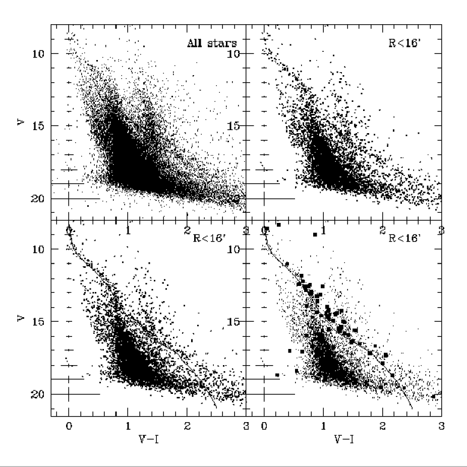
Figure 1: The $V$ vs. V–I  color-magnitude diagram  for the full catalog (left upper panel) and for stars within $\sim 16$ arcmin from the centroid (right upper panel and lower panels). The curve is the adopted theoretical isochrone (see text) and the large squares indicate the positions of the stars which have X-ray counterparts in Barbera et al. (2002). Horizontal bars indicate the median errors in color, while vertical bars indicate the median errors in magnitude for bins of one magnitude.

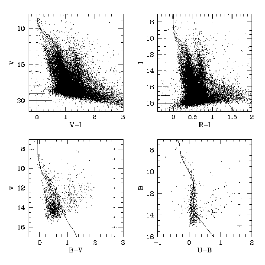
Figure 2: The $V$ vs. V–I, $I$ vs. R–I, $V$ vs. B–V  and $B$ vs. U–B  color-magnitude diagrams for the stars in the NGC 2422 field. Horizontal bars indicate the median errors in color, while vertical bars indicate the median errors in magnitude for bins of one magnitude. The solid lines are the theoretical isochrones described in the text. In the $V$ vs. B–V  and $B$ vs. U–B  color-magnitude diagrams only stars with $\sigma_{B}<0.03$ and $\sigma_{U}<0.03$, respectively, are indicated.

2.4 Data completeness and photometric errors

Since we are interested in deriving the Luminosity Function from star counts and because of the limited seeing of our data, particular attention has been devoted to estimate the accuracy of the photometry and the completeness of the derived star list. For this, a list of artificial stars was created and added to the original frames in order to compare the photometric results of the recovered artificial stars and the input values.

In order to avoid overcrowding, the artificial stars were placed in a spatial grid (cf. Piotto & Zoccali, 1999) such that the separation of the centers in each star pair was four PSF radii plus 1 pixel. Using a random-number generator for the $V$ magnitudes, a list of 2470 stars ($7\%$ of the total sample) with a flat distribution of the instrumental $V$ magnitudes between 11 and 21.5 was created. These limits were chosen on the basis of the instrumental $V$ vs. V–I  color-magnitude diagram. The $V$ magnitudes for each artificial star were converted to the other filters using the fiducial lines representing the $V$ vs. V–I, $V$ vs. B–V, $I$ vs. R–I  and $B$ vs. U–B  color-magnitude diagrams.

DAOPHOT’s ADDSTAR routine was used to add these artificial stars into copies of the original data frames, with the appropriate frame-to-frame shifts in their position and brightness. Calibrated magnitudes were derived using the same photometric parameters and the same procedure described in Sect. 2.1.

We estimated the completeness fraction as the ratio between the number of artificial stars recovered simultaneously in the $V$, $I$ and $R$ filters and the number of added stars per one magnitude bin. This condition was imposed because the photometric selection of low-mass candidate cluster members was based on the use of $V$ vs. V–I  and $I$ vs. R–I  color-magnitude diagrams.

We found that this ratio is equal to 1 down to $V=18.26$, while it decreases to $0.94\pm 0.06$ to the limit $V\simeq 19$ of our data. Therefore, we can conclude that our catalog is complete down to $V=18.26$ over the whole $V$ vs. V–I  and $I$ vs. R–I  color-magnitude diagrams  while it is $94\%$ complete to $V=19$, so that a $\sim 6\%$ correction will be required to the number of faintest stars when computing the Luminosity Function.

Finally, photometric errors were estimated by the differences between the ”observed” magnitudes and colors derived for the artificial stars and their known input values. We defined the external error $\hat{\sigma}_{\rm ext}$ for the $V$ magnitudes and for the V–I  and R–I  colors as in Stetson & Harris (1988); the results are summarized in Table 3.

Table 3: External photometric errors from the artificial star photometry.

$\Delta V$	$\hat{\sigma}_{{\rm ext},V}$	$\hat{\sigma}_{{\rm ext},V-I}$	$\hat{\sigma}_{{\rm ext},R-I}$
9.5  - 10.5	0.001	0.001	0.001
10.5 - 11.5	0.001	0.003	0.003
11.5 - 12.5	0.003	0.004	0.003
12.5 - 13.5	0.006	0.006	0.004
13.5 - 14.5	0.007	0.009	0.007
14.5 - 15.5	0.013	0.016	0.010
15.5 - 16.5	0.024	0.025	0.018
16.5 - 17.5	0.043	0.058	0.039
17.5 - 18.5	0.111	0.105	0.080
18.5 - 19.5	0.225	0.248	0.098

3 Photometric selection of Candidate Cluster Members

In order to select possible NGC 2422 cluster members, we used only photometric informations as described in the following steps:

1. In the $V$ vs. V–I  color-magnitude diagram, we selected as possible candidate members all those stars which, according to their $\sigma_{V}$ and $\sigma_{V-I}$ errors, belong to a well defined strip in the CMD. The lower envelope of this strip follows the representative main sequence for the cluster (see Sect. 2.3) while the upper envelope is displaced upward by 1 mag to include binaries. We have choosen 1 mag instead of the canonical 0.75 mag since our isochrone is, in some points of the diagram, slightly lower than the apparent ”true” sequence of the cluster (see Fig. 1). With our larger strip we are sure to include X-ray detected stars that are probable members since significant X-ray emission is a common property of young stars. After this selection, our sample contains 2059 possible candidate members.

2. We considered at first only those stars (1895) for which UBVRI  photometry was available. We constructed an analogous strip as above, in the $I$ vs. R–I  color-magnitude diagram  and we rejected from our sample of initial possible candidate members 540 stars which, according to their $\sigma_{I}$ and $\sigma_{R-I}$ errors, do not belong to the strip in the $I$ vs. R–I  color-magnitude diagram.

3. From the resulting sample, we considered only the 333 stars having typical error in $B$ magnitude less than 0.03. We saw that this occurs for $B\leq 16$. Therefore, using the Siess et al. (2000) isochrone, we constructed in the $V$ vs. B–V  color-magnitude diagram  an analogous strip and we rejected those 58 stars that, according to their $\sigma_{V}$ and $\sigma_{B-V}$ errors, do not belong to the strip.

4. Subsequently, we allowed for the $B$ vs. U–B  color-magnitude diagram  to select the bright stars with $U\leq 13.5$ for which the errors in U magnitude are less than 0.03 mag. Using the same criterion as above, we defined a strip taking into account the isochrone’s shape in this diagram thus further rejecting 195 stars.

5. Finally, we considered the stars for which only VRI magnitudes are available. As above, we considered as possible cluster candidate members those belonging to the strip defined in the $I$ vs. R–I  color-magnitude diagram.

In our final sample we retained only those stars with $\sigma_{I}\leq 0.3$ mag.

The selection procedure described above was chosen to take advantage of all the available photometric informations and to avoid excluding too many possible cluster members.

The photometric/astrometric catalog of the candidate cluster members, containing 1277 stars, is given in Table 4 where we report RA and Dec (J2000.0) coordinates in decimal degrees, an identification number for each star, the $U,\leavevmode\nobreak\ B,\leavevmode\nobreak\ V,\leavevmode\nobreak\ R,\leavevmode\nobreak\ I$ magnitudes and the associated uncertainties.

Fig. 3 shows these cluster candidates in the color-magnitude diagrams  so far considered. Clearly, the sample includes contaminating objects that do not belong to the cluster. The approach to estimate and to deal with such a contamination will be described in the following section.

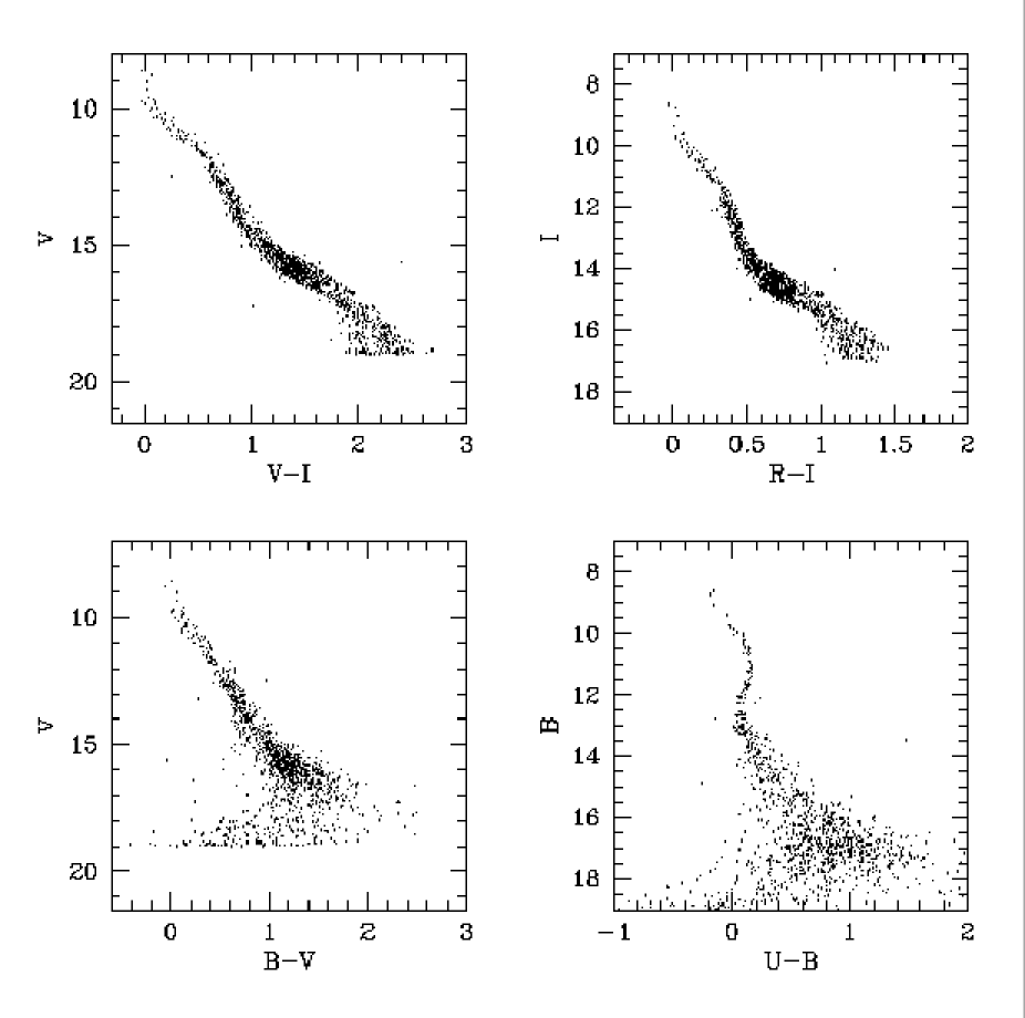
Figure 3: The color-magnitude diagrams  for the possible photometric candidate members of NGC 2422. The sample has been obtained as described in Sect. 3.

4 Determination of Luminosity and Mass Functions and Spatial Distribution

To construct the Luminosity and Mass Functions of the cluster we need to correct the luminosity distribution of our selected sample for field star contamination. To quantify the contamination we adopted an iterative procedure schematically summarized in the following steps:

1. We defined as “field region” an area of our field of view where we expect to find only few cluster stars. We used such a region to quantify the field star contribution and then to obtain a first approximation of the cluster Luminosity and Mass Functions as well as of the cluster spatial distribution from stellar counts in a circular area centered on the cluster centroid.

2. By fitting King’s empirical profiles (King, 1962) to the cluster spatial distribution we then estimated the total number of cluster members beyond our cluster region and the number of cluster members contaminating the “field region”.

3. After correcting the field star luminosity distribution and the field star spatial distribution for cluster stars falling in the field region, we re-obtained the cluster Luminosity and Mass Functions and the cluster spatial distribution. By re-fitting King’s empirical profiles to the new cluster spatial distribution we re-estimated the total number of cluster members beyond our field of view in order to correct the cluster Mass Function.

4. We re-corrected the field star luminosity distribution and we repeated the above step 3. The entire procedure was rapidly convergent and indeed the “step 3” correction was applied only three times, since after the third application the previous and final corrected Mass Function differ by less than $1\%$, i.e. well within the intrinsic uncertainties.

4.1 First approximation of Luminosity and Mass Functions

As summarized above, a first approximation to the contamination of foreground and background sources has been obtained using the lower region of our field where we expect to find only few cluster stars. In fact, as shown in Fig. 4, the cluster is mainly concentrated in the upper region of our field where we defined the ”central cluster region” corresponding to the circular area within the radius of $27.07$ arcmin. A value for the cluster centroid position has been calculated as the median value of the $X$ and $Y$ coordinates of the bright stars ($V\leq 12$). This position corresponds to the equatorial coordinates (J2000.0) $RA=7^{h}36^{m}34^{s}.8,Dec=-14^{\circ}29^{\prime}18^{\prime\prime}.5$. We verified that the coordinates of the centroid do not change significantly if the $V$ magnitude limit changes in the $11.5\leq V\leq 13$ range.

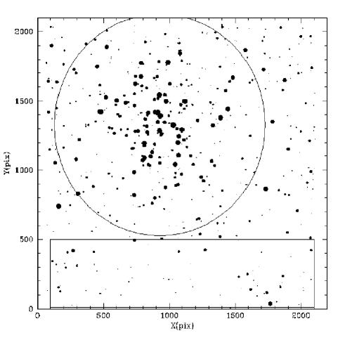
Figure 4: A map of the brightest selected stars in the total field of view ($1.15\times 1.15$ square degrees). Biggest dots represent stars with $V\leq 9$ while smallest dots represent stars with $15.3\leq V\leq 15.7$. The circle delimits the area chosen to estimate the Luminosity Function of the cluster, while the rectangle delimits the area chosen to estimate the contamination rate of foreground and background stars.

We consider the rectangular region in Fig. 4, of $67.6\times 13.52\leavevmode\nobreak\ {\rm arcmin}^{2}$ size ($2000\times 400\leavevmode\nobreak\ {\rm pixels}$), as representative of the Galactic field (the ”field region”), i.e. we suppose that the observed luminosity distribution in the rectangular region is given by

$$\hat{N}_{\rm f}(V)=\hat{N}_{{\rm f},0}(V)+\hat{N}_{\rm cl}(V)\simeq\hat{N}_{{\rm f},0}(V),$$ (2)

where $\hat{N}_{{\rm f},0}(V)$ is the ”true” field star luminosity distribution, while $\hat{N}_{\rm cl}(V)$ is the cluster star contribution within the rectangular region. Therefore, the field star luminosity distribution in the ”central cluster region” is given by

$$N_{\rm f}(V)=\hat{N}_{\rm f}(V)\frac{A}{\hat{A}},$$ (3)

where $A$ and $\hat{A}$ are the area of the ”central cluster region” and of the ”field region”, respectively.

The NGC 2422 Luminosity Function, $N_{\rm cl}(V)$, has hence been obtained subtracting the field star luminosity distribution, $N_{\rm f}(V)$, from the luminosity distribution of all the stars in our sample within the ”central cluster region”, $N_{\rm t}(V)$. Fig. 5 shows the contaminated luminosity distribution of the candidate members (dotted line), the luminosity distribution of the field stars (dashed line) and the Luminosity Function of NGC 2422 obtained as described above and corrected for incompleteness as derived in Sect. 2.4 (solid line). We found that the contamination rate from field stars is negligible for the brightest stars, but starts to become significant at $V\simeq 13$ where it is of the order of the $40\%$. At fainter magnitudes this value increases with a peak of the order of $\sim 90\%$ around $V\simeq 16$ where the contribution of the field giant stars is dominant. The total number of the cluster members estimated at this step is 347.

Figure 5: Luminosity distribution of the candidate members without correction for contamination (dotted line), the luminosity distribution of the field stars (dashed line) and the Luminosity Function of NGC 2422 (solid line) obtained as difference between the last two and corrected for incompleteness, as described in Sect. 2.4.

The Luminosity Function obtained at this step has been transformed into a first approximation of the Mass Function, $\xi^{0}(M)$, using the mass-visual magnitude relation derived from the same models that we used to fit the cluster color-magnitude diagrams. The resultant first approximation of the Present Day Mass Function, extending from $0.5$ to $3.5\leavevmode\nobreak\ M_{\odot}$, is shown in Fig. 6.

As already mentioned, due to dynamical evolution, the angular size of the cluster is almost certainly larger than the investigated ”central cluster region” hence this Mass Function is not representative of the whole cluster mass distribution. In order to estimate the correction to the Mass Function due to the dynamical evolution, we studied the spatial distribution of NGC 2422 as described in the following Sections.

Figure 6: First approximation of the NGC 2422 Present Day Mass Function obtained in our central cluster region and without any correction. $\xi^{0}(M)$ values are given in number per logarithmic mass unit.

4.2 First approximation of the Spatial Distribution

The spatial distribution of the cluster members was studied in order to investigate the cluster dynamical evolution and to determine the cluster dynamical parameters. As first approximation, we corrected the radial surface density distribution of candidate cluster members for foreground and background contaminating stars assuming that the field stars are uniformly distributed, i.e.

$$\frac{dN}{dr}=2\rho\pi r,$$ (4)

where $r$ is the distance from the cluster center and $\rho$ is the star distribution for unit of area in the rectangular region considered in Sect. 4.1.

In order to take into account the dynamical evolution and mass segregation effects due to the energy equipartition (see Kroupa et al., 2001 and relative references), we subdivided the stars into 4 bins of $V$ magnitude as in Table 5. In Fig. 7 we present the cluster surface density profiles in ${\rm stars/arcmin}^{2}$ as a function of radius in parsec, assuming the distance value of $497.5$ pc by Robichon et al. (1999).

Figure 7: The radial distribution of stellar density in NGC 2422, for 4 different bins of magnitude.

We fitted King’s empirical profiles (King, 1962), given by

$$\rho(r)=\rho_{0}(\frac{1}{\sqrt{1+(r/r_{\rm c})^{2}}}-\frac{1}{\sqrt{1+(r_{\rm t}/r_{\rm c})^{2}}})^{2},$$ (5)

to the surface density profiles. In this equation, $\rho_{0}$ is a normalization constant, $r_{\rm c}$ is the ”core radius” determined by the internal energy of the system and $r_{\rm t}$ is the tidal radius where the cluster disappears.

The tidal radius was calculated as in Jeffries et al. (2001) as $r_{\rm t}=1.46\leavevmode\nobreak\ M_{\rm c}^{1/3}$, where $M_{\rm c}$ is the cluster mass in solar masses. In order to estimate the total mass of the cluster we integrated the Mass Function obtained in Sect. 4.1 and found a value of $M_{\rm c}=357\pm 35\leavevmode\nobreak\ M_{\odot}$, corresponding to the tidal radius value $r_{\rm t}=10.36\pm 0.34$ pc.

The results of King’s empirical profile fitting, with the 1-$\sigma$ uncertainty estimates for the parameters, are reported in Table 5 and are shown in Fig. 7. Comparing the $\chi^{2}$ values with the number of degrees of freedom ($\nu=6$), we conclude that the fits are all acceptable.

Table 5: Results of King’s empirical profile fitting to the radial surface density distribution. Columns 1 and 2 give the $V$ magnitude ranges and the corresponding mass ranges; Col. 3 the fitted normalization constant, Col. 4 the assumed tidal radius, Col. 5 the fitted core radius, Col. 6 the $\chi^{2}$ of the fitting. Finally, Col. 7 lists the number of counted cluster members in our investigated region for each magnitude subset, while Col. 8 and 9 are the total number of cluster members predicted by the fitted model within the investigated radius ($\sim 3.7$ parsec) and the tidal radius, respectively. The values are given for each of the four step of the adopted iterative procedure.

$\Delta V$	$M$	$\rho_{0}$	$r_{\rm t}$	$r_{\rm c}$	$\chi^{2}$	$N_{\rm sur}^{\rm cl}$	$N_{\rm sur}^{\rm cal}$	$N_{\rm tid}$
	$(M_{\odot})$	$({\rm stars/arcmin}^{2})$	(pc)	(pc)
			ITERATION 0
8.50 - 11.13	3.7 - 1.7	$0.21\pm 0.10$	$10.36$	$0.59\pm 0.22$	4.2	34	29	33
11.13 - 13.75	1.7 - 1.0	$0.22\pm 0.13$	$10.36$	$1.34\pm 0.46$	8.5	88	76	95
13.75 - 16.38	1.0 - 0.7	$0.27\pm 0.24$	$10.36$	$1.49\pm 0.73$	1.3	106	101	129
16.38 - 19.00	0.7 - 0.4	$0.22\pm 0.26$	$10.36$	$2.66\pm 1.48$	2.5	119	111	164
			ITERATION 1
8.50 - 11.13	3.7 - 1.7	$0.21\pm 0.10$	$10.57$	$0.62\pm 0.23$	4.0	35	30	34
11.13 - 13.75	1.7 - 1.0	$0.23\pm 0.13$	$10.57$	$1.36\pm 0.44$	8.7	93	81	103
13.75 - 16.38	1.0 - 0.7	$0.27\pm 0.24$	$10.57$	$1.55\pm 0.74$	1.3	113	108	140
16.38 - 19.00	0.7 - 0.4	$0.24\pm 0.25$	$10.57$	$2.65\pm 1.30$	2.5	134	124	185
			ITERATION 2
8.50 - 11.13	3.7 - 1.7	$0.21\pm 0.10$	$10.60$	$0.62\pm 0.23$	3.9	35	30	35
11.13 - 13.75	1.7 - 1.0	$0.22\pm 0.12$	$10.60$	$1.40\pm 0.45$	8.7	94	80	102
13.75 - 16.38	1.0 - 0.7	$0.27\pm 0.24$	$10.60$	$1.58\pm 0.76$	1.3	115	109	142
16.38 - 19.00	0.7 - 0.4	$0.24\pm 0.26$	$10.60$	$2.78\pm 1.41$	2.4	136	125	191
			ITERATION 3
8.50 - 11.13	3.7 - 1.7	$0.21\pm 0.10$	$10.61$	$0.62\pm 0.23$	3.9	35	30	35
11.13 - 13.75	1.7 - 1.0	$0.22\pm 0.12$	$10.61$	$1.39\pm 0.47$	8.7	94	80	102
13.75 - 16.38	1.0 - 0.7	$0.27\pm 0.24$	$10.61$	$1.58\pm 0.75$	1.3	115	109	142
16.38 - 19.00	0.7 - 0.4	$0.24\pm 0.27$	$10.61$	$2.86\pm 1.47$	2.4	137	127	195

From the resulting distribution we can see that, while the distribution of the brightest stars vanishes to zero as the radius increases (at the top on the left of Fig. 7), the other profiles tend to non negligible values when fainter $V$ magnitudes are considered. This result suggests an evidence of mass segregation of high mass cluster stars toward the center of the cluster and low mass cluster stars out of our investigation region of $27$ arcmin of radius. This conclusion is confirmed by the increase of the core radius as the mass decreases.

In order to estimate the fraction of low-mass stars beyond the ”central cluster region”, we extrapolated the surface density profiles as far as the tidal radius. Using the integral of equation 5 as given by King (1962), we calculated, for each bin of magnitude, the total number of cluster stars within the tidal radius, indicated in Table 5 by $N_{\rm tid}$. We compared the calculated total number $N_{\rm tid}$ with the number of cluster members $N_{\rm sur}^{\rm cl}$, detected in our survey, that is within $r_{\rm sur}=3.7$ pc and we found that while the stars with $V\lesssim 11$ are all in the investigated region, the fraction of the cluster stars lying outside our survey is $8\%$ for $11.13\leq V\leq 13.75$, $22\%$ for $13.75\leq V\leq 16.38$ and $38\%$ for $16.38\leq V\leq 19.00$. In order to verify the consistency of these numbers we also integrated King’s empirical profile within the radius $r_{\rm sur}$, indicated by $N_{\rm sur}^{\rm cal}$, finding consistent values with the number of the cluster stars found in the central cluster region ($N_{\rm sur}^{\rm cl}$).

The results of the King’s empirical profile integration also suggest that the cluster star contribution within the adopted ”field region”, $\hat{N}_{\rm cl}(V)$ is non-negligible and that the estimated field star luminosity and spatial distributions have to be corrected for the cluster star contamination. In order to estimate the correction factor, we split the ”field region” in a grid of $5\times 20$ subregions and we calculated the King’s profile surface density, $\rho(r_{i})$, where $r_{i}$ is the radius of the centers of each subregion $i$. Therefore, the total number of cluster stars within the ”field region”, per magnitude bin, is given by

$$\hat{N}_{\rm cl}(V)=A_{\rm s}\sum_{i}{\rho(r_{i})},$$ (6)

where $A_{\rm s}$ is the area of each subregion.

Finally, using equation (2), we estimated a more accurate field star distribution as

$$\hat{N}_{{\rm f},0}(V)=\hat{N}_{\rm f}(V)-A_{\rm s}\sum_{i}{\rho(r_{i}).}$$ (7)

4.3 Luminosity and Mass Functions

Using the value of $\hat{N}_{{\rm f},0}(V)$ from Eq. (7) and the iterative approach described in Sect. 4, we recomputed the Luminosity Function of the cluster taking into account the presence of cluster stars in the “field region”.

This final Luminosity Function has been converted into a Mass Function that has been integrated to compute a new value for the total mass ($M_{\rm c}\simeq 385\leavevmode\nobreak\ M_{\odot}$), corresponding to $r_{\rm t}\simeq 10.61$ pc. Dynamical parameters were also obtained in the various iterations, and by integration of King’s profiles we interpolated the ratio $R=N_{\rm sur}^{\rm cl}/N_{\rm tid}$, deriving a factor $1/R$ for the Mass Function to correct for the cluster stars lying beyond the investigated cluster region. The corrected Mass Function has been computed by the expression:

$$\xi^{1}_{c}(M)=\xi^{1}(M)/R.$$ (8)

In Fig. 8 we compare the final Mass Function, $\xi_{c}(M)$, with the Mass Function derived from the central cluster region but without correction for dynamical evolution. We also compare them with the Pleiades Mass Function derived using the Lee & Sung (1995) Luminosity Function and the same mass-luminosity relation used for NGC 2422 in the present work.

Figure 8: Comparison of the NGC 2422 Mass Function corrected for dynamical evolution effects (filled points) with the NGC 2422 Mass Function without correction for dynamical evolution (empty triangles) and with the Pleiades one (empty circles). The line is the power law fitting the MF in the $0.9\leavevmode\nobreak\ -\leavevmode\nobreak\ 2.5\leavevmode\nobreak\ M_{\odot}$ range. $\xi(M)$ values are given in number per logarithmic mass unit.

According to the recently proposed analytical IMF forms (Kroupa, 2002), we considered a multi-part power-law IMF to fit our data. We found that in the mass range $0.9\leq M/M_{\odot}\leq 2.5$ the value of $\alpha$ is $3.09\pm 0.09$ (rms) and $2.63\pm 0.16$ for NGC 2422 and Pleiades, respectively. The latest value is very close to the value 2.67 derived by Barrado y Navascués et al. (2001) for the Pleiades, using the Hambly et al. (1999) data in the $0.6\leavevmode\nobreak\ -\leavevmode\nobreak\ 10\leavevmode\nobreak\ M_{\odot}$ mass range. The two values here derived are in better agreement, within the errors, with the Scalo (1998) value $\alpha=2.7\pm 0.3$ rather than with the Salpeter (1955) value $\alpha=2.35$.

Using the final Mass Function, we also estimated the corrected cluster total mass ($M_{\rm c,cor}\simeq 453\leavevmode\nobreak\ M_{\odot}$) and we compared this value with the NGC 2422 total mass estimated within the ”central cluster region”, $M_{\rm c}\simeq 385\leavevmode\nobreak\ M_{\odot}$. In the same mass range ($0.5\leavevmode\nobreak\ -\leavevmode\nobreak\ 3.5\leavevmode\nobreak\ M_{\odot}$), the total mass of the Pleiades is $M_{\rm Pl}=467\pm 26\leavevmode\nobreak\ M_{\odot}$, a value very similar to the one of NGC 2422. We note that our estimate of the total mass of NGC 2422 is, in any case, a lower limit, since we do not have taken into account the presence of companions in photometric binaries.

5 Summary and Conclusions

Using UBVRI images, covering a field of view of $1.15\times 1.15$ square degrees, we extracted a photometric and astrometric catalog of the stars in the field of NGC 2422 down to $V\simeq 19$ ($M\simeq 0.4\leavevmode\nobreak\ M_{\odot}$). Adopting a representative cluster main sequence to the color-magnitude diagrams, a photometric criterion was defined to obtain a list of candidate cluster members. A test with artificial stars allowed us to verify that our data are complete down to $V=18.26$ while a correction of $\simeq 6\%$ was necessary for the lowest $V$ range ($18.26\leq V\leq 19.26$) in deriving the Luminosity Function.

We have defined a ”central cluster region” within a radius of $27.07$ arcmin from the cluster centroid and a ”field region” of $1.12\times 0.23$ square degrees to estimate the contamination of background and foreground stars. An initial determination of the Luminosity and Mass Functions has been obtained assuming that all the cluster stars lie in the ”central cluster region”. By applying an iterative procedure we have estimated the number of cluster stars within the ”field region” in order to obtain a more accurate correction of the cluster Luminosity Function for field star contamination.

Evidence for mass segregation and energy equipartition have been found from the spatial distribution of the stars. Extrapolation of the King (1962) empirical model allows us to infer that, while all the stars with $M\geq 1.7\leavevmode\nobreak\ M_{\odot}$ are inside the ”central cluster region”, a non negligible fraction of lower mass stars lies outside. In particular, by integrating the spatial distribution within the tidal radius we are able to estimate the number of cluster stars lying beyond the ”central cluster region” and within the tidal radius. Therefore, we are able to estimate a correction to the Mass Function in order to take into account the cluster dynamical evolution.

The corrected Present Day Mass Function was compared with that of the Pleiades which is known down to the brown dwarf limit ($0.08\leavevmode\nobreak\ M_{\odot}$). We found that, in the mass range $0.9\leq M/M_{\odot}\leq 2.5$, the Mass Function of NGC 2422 can be represented by a power law of index $\alpha=3.09\pm 0.08$ (rms) comparable with the index $\alpha=2.63\pm 0.15$ obtained for the Pleiades in the same mass range. The index is also consistent with the data presented in the log $M$ vs. $\alpha$ plot of Kroupa (2002).

By taking into account the correction due to the dynamical evolution, we computed a lower limit of the total mass of NGC 2422 as $M_{\rm c,cor}\simeq 453M_{\odot}$. This value is similar to that of the Pleiades.

A future spectroscopic study and a deep survey on a wider field of this cluster will allow us to find an independent membership criterion and to extend the Mass Function below the mass limit of the present survey.