The presence and distribution of HI absorbing gas in sub-galactic sized radio sources

We consider the incidence of Hi absorption in intrinsically small sub-galactic sized extragalactic sources selected from sources classified as Gigahertz Peaked Spectrum (GPS) and Compact Steep Spectrum (CSS) sources. We find that the smaller sources ($<$ 0.5 kpc) have larger Hi column densities than the larger sources ($>$ 0.5 kpc). Both a spherical and an axi-symmetric gas distribution, with a radial power law density profile, can be used to explain this anti-correlation between projected linear size and Hi column density. Since most detections occur in objects classified as galaxies, we argue that if the unified schemes apply to GPS/CSSs a disk distribution for the Hi is more likely. The most favoured explanation for the compact sizes of the GPS/CSSs is that they are young sources evolving in a power law density medium. For the GPSs with measured expansion velocities, our derived densities are within an order of magnitude of those estimated from ram-pressure confinement of the lobes assuming equipartition. Our results therefore support the youth model.

1 Introduction

Gigahertz Peaked Spectrum (GPS) and Compact Steep Spectrum (CSS) radio sources have their radio emission confined to a very small region ($<$ 10 kpc). Their radio spectra and radio morphology indicate this class of sources are intrinsically small in contrast to the relativistically beamed core-jet sources.

In these two classes of sources the turn-over frequency is anti-correlated with the source size. This has led to the argument that that the turnover could be due to synchrotron self-absorption (Fanti et al. fanti90 (1990); O’Dea & Baum odea97 (1997), Snellen et al. snellen00 (2000)). A turn-over in the 100 MHz regime is characteristic of the CSSs with sizes 1 – 10 kpc, while if the peak flux density instead is seen close to 1 GHz, the sources are smaller ($<$ 1 kpc) and are classified as GPSs. The most likely explanation for the small sizes of these objects is that they are young sources which will eventually evolve into larger scale classical doubles like Cygnus A (e.g. Fanti et al. fanti95 (1995); Readhead et al. readhead96 (1996); Owsianik & Conway owsianik98a (1998)). They therefore provide interesting laboratories for studying AGN evolution, and present data is consistent with the idea that the sources expand with constant velocities while their radio power declines as $LS^{-0.5}$, where $LS$ is the linear size (e.g. Fanti et al. fanti95 (1995)). The drop of the radio power as the source grows in size could indicate that the GPS sources may evolve into the lowest luminosity FRII radio galaxies or perhaps into the FRIs (O’Dea & Baum odea97 (1997)).

The probable youth of GPS/CSSs implies the possibility of studying the birth of radio sources; little is known of the mechanisms triggering the radio activity. Mergers could provide a way to transport gas to the centre of the host galaxies and thus be involved in the onset of the nuclear engine. Indeed, optical observations have shown that many of the GPS/CSS sources are in disturbed or interacting systems (de Vries et al. devries00 (2000); O’Dea et al. odea96 (1996)), in which we may expect dense nuclear environments.

A number of studies of gas in GPS/CSS sources have already been made at different wavebands. For instance, optical studies show strong highly excited line emission with large equivalent widths (Gelderman & Whittle gelderman94 (1994)), consistent with interactions between the radio source and the interstellar medium. Radio polarisation observations have shown that some GPS/CSS sources display large rotation measures exceeding $>$ 1000 rad m^-2 which in turn imply large foreground electron densities and magnetic fields (Kato et al. kato87 (1987); Stanghellini et al. stanghellini98 (1998)). However, the majority of small GPS sources are weakly polarised, making it hard to estimate rotation measures (e.g. Stanghellini et al. stanghellini98 (1998)). The low polarisation suggests strong depolarisation, again consistent with a very large central density. X-ray absorption observations of a few GPS quasars indicate an absorbing column of a few $10^{22}$ cm^-2 associated with the quasars (Elvis et al. elvis94 (1994)). However, there exist no extensive study of this phenomenon in the GPS/CSS class as a whole. Other evidence for a dense environment comes from free-free absorption observations, for example in OQ208 (Kameno et al. kameno00 (2000)). Marr et al. (marr01 (2001)) found evidence for free-free absorption in the GPS source 0108+388, consistent with a 100 pc radius disk with an electron density of 500 cm^-3. In 1946+708 multi-frequency continuum studies also show indications of free-free absorption concentrated towards the core and inner parts of the counter-jet, again suggesting a disk or torus origin (Peck et al. peck99 (1999)). Disk-like distributions of gas have also been found in the optical, and the best example so far is the HST dust disk observed in the GPS source 4C 31.04 (Perlman et al. perlman01 (2001)). Due to the sparse number of observations, a typical molecular gas mass of GPS/CSSs is not yet known, but CO observations of 4C 12.50 have shown a large total gas mass around $10^{10}$ M_⊙ (Evans et al. evans99 (1999); Mirabel et al. mirabel89b (1989)). However this source is unusual in many other of its properties and might not be representative of the GPS/CSS class as a whole.

Another way to study the gas content in these sources is by spectral absorption experiments. Such absorption observations have the advantage over emission that the sensitivity is independent of the distance, depending only on the background flux density. In absorption experiments detection depends on having a significant column density, rather than a large gas mass, so this method is sensitive to dense gas on small scales in AGN. Using the 21 cm line of atomic hydrogen in absorption it is possible to study the neutral gas content of GPS/CSS sources. The Hi is likely to be only a fraction of the total gas present, however such observations provide lower limits to the total gas mass and density. The strength of GPS/CSS sources at cm wavelengths makes them good targets for such experiments. In addition their small sizes indicate that lines of sight to these sources will sample the dense gas confined within the centre of the host galaxy. Similarly the line of sight to a GPS source will trace gas within the narrow-line region (NLR).

Here we discuss the results of Hi absorption studies in such sources, compiled from our own observations presented in Vermeulen et al. (vermeulen03 (2003)), and from the literature.

2 The sample and its properties

Table 1: Cols. 1-3; source name, Cols. 4-11; optical redshift, optical host galaxy ID, total observed Hi column density or a 3$\sigma$ upper limit, reference to the Hi absorption data, FWHM and line peak opacity of the detected lines (if multiple lines are present, the numbers given are for the component with highest column density), linear size and finally total observed flux density at the frequency of the redshifted 21cm line.

Source		Other	$z$	Id	log($N_{\rm HI}$)	Hi ref.	FWHM	$\tau_{\rm peak}$	Size	$S_{\rm cont}$
J2000	B1950	name			cm-2		km s-1	10-2	kpc	Jy
J0022+0015	0019$-$000	4C 00.02	0.305	G	…	…	…	…	0.220	…
J0025$-$2602	0023$-$263	OB$-$238	0.322	G	20.4	1	126	0.93	2.429	8.17
J0111+3906	0108+388	OC 314	0.66847	G	21.9	2	94	44.00	0.033	0.18
J0119+3210	0116+319	4C 31.04	0.060	G	21.0	3	153	3.70	0.091	2.60
J0137+3309	0134+329	3C 48	0.367	Q	19.3	4	100	0.10	1.124	20
J0141+1353	0138+136	3C 49	0.621	G	20.0	1	35	1.39	5.001	3.78
J0224+2750	0221+276	3C 67	0.3102	G	$<$20.1	1	…	…	9.585	3.90
J0348+3353	0345+337	3C 93.1	0.243	G	$<$20.1	1	…	…	1.186	2.95
J0410+7656	0403+768	4C 76.03	0.5985	G	20.4	1	61	1.40	0.689	6.30
J0431+2037	0428+205	OF 247	0.219	G	20.5	1	297	0.46	0.653	4.56
J0503+0203	0500+019	OG 003	0.58457	Q	20.8	2	62	3.60	0.055	1.60
J0542+4951	0538+498	3C 147	0.545	Q	$<$19.5	1	…	…	2.717	28.75
J0556$-$0241	0554$-$026	…	0.235	G	$<$20.8	1	…	…	$<$2.420	0.54
J0650+6001	0646+601	OH 577.1	0.455	Q	…	…	…	…	0.014	…
J0713+4349	0710+439	OI 417	0.518	Q	…	…	…	…	0.118	…
J0741+3112	0738+313	OI 363	0.635	Q	$<$20.0	1	…	…	0.041	1.33
J0909+4253	0906+430	3C 216	0.670	Q	20.1	1	177	0.38	9.349	6.19
J0943$-$0819	0941$-$080	…	0.228	G	$<$20.1	1	…	…	0.148	3.19
J1035+5628	1031+567	OL 553	0.45	G	$<$20.1	1	…	…	0.163	1.85
J1111+1955	1108+201	OM 214	0.2991	G	…	…	…	…	0.066	…
J1120+1420	1117+146	4C 14.41	0.362	G	$<$19.8	1	…	…	0.306	2.75
J1124+1919	1122+195	3C 258	0.165	G	…	…	…	…	0.242	…
J1206+6413	1203+645	3C 268.3	0.371	G	20.3	1	101	1.00	5.641	3.34
J1252+5634	1252+565	3C 277.1	0.321	Q	$<$19.8	1	…	…	6.146	2.27
J1308$-$0950	1306$-$095	OP$-$10	0.464	G	$<$20.1	1	…	…	1.710	4.82
J1326+3154	1323+321	4C 32.44	0.37	G	19.9	1	229	0.17	0.247	5.41
J1347+1217	1345+125	4C 12.50	0.122	G	20.6	5	150	1.38	0.166	4.70
J1357+4354	1355+441	…	0.64	G	21.5	1	367	5.00	0.067	0.50
J1400+6210	1358+624	4C 62.22	0.431	G	20.3	1	170	0.61	0.218	5.47
J1407+2827	1404+286	OQ 208	0.07658	G	20.3	1	256	0.39	0.010	0.79
J1414+4554	1412+461	…	0.186	G	…	…	…	…	0.079	…
J1415+1320	1413+135	OQ 122	0.24671	Q	21.0	6	18	34.00	0.120	1.25
J1443+7707	1443+773	3C 303.1	0.267	G	$<$20.1	1	…	…	6.295	2.12
J1546+0026	1543+005	…	0.55	G	$<$20.0	1	…	…	0.049	1.77
J1609+2641	1607+268	OS 211	0.473	G	…	…	…	…	0.223	…
J1643+1715	1641+173	3C 346	0.161	G	…	…	…	…	8.834	…
J1815+6127	1815+614	…	0.601	Q	20.6	1	118	2.03	0.061	0.97
J1816+3457	1814+349	…	0.2448	G	20.7	7	80	3.50	0.123	0.80
J1823+7938	1826+796	…	0.224	G	$<$21.4	1	…	…	0.052	0.32
J1829+4844	1828+487	3C 380	0.692	Q	$<$19.3	1	…	…	6.314	19.49
J1944+5448	1943+546	OV 573	0.263	G	20.7	1	315	0.86	0.149	1.95
J1945+7055	1946+708	…	0.101	G	21.5	8	357	5.00	0.063	1.01
J2022+6136	2021+614	OW 637	0.227	Q	$<$19.6	1	…	…	0.031	1.94
J2052+3635	2050+364	…	0.354	G	20.9	1	16	16.11	0.242	4.51
J2137$-$2042	2135$-$209	OX$-$258	0.635	G	$<$20.0	1	…	…	0.914	4.86
J2151+0552	2149+056	OX 082	0.74	G	$<$21.2	2	…	…	0.016	0.5
J2250+1419	2247+140	4C 14.82	0.237	Q	$<$20.1	1	…	…	0.630	2.00
J2344+8226	2342+821	…	0.735	Q	$<$19.8	1	…	…	1.006	5.02
J2355+4950	2352+495	OZ 488	0.2379	G	20.5	1	82	1.72	0.199	2.24

Hi absorption reference: 1) Vermeulen et al. (vermeulen03 (2003)), 2) Carilli et al. (carilli98 (1998)), 3) van Gorkom et al. (vangorkom89 (1989)),
4) Hagiwara pers. comm.: tentative detection not yet confirmed, 5) Mirabel (mirabel89a (1989)), 6) Carilli et al. (carilli92 (1992)),
7) Peck et al. (peck00 (2000)) and 8) estimated from the total integrated VLA spectrum, Peck et al. (peck99 (1999))

We are interested in studying the Hi gas content of the AGN host galaxy; both the general interstellar matter (ISM) in addition to circumnuclear gas disks if present. In Table 1 we have compiled a list of sources searched for Hi absorption which belong to the GPS/CSS class and are therefore likely compact with total intrinsic sizes $<$ 10 kpc.

In order to achieve a sample of small sources searched for Hi absorption which is as complete and unbiased as possible, we have selected sources from the following major GPS/CSS lists: Spencer et al. (spencer89 (1989)), the Fanti CSS sample (Fanti et al. fanti90 (1990)), O’Dea & Baum (odea97 (1997)), the CSS classified objects from Morganti et al. (morganti97 (1997)), de Vries et al. (1997a ) and the COINS sample (Peck et al. peck00 (2000)). The selection criteria were:
1) The redshift must be $0.05<z<0.75$. This ensures a high possibility of the objects having been searched for Hi absorption, given the frequency coverage of the WSRT (which has a UHF system covering the Hi 21 cm line up to $z=0.75$). 2) The declination should be larger than $-30^{\circ}$; the majority of GPS/CSSs are found at redshift between 0.1 and 1, restricting observations to the frequency flexible Northern hemisphere telescope WSRT. 3) The sources should have intrinsic linear sizes $<10$ kpc, in order to represent a true GPS/CSS object. We have therefore excluded a few objects (J1110+4817 and J1148+5924) which are known to have a clear one-sided core-jet structure and are therefore likely foreshortened by projection (Peck et al. peck00 (2000)). After the initial publication from which we selected the sources, 4 objects (J0432+4138, J0702+3757, J1227+3635 and J1520+2016) were found to actually have redshifts $>$1.0 and thus have been excluded from our analysis.

This gives a sample of 49 genuine GPS/CSS objects, which are listed in Table 1. We find that usable Hi absorption data have been taken for 41 of these, most of which can be found in Vermeulen et al. (vermeulen03 (2003)).

Table 1 lists some properties of the sources included in our analysis: the source J2000 and B1950 name, a possible other name, redshift and the Hi column density with the corresponding reference. All column densities assume a spin temperature of 100 K and a covering factor of unity. Quoted upper limits are given as a 3$\sigma$ limit, assuming a line width of 100 km s^-1. For the sources where the absorption line is best fitted by multiple Gaussians, the number given is the total integrated column density. The FWHM and peak opacity are listed for the component with the largest column density if multiple lines are present. The projected linear size was (if possible given the source radio morphology) derived from measuring the size between the two hotspots in VLBI continuum images. For J0556-0241 we have only an upper limits of the size, however it is still included in the following analysis. $S_{\rm cont}$ is the observed flux density at the redshifted Hi frequency. A Friedmann cosmology with $H_{\rm 0}=$ 75 km s^-1 and $q_{\rm 0}=\leavevmode\nobreak\$0.5 is used throughout this paper; all numbers taken from the literature are, if necessary, recalculated to this cosmological model.

3 Results

3.1 Detection rate

Including all 41 targets with usable Hi data listed in Table 1, the Hi absorption detection rate is 54%. We show in Table 2 that 59% of the galaxies have an Hi detection, as opposed to only 42% of the quasars. The latter number is however more uncertain since there are fewer quasars (29%) in our sample than galaxies (71%). Interestingly, we find an even stronger dichotomy when we separate out the GPS from the CSS sources by using a linear size division at 1 kpc. Table 3 shows that the smaller GPS sources have a detection rate of 63% as compared to 36% in the larger CSS sources; again the latter number is more uncertain due to the smaller number of objects. Below, we will discuss at length how this difference could reflect the fact that the more compact sources have a larger part of their continuum emission covered by nuclear gas. This effect has already been suspected on account of the high detection rate of Hi absorption in nearby GPS/CSS objects (Conway conway96 (1996)). First, rather than simply looking at the detection rate in two bins, we show that there may be a more continuous relationship between Hi column density and linear size.

Table 2: Relation to optical identification.

	Detected	Nondetected	Total
Galaxies	17	12	29
Quasars	5	7	12
Total	22	19	41

Table 3: Relation to radio identification.

	Detected	Nondetected	Total
GPS	17	10	27
CSS	5	9	14
Total	22	19	41

3.2 Relation between $N_{\rm HI}$ and linear size

There appears to be an anti-correlation between the source linear size and the largest component of the Hi column density as plotted in Fig. 1 (for the objects with multiple lines we plot the component with the largest column density). A visual inspection suggests that the column densities for sources $<$ 0.5 kpc are larger than for those $>$ 0.5kpc. The data set contains upper limits both in Hi column density, as well as a few points which have upper limits on their size. We therefore investigated the possible correlation in Fig. 1 using survival analysis, taking into account also the upper limits. We used the software package ASURV Rev 1.2 (Lavalley et al. lavalley92 (1992)), which implements the methods for bivariate problems presented by Isobe et al. (isobe86 (1986)). A Kendall’s Tau test shows that there exists a correlation between the column density and the linear size with a probability $>$ 99%.

In order to parameterise the correlation we fit the simplest model of a power law to the data. The cluster of sources with column densities about $10^{21}$ cm^-2 suggests that other models are possible, perhaps a two component model or a model with different power laws for small and large sources. However, given the uncertainties of the present dataset we cannot differentiate between these models. Linear regression applied with ASURV finds the relationship $N_{\rm HI}=7.2\times$$10^{19}$$LS^{-0.43}$cm^-2; where $LS$ is the linear size in kpc. This linear fit is plotted with a dotted line in Fig. 1. The solid line represents a least square linear fit taking into account the detections only (parameterised by $N_{\rm HI}=1.95\times$$10^{20}$$LS^{-0.45}$cm^-2).

Figure 1: Absorbed Hi column density versus projected linear size. There is an anti-correlation between the source size and the amount of absorbing gas, confirmed by survival analysis. Best least square fit taking into account the upper limits is shown with the dotted line. This can be compared with a least square fit to the detections only, plotted with the solid line.

While the majority of the upper limits do not show any dependence with linear size, there are two of the most compact sources which have higher upper limits. This raises the question whether the observed anti-correlation between $N_{\rm HI}$ and $LS$ could be an observational effect. Since the sensitivity of the Hi column density depends on the strength of the background continuum, we plot in Fig. 2 the distribution of background continuum strength as a function of linear size. Fig. 2 shows that we are more sensitive to small amounts of Hi absorption for the larger sources. Clearly, there are no reasons why we should not have been able to detect sources in the top right corner of Fig. 1 if they existed, and so we are confident that the top right hand corner on Fig. 1 is really empty. It is however possible that there are additional absorbers amongst the compact sources, with column densities similar to the larger sources ($\sim$ $10^{20}$ – $10^{21}$ cm^-2). This would reduce the amplitude of the correlation (however the upper limit data and its possible dependence on size has already been taken account of by ASURV when making its confidence estimate).

An interesting question is whether the population of small sources have larger column densities because the FWHM of the absorption line is wider, or because the line is deeper. Fig. 3 shows the FWHM versus the projected linear size. There is no evidence that there is any correlation between the two (tested by a Kendall’s Tau correlation test). Fig. 4 shows the peak optical depth versus linear size. A Kendall’s Tau test shows that those two variables are correlated with a probability $>$ 99%. The solid line represents a least square linear fit to the data points. The slope is $-$0.36, which implies that the slope in Fig. 1 mainly depends on a difference in the observed opacity and is not due to differences in the line width.

Figure 2: Observed continuum flux density at observed UHF frequency versus projected linear size. This plot shows that the lack of large sources with substantial absorption is not due to insufficient sensitivity.

3.3 A temporal change in the gas mass or a geometric effect?

There are at least two plausible explanations for the observed anti-correlation between source linear size and Hi column density. The first possibility is that we are tracing a temporal change in the total gas mass, and hence in the column density. In the evolutionary models of GPS/CSSs the smallest sources are the youngest, so we may postulate that the younger sources have used less fuel during their lifetime, as compared to the older and larger sources. To see if this is plausible, it is interesting to consider the total gas mass and the rate of use for larger radio sources (e.g. FRIs and FRIIs). The radio loud sources are usually associated with elliptical hosts (e.g. Martel et al. martel99 (1999); Bahcall et al. bahcall97 (1997), Dunlop et al. dunlop03 (2003)), which perhaps is surprising since it might be expected that more luminous sources would reside in more gas rich systems. However, the amount of gas needed to sustain an AGN during its lifetime is not necessarily large. Consider for instance a typical FRI radio galaxy with a bolometric luminosity of the order of $10^{45}$ erg s^-1. Given that these large sources have expected lifetimes of $\sim$ $10^{7}$ – $10^{8}$ yrs (Parma et al. parma99 (1999)), and assuming an energy conversion efficiency of 10%, we would expect a fuel usage of less than $10^{7}$ M_⊙. Roughly 15% of the nearby normal ellipticals searched for Hi emission display Hi masses $>$ $10^{8}$ M_⊙ (Huchtmeier huchtmeier94 (1994)). Amounts smaller than $10^{7}$ – $10^{8}$ M_⊙ are below present detection limits, and are thus hard to detect in emission. Specifically in ellipticals which harbour powerful AGN molecular gas masses of around $10^{8}$ – $10^{9}$ M_⊙ have been found in perhaps 40% of the sources searched during CO emission observations (Leon et al. leon01 (2001)), with detection limits of the order of $10^{8}$ M_⊙ (Lim et al. lim00 (2000)). We therefore would expect total gas masses of GPS/CSSs to be similar to that of classical FRI/FRII sources, given the above mentioned expected fuel usage of $\la$ $10^{7}$ M_⊙ and that the typical total gas mass of FRI/FRIIs is $\ga$ $10^{8}$ M_⊙. Hence, we reject the possibility of the anti-correlation being due to a temporal change in the total gas mass, since there is no evidence that the radio source would use up a significant fraction of its total gas mass during its first $10^{4}$ years.

Figure 3: FWHM versus linear size. There is no correlation between the two variables.

Instead we prefer a second explanation, in which the observed anti-correlation is a geometric effect of probing densities which decrease with radial distance from the centre. Here we assume that the sources (which all are $<10$ kpc) are fully embedded within the host galaxy, and that the absorbing medium has basically the same distribution in all sources (either a spherical or a disk distribution; for a cartoon see Fig. 5 and Fig. 6). If the radio source is centrally located in such a gas distribution, the lobes of the smaller sources must be embedded in (or in the case of a disk, behind) denser gas. Since most of those objects are lobe-dominated we thus expect to probe larger foreground column densities in the most compact sources. Constraining this density profile is useful for constraining both the feeding mechanism and evolution model of GPS/CSSs, and with this radial density model in mind we will in the following section investigate the Hi absorption characteristics.

Figure 4: Peak optical depth versus linear size. A clear correlation is found with a probability $>$ 99%, and the slope can explain most of the correlation in Fig. 1.

4 Distribution of the absorbing gas

For some time it has been suspected that GPS/CSS sources have a high Hi absorption detection rate (Conway conway96 (1996)). This seems to be confirmed in our analysis of the available data (see Section 3). Most of those detections are so far done using instruments of modest resolution, which means we cannot easily determine where the Hi absorbing gas is located with respect to the continuum. In the following discussion we will first consider the case of the absorbing gas in our sample being in a spherical distribution, then we discuss the possibility of the Hi absorption instead arising in a disk.

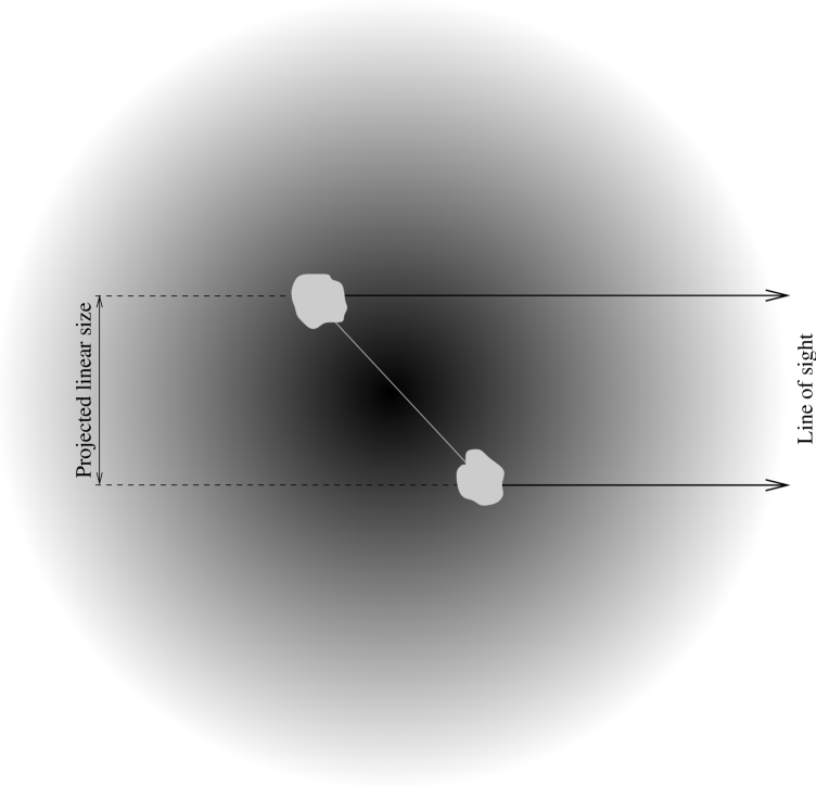
Figure 5: Cartoon of the GPS/CSS geometry used for the modelling of a spherical density distribution. The radio source is confined within the host galaxy, for which we assume a maximum radius of 50kpc, i.e. the ISM diameter is much larger than the largest projected linear size of 10kpc.

4.1 Spherical distribution

The strong radio emission in the GPS/CSS sources is most often concentrated in two lobes, while the core emission (if present) is weak. A cartoon of a GPS/CSS source geometry is shown in Fig. 5. The two lobes do not extend beyond the optical host galaxy, hence the probability of tracing host galaxy ISM should be high, especially if the central environment is enriched due to a merger event. Assuming a spherical, radially declining density distribution of the ISM gas, the larger sources will probe lower density gas. In order to see if such a density distribution could explain the anti-correlation in our data, we calculate the expected integrated absorption $N_{\rm HI}=\int n(r)dl$ towards the two lobes, where $dl$ corresponds to the path of absorption along the line of sight. In this estimate we use a source with an inclination of 45^∘, however, for this symmetric model the resulting Hi column density is only weakly dependent on the inclination.

A first approach is to assume that the density follows a King profile:

$$n=n_{\rm 0}(1+\frac{r^{\rm 2}}{r_{\rm c}^{\rm 2}})^{\rm-\beta}$$ (1)

where $r_{\rm c}$ is the core radius of the gas distribution and $n_{\rm 0}$ is is the density at 1 kpc. From X-ray data, which traces the ionised gas component, the core radius for ellipticals is usually derived to be $\sim$ 1 kpc (Trinchieri et al. trinchieri86 (1986); Forman et al. forman85 (1985)). We consider the simplest case, that the atomic gas component is a constant fraction of the ionised gas and follows a similar profile. The two variable parameters to be constrained are $n_{\rm 0}$ and $\beta$, and we test the goodness of the fit by calculating the sum of squares for the observed and calculated Hi column densities. The best fit to the data is then achieved for $n_{\rm 0}=$ 0.05 cm^-3 and $\beta=$ 1.06. The resulting absorbed Hi column density as a function of source size is plotted with the dotted line in Fig. 7 (calculated for a core radius of 1 kpc and host ISM outer radius of 50 kpc). In this figure the observed values in our sample are plotted with triangles. The King model has a more or less uniform density in its centre, thus for any value of $\beta$ such a density model is unable to reproduce the slope in the data at small linear sizes. The only possibility to reproduce the observed data is to reduce the core radius by several orders of magnitude and, in addition, to increase the core density above 100 cm^-3. However, then the density model does not follow a typical King ISM profile any longer.

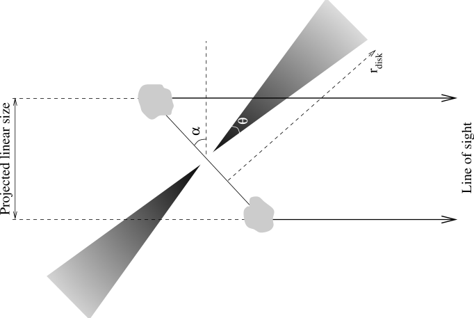
Figure 6: Cartoon of the GPS/CSS geometry used for the disk modelling (not to scale). The disk model is dependent on the disk opening angle $\theta$ and the viewing angle $\alpha$, see Sect. 4.2.

A King model of the density appears inconsistent with not only our data, but also with what is generally assumed for the medium in which the GPS sources expand. More often a simple, steep power law is used, and such power laws successfully explain the detection rates of sources of different sizes (e.g. Fanti et al. fanti95 (1995); Readhead et al. readhead96 (1996); O’Dea & Baum odea97 (1997)). Therefore we instead assume a power law density profile

$$n=n_{\rm 0}(\frac{r}{r_{\rm 0}})^{\rm-\beta}$$ (2)

where $n_{\rm 0}$ is the number density (in cm^-3) at $r_{\rm 0}=$ 1 kpc. We again construct a sum of squares surface, which gives a best fit to the data for $\beta\simeq$ 1.40 and $n_{\rm 0}=$ 0.009 cm^-3(this best fit is plotted in Fig. 7). Assuming a volume filling factor of unity, the integrated Hi mass within a radius of 10 kpc can then be estimated to be 7$\times 10^{7}$ M_⊙. We note that if the filling factor is less than 1, the estimated mass will decrease, and our estimated Hi mass is thus an upper limit. Since the host galaxies of GPS/CSSs may preferentially be found in merging/interacting systems (de Vries et al. devries00 (2000); O’Dea et al. odea96 (1996)), it is interesting to compare the mass of Hi with what has been found in the more nearby population of the luminous infra-red galaxies (ULIRGs). Those sources are also associated with interactions (although between gas rich galaxies), and more or less all of them are detected in Hi emission with masses in the range of 5$\times 10^{8}$ to 3$\times 10^{10}$ M_⊙, with typical values of the order of $10^{9}$ M_⊙ (Mirabel & Sanders mirabel88 (1988)). Even though our objects may also be merging systems, a spherical distribution indicates that the GPS/CSSs are less gas rich than the ULIRGs.

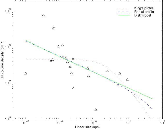
Figure 7: Results of calculating the expected Hi column density given different density profiles. The triangles represents the real data. The King density profile, plotted with a dotted line, cannot reproduce the same Hi column density distribution for any value of $\beta$. Instead, using a power law drop of the density provides a more similar distribution, with the closest fit for $\beta$= 1.40 and $n_{\rm 0}=$ 9$\times 10^{-3}$ cm^-3 (dashed line). Any kind of disk model can fit the data reasonably well, here a disk opening angle of 20^∘ is plotted (solid line).

Given that the host galaxies of radio loud sources are ellipticals, it is also interesting to compare our derived gas mass with what is found in nearby non-AGN ellipticals. Around 15% of those normal ellipticals are detected in Hi emission with masses $M_{\rm HI}\ga$ $10^{9}$ M_⊙ (Huchtmeier et al. huchtmeier95 (1995); Knapp et al. knapp85 (1985)). Typical upper limits of the remaining 85% are of the order of $10^{8}$ – $10^{9}$ M_⊙. Given the sensitivity of the Hi emission experiments, the Hi mass we calculate assuming a spherical power law density profile is consistent with our GPS/CSS sources being hosted by normal ellipticals.

4.2 Disk distribution

Instead of spherically distributed gas, another plausible distribution is a disk in a plane roughly perpendicular to the radio source. For most source orientations this means that only the far radio lobe is occulted. It has been shown from VLA and ATCA Hi imaging that early-type E and S0 galaxies often have their Hi in disk systems (e.g. Sadler et al. sadler00 (2000); Oosterloo et al. oosterloo99 (1999)). Many large scale radio sources show Hi absorption that is consistent with circumnuclear gas, extended on scales of a few pc in radio loud FRIs up to scales of a few 100 pc in low luminosity Seyferts (e.g. van Langevelde et al. vanlangevelde00 (2000); Taylor taylor96 (1996); Gallimore et al. gallimore99 (1999); Vermeulen et al. vermeulen02 (2002)). HST imaging has revealed nuclear disks of gas and dust in radio loud AGN (Verdoes Kleijn et al. verdoes99 (1999); de Koff et al. dekoff00 (2000)). In particular recent HST observations of a few GPS/CSS sources have shown them to contain central disks of gas and dust (4C 31.04, 1946+708 and 1146+596; Perlman et al. perlman01 (2001)). Other high resolution absorption studies of nearby GPSs show that the Hi data are consistent with a rotating ring (e.g. in 1946+708; Peck et al. peck99 (1999) and 4C 31.04; Conway conway96 (1996)). Here we consider the case of the absorbing gas in a disk oriented perpendicular to the radio axis.

In this case absorption will only be seen against the far lobe. For a cartoon image of the simple disk see Fig. 6. The maximum radius of the disk, $r_{\rm disk}$, is assumed to be at least 10 kpc and thus for sources of projected linear sizes up to 10 kpc the far lobe is always covered by the disk. When calculating the Hi column densities, we assume the disk has a radial density profile $n=n_{0}(r/r_{\rm 0})^{-\beta}$, where $n_{\rm 0}$ is the density at $r_{\rm 0}=1$ kpc. The calculated column densities will be a function of both viewing angle as well as the disk opening angle. In our modelling we limit ourselves to a viewing angle of 45^∘, and uses disk opening angles of 10°, 20° and 30°. We again test the goodness of fit using the sum of squares method. Given the scatter in the data all such opening angles give similar fits, and in Fig. 7 we plot the best fit for a disk full opening angle of 20°, yielding $n_{0}=0.11$ and $\beta=1.45$.

A 10kpc radius disk will, assuming there is an inner radius of the disk of 1pc, yield an atomic mass of the order of $10^{8}$ M_⊙. This is comparable to the results of the spherical distribution (Sect. 4.1). Following the discussion in Sect. 4.1, we find that also for a disk distribution the GPS/CSSs appear to be less gas rich than the ULIRGs.

5 Comparison with GPS/CSS models

Currently the most favoured explanation to the small sizes of most GPS and CSS sources is that they are young, as estimated both from their measured expansion speed as well as from synchrotron ageing (e.g. Owsianik & Conway owsianik98a (1998); Murgia et al. murgia99 (1999)). In this ’youth’ scenario the dense gas interacts with the radio plasma giving a large radio luminosity which then explains the relatively larger number of sources with small size. In order to explain the number density of sources of a given size, the radio jet is assumed to propagate in a medium with decreasing density, approximated with a power law profile $\propto r^{\rm-\beta}$ with a slope $\beta=$ 1.5 – 2 (Fanti et al. fanti95 (1995); Begelman begelman96 (1996), Readhead et al. readhead96 (1996)). Given our uncertainties, it is interesting that this exponent is comparable with the $\rm\beta\simeq$ 1.4 we get from our Hi absorption.

Alternatively the GPS/CSSs have been suggested to be old ’frustrated’ sources prevented from growing by a very dense medium (e.g. van Breugel et al. vanbreugel84 (1984); Fanti et al. fanti90 (1990)). In Sect. 1 we mentioned several observations showing the presence of gas in GPS/CSSs. Other evidence for dense environments comes from effects thought to derive from interactions with the surrounding medium, several CSS objects for example display distorted radio morphologies (e.g. van Breugel et al. vanbreugel84 (1984)) and alignment effects between the radio axis and the optical emission (e.g. de Vries et al. 1997b ). Obviously, there is compelling evidence for dense gas in GPS/CSS sources; the question is whether the central density is large enough to give frustration.

While the frustration model is now less popular it is still possible that a minority of the GPS/CSS sources are created in this way. Here we discuss our Hi results in context of those two models.

5.1 The frustration scenario

Table 4: Density of the medium where the lobes expand, as expected from lobe advance speed ($n_{\rm ext}$), compared to Hi density estimates from a spherical density model ($n_{\rm S,100K}$) and a disk model ($n_{\rm D,1000K}$). Estimates are done using $h=0.75$. The first part of the table lists sources which are detected in Hi absorption, while the second part lists sources that are not detected in Hi absorption.

	Source	radius	$v_{\rm a}$	$p_{\rm i}$	ref1	$n_{\rm ext}$	$C_{\rm HI}$	$n_{\rm S,100K}$	$n_{\rm D,1000K}$
		kpc	$h^{\rm-1}\,c$	$h^{\rm 4/7}$dy cm-2	cm-3		cm-3	cm-3
Sources with	J0111+3906	0.017	0.098	1.1$\times 10^{-4}$	1	3.6	9.1	24.6	368.4
detected Hi absorption	J1407+2827	0.005	0.050	2.5$\times 10^{-4}$	2,3	31.8	0.1	1.5	23.9
	J1944+5448	0.087	0.210	2.5$\times 10^{-4}$	4,5	1.8	1.1	0.3	4.2
	J2355+4950	0.078	0.101	9.7$\times 10^{-5}$	6,7	3.0	0.7	0.2	3.1
Sources without	J0713+4349	0.058	0.126	1.9$\times 10^{-4}$	8,7	3.8	…	0.5	6.8
detected Hi absorption	J1035+5628	0.082	0.310	2.9$\times 10^{-5}$	9	0.1	…	0.3	4.1
	J2022+6136	0.011	0.060	6.4$\times 10^{-4}$	10	56.5	…	5.0	76.1

1References for lobe advance speed and the lobe pressure: 1) Owsianik et al. owsianik98b (1998), 2) Polatidis & Conway polatidis03 (2003),
3) Stanghellini et al. stanghellini97 (1997), 4) Polatidis et al. polatidis99 (1999), 5) A. Polatidis, pers. comm., 6) Owsianik et al. owsianik99 (1999),
7) Conway et al. conway92 (1992), 8) Owsianik & Conway owsianik98a (1998), 9) Taylor et al. taylor00 (2000) and 10) Tschager et al. tschager00 (2000)

In order to confine a median luminosity CSS, an average number density in the range 1 – 10 cm^-3 at $r=$ 10 kpc is needed (de Young deyoung93 (1993)). This implies, for a uniform density, gas masses of the order of $10^{10}$ M_⊙. In our power law density model we derive atomic gas masses of the order of $10^{8}$ M_⊙, two orders of magnitude less. Comparison of molecular data with Hi data for elliptical galaxies have indicated a $M_{\rm H2}/M_{\rm HI}$ ratio of the order of 0.4 (Wiklind et al. wiklind95 (1995)). If such a number is applicable also to the GPS/CSS sources, it implies total gas masses around a few times $10^{8}$ M_⊙. This result may change if the ratio $M_{\rm H2}/M_{\rm HI}$ is very different. For the gas rich ULIRGs however, the total molecular gas mass derived from CO emission, and the atomic gas mass derived from Hi emission are of the same order ($10^{9}$ M_⊙; Downes & Solomon downes98 (1998); Mirabel & Sanders mirabel88 (1988)), and will thus change the resulting total gas mass by a small factor. Given those estimates, the Hi absorption data suggests that there is not enough gas to frustrate the radio sources.

5.2 The youth model

The young ages estimated from the hotspot advance speeds are strong arguments in favour of the youth model. Using ram pressure arguments, the lobe advance speed $v_{\rm a}$ is related to the external mass density $\rho_{\rm ext}$ and the hotspot pressure $p_{\rm i}$ by

$$p_{\rm i}=\rho_{\rm ext}v_{\rm a}^{\rm 2}=n_{\rm ext}m_{\rm p}v_{\rm a}^{\rm 2}$$ (3)

Thus, for sources with measured expansion velocities, we can estimate the density $n_{\rm ext}$ at the hotspot location. We can further compare $n_{\rm ext}$ with the density expected using the power law density distribution models discussed in Sect. 4.

Published in the literature we find a selection of 7 sources with measured advance speeds and quoted (or sufficient information to calculate) internal hotspot pressures. For those sources, we list in Table 4 the distance between the core and hotspot, the advance speed, hotspot pressure and the corresponding references. We use Eq. (3) to derive external densities $n_{\rm ext}$ (Table 4) at the given hotspot radius.

In order to derive densities using the disk and spherical power law density profile (Eq. (2)), we first note that all sources listed in Table 4 have very small linear sizes. Especially, for sources $<0.1$ kpc there are large offsets between the measured Hi column density and the Hi column density as predicted by our simple models (Fig. 7). For the sources with measured Hi column density, we therefore apply a correction factor ($C_{\rm HI}=N_{\rm HI,measured}/N_{\rm HI,predicted}$), in order to better estimate the density in the source in question. We also note that the estimated density will depend on the spin temperature; the values for the column density used in Sect. 3 assumes a $T_{\rm sp}=100$K. However, close to an X-ray irradiating AGN the spin temperature is likely to be above 100K, and probably closer to 8000 K if the gas is purely atomic (Maloney et al. maloney96 (1996)).

For the spherical density profile, we use the power law profile (Eq. (2)) and express the density $n_{\rm S}$ as a function of radius and spin temperature:

$$n_{\rm S}=C_{\rm HI}n_{\rm HI}(\frac{T_{\rm sp}}{100\rm K})=C_{\rm HI}n_{\rm 0}r_{\rm kpc}^{-\beta}(\frac{T_{\rm sp}}{100\rm K})$$ (4)

Applying the best fitting values of $n_{0}$ and $\beta$ from Sect. 4.1, and using a spin temperature of 100K we achieve:

$$n_{\rm S,100K}\simeq C_{\rm HI}$\leavevmode\nobreak\ 0.009$r_{\rm kpc}^{\rm-1.4}$$ (5)

At a given radius Eq. (5) gives the Hi density, and is thus a lower limit to the total density. Using the radius of the sources in Table 4, we calculate the corresponding values of the density $n_{\rm S,100K}$. For this model we have chosen to use $T_{\rm sp}=100$K, since that gives the closest match to the densities $n_{\rm ext}$ estimated from the ram-pressure argument. If the spin temperature is 8000 K, the estimated $n_{\rm S}$ will be 80 times higher.

If instead the absorbing gas is in a disk distribution, we can estimate the density at the hotspots (which must be in a medium external to the disk, see Fig. 6) by assuming that the disk internal pressure will be similar to the pressure outside the disk. Since we do not have any information on the properties of such a disk, we will first consider the simplest case, assuming the disk to be completely atomic and to have an uniform kinetic temperature $T_{\rm disk}=T_{\rm sp}$. The external medium is assumed to be ionised with an electron temperature $T_{\rm ext}=$ $10^{4}$ K. Applying the ideal gas law the external density $n_{\rm D}$ can be written as:

$$n_{\rm D}=C_{\rm HI}n_{\rm HI}(\frac{T_{\rm sp}}{100\rm K})(\frac{T_{\rm sp}}{T_{\rm ext}})=C_{\rm HI}n_{\rm 0}r_{\rm kpc}^{\rm-\beta}(\frac{T_{\rm sp}}{100\rm K})(\frac{T_{\rm sp}}{T_{\rm ext}})$$ (6)

For a disk opening angle of 20°, we derived a value of $n_{\rm 0}=$ 0.11 cm^-3 and $\beta=$ 1.45 (Sect. 4.2), and assuming a spin temperature of 1000K we rewrite Eq. (6) into

$$n_{\rm D,1000K}\simeq\leavevmode\nobreak\ 0.11\leavevmode\nobreak\ C_{\rm HI}r_{\rm kpc}^{\rm-1.45}$$ (7)

Again, this is a lower limit to the total gas density present. In order to get densities which best agree with those estimated via the ram pressure argument, we here use a $T_{\rm sp}=1000$K. The resulting values of $n_{\rm D,1000K}$ are listed in Table 4.

Excluding J0111+3906, for the spherical power law model most $n_{\rm ext}$ and $n_{\rm S,100K}$ values are remarkably similar, and in most cases only differ within an order of a magnitude; which is consistent with the GPSs propagating through a purely atomic spherical gas distribution. The offset can depend on a number of things. Firstly, it is possible that the spin temperature has a very different value. Secondly, and closely linked to the spin temperature, is the expected molecular abundance. If the kinetic temperature is as low as 100K, the molecular abundance is expected to be high (Maloney et al. maloney96 (1996)), and thus our Hi density estimate is only a lower limit to the total gas density. Thirdly, the value of $\beta$ and $n_{\rm 0}$ could be different, given the sparse amount of data used in the fitting (22 points). Within a 90% confidence region the value of $\beta$ may change as much as $\pm$0.25 and $n_{\rm 0}$ as much as $\pm$4e-3, with a corresponding difference of $\sim$ 1 in the number density at a radius of 0.05 kpc. Finally the individual viewing angles of the sources in Table 4 may affect the assumed radius where the hotspot is located.

The densities derived from the disk profile are equally similar, differing with only a factor of a few from $n_{\rm ext}$ (except for J0111+3906). The offsets are not surprising, given the large number of uncertainties in the calculation of $n_{\rm D,1000K}$. In addition to the reasons already given for the spherical distribution, the ratio $T_{\rm disk}/T_{\rm ext}$ could for instance be very different from the assumed value.

We conclude that within the scope of the power law profile, we more or less can reproduce the densities expected in the youth model for the GPS sources with measured lobe velocities.

6 Orientation effects on the observed HI
column density: galaxies versus quasars

Figure 8: Hi column density versus fraction of core emission $f_{\rm c}$. Quasars are marked with crosses, and galaxies with squares. In general the quasars are found in sources with larger core prominence, consistent with smaller viewing angles.

In most cases the spatial resolution of present Hi data is not enough to determine whether the absorption covers both lobes (consistent with ISM gas) or only one lobe (indicating a disk distribution). In the previous sections we showed that, given the limited information we have about the density profiles, both a disk as well as a spherical distribution are consistent with the observed relation between Hi column density and linear size. One possibility to distinguish between those models is to look at any possible orientation effects. Assuming the unified scheme, quasars are supposed to be seen at a smaller viewing angle $\alpha$ (more end-on) than the radio galaxies. In fact, we have shown that there appears to be a larger detection rate in galaxies than in quasars (Sect. 3.1).

For a given projected source size of 1 kpc, the amount of expected Hi absorption as a function of viewing angle can be estimated. Given that for a projected size of 1 kpc we have a Hi column density sensitivity of around $10^{20}$ cm^-2 (Fig. 1), the spherical density profile predicts we would detect equal column densities in galaxies (with say $\alpha\ga$ 45°; Barthel barthel89 (1989)) and quasars ($\alpha\la$ 45°). In contrast for the disk profile there will be a range of optimum viewing angles, for which we are likely to detect Hi absorption. This exact range of viewing angles will be extremely dependent on the disk model used. In Sect. 6.1 we discuss if the galaxies and quasars in our sample are consistent with having different viewing angles, as expected from unified schemes. If so, a spherically symmetric distribution could be considered less likely, since objects classified as galaxies appear to have higher Hi column densities than quasars.

6.1 Core prominence

Because of relativistic boosting the core strength is considered to be a good indicator of orientation; the more dominant the core is, the smaller the viewing angle. For larger radio sources, this has been investigated by a number of people (e.g. Orr & Browne orr82 (1982)). Since the GPS/CSS objects in general have weak or no core emission, similar studies have been difficult. Stanghellini et al. (stanghellini01 (2001)) reports on VLBA observations of 10 GPS sources. The authors conclude that in the few cases where cores were detected, the core of the GPS galaxies accounted for $\simeq 2$% of the total flux density, while in the GPS quasars the core accounted for $\simeq 20$%. Moreover, Saikia et al. (saikia95 (1995)) studied a sample of CSS sources with detected radio cores, and found that the degree of core prominence were consistent with those for larger radio sources and also consistent with the unified scheme. In the study by Saikia et al. (saikia95 (1995)), there are 7 sources that can also be found in our sample (3 quasars and 4 galaxies). For the galaxies the average fraction of emission from the core is $\overline{f}_{\rm c}=$ 0.012, while the corresponding number for the quasars is $\overline{f}_{\rm c}=$ 0.26. In Fig. 8 we plot the Hi column density versus $f_{\rm c}$ for those objects, and we mark quasars and galaxies with different symbols. Clearly the quasars have larger core prominence. This implies the quasars have a smaller viewing angle.

Only one of these quasars is detected in Hi absorption, while three of the galaxies are Hi absorbers. For the sources in common with the sources of Saikia et al. (saikia95 (1995)), it appears as if the upper limits of the Hi column density for the quasars are smaller than the detections for the radio galaxies. It would be interesting to carry out deeper observations for a larger sample of the CSS quasars with upper limits; if deeper searches showed (for a majority of the sources) lower column densities or upper limits for the quasars than for the radio galaxy detections, this would strongly argue for a disk origin for the Hi absorption.

6.2 GPS quasars versus GPS galaxies

It should be noted that it is debated whether the GPS quasars are really intrinsically small sources like the GPS galaxies. Snellen (snellen97 (1997)) proposes that GPS galaxies viewed end-on will have a flat spectra and thus the GPS galaxies and quasars are different types of objects. This has some support in a very different redshift distribution for the GPS galaxies and quasars (Snellen snellen97 (1997); Stanghellini stanghellini98 (1998)), and the fact that many GPS quasars appear to have core-jet morphologies when observed at high angular resolution (Stanghellini stanghellini01 (2001)). If this is the case, the low detection rate in the GPS quasars reported here could be explained by them being large scale radio sources, hence with a lower probability of the line of sight going through the host galaxy.

7 Implications for the spectral turn-over mechanism

The integrated radio spectrum turn-over frequency for GPS/CSS sources is known to have a relationship $\nu_{\rm t}\propto LS^{-0.65}$ (O’Dea & Baum odea97 (1997)). Most often this is ascribed to synchrotron selfabsorption (e.g. O’Dea & Baum odea97 (1997)); however an alternative possibility is the one of free-free absorption (e.g. Bicknell et al. bicknell97 (1997)). A few VLBI results indicate the presence of a nuclear disk causing free-free absorption (Marr et al. marr01 (2001); Peck et al. peck99 (1999)).

Since our Hi results show that the column density along the line of sight depends on the source linear size (and thus turnover frequency), it is likely that a similar relationship exists for an ionised gas component. The free-free absorption turn-over frequency is related to the electron density, $\nu_{\rm t}\propto(n_{\rm e}^{2})^{1/2.1}$. If we simply assume the gas fraction to be constant ($n_{\rm HI}/n_{\rm e}=C$) and $N_{\rm HI}=n_{\rm e}L$ where L is the absorbing pathlength, the observed relationship ($N_{\rm HI}\propto LS^{-0.43}$) implies a free-free absorption caused turnover relationship $\nu_{\rm t}\propto LS^{-0.41}$. This is much less steep than observed ($\nu_{\rm t}\propto LS^{-0.65}$), implying that free-free absorption can not be the only turn-over mechanism present.

Conversely we could assume that the observed relationship between turnover frequency and linear size is due to free free absorption. Then, $\nu_{\rm t}\propto LS^{-0.65}$ implies that the slope for the ionised gas component necessarily is larger than the slope we observe for Hi. In this case perhaps there is a gradient of the fraction of ionised gas decreasing with radius.

8 Conclusions

We have investigated the combined results of Hi absorption in GPS/CSS sources. The most striking result is that the smaller GPS sources ($<$ 0.5 kpc) tend to have larger Hi column densities than the larger CSS sources ($>$ 0.5 kpc). This anti-correlation between linear size and absorbed Hi column density is mostly an effect from opacity differences rather than line width differences. It is possible to use a simple power law profile of the density to explain the observed Hi column densities, and both a spherically symmetric medium as well as disk can be fitted to the data.

Our modelling cannot distinguish between the spherical and disk density models, and most observations at present do not have enough resolution to determine the location of the absorbing gas. However, to date high resolution Hi data exist for a limited number of sources that in all cases indicate Hi disks (Conway conway96 (1996); Peck et al. peck99 (1999); Peck & Taylor peck98 (1998)). This argues for a disk model, and in addition we notice that most Hi absorbers are found in sources classified as galaxies. By studying our sources in their radio continuum properties we find that the galaxies and quasars in our sample behave similarly to larger scale sources, where orientation effects are known to take place. Therefore, it is easier to argue for a disk model, where sources with very small viewing angles in addition to sources observed edge-on would be less likely to have Hi detectable in absorption against their lobes. The fact that quasars have smaller column densities argues against a spherically symmetric model for the Hi gas.

- (1) Bahcall, J. N., Kirhakos, S., Saxe, D. H., & Schneider D.P. 1997, ApJ, 479, 642
- (2) Barthel, P. D. 1989, ApJ, 336, 606
- (3) Begelman, M. C. 1996, in Cygnus A - a Study of a Radio Galaxy, ed. C. L. Carilli, & D. E. Harris, Cambridge University Press, 209
- (4) Bicknell, G. V., Dopita M. A., & O’Dea, C. P. 1997, ApJ, 485, 112
- (5) Carilli, C. L., Perlman, E. S., & Stocke J. T. 1992, ApJ, 400, L13
- (6) Carilli, C. L., Menten, K. M., Reid, M. J., Rupen, M. P., & Yun, M. S., 1998, ApJ, 494, 175
- (7) Conway, J. E., Pearson, T. J., Readhead, A. C. S., et al. 1992, ApJ, 396, 62
- (8) Conway, J. E. 1996, in The Second Workshop on Gigahertz Peaked Spectrum and Compact Steep Spectrum Radio Sources, ed. I. Snellen, R.T. Schilizzi, H. A. J. Röttgering, & M. N. Bremer, Publ JIVE, Leiden, 198
- (9) de Koff, S., Best, P., Baum, S. A., et al. 2000, ApJS, 129, 33
- (10) de Vries, W. H., Barthel, P. D., & O’Dea, C. P. 1997, A&A, 321, 105
- (11) de Vries, W. H., O’Dea C.P., Baum, S. A., et al. 1997, ApJS, 110, 191
- (12) de Vries, W. H., O’Dea, C. P., Barthel P.D., et al. 2000, ApJ, 120, 2300
- (13) de Young, D. S., 1993, ApJ, 405, L13
- (14) Downes, D., & Solomon, P. M. 1998, ApJ, 507, 615
- (15) Dunlop, J. S., McLure, R. J., Kukula, M. J., Baum, S. A., O’Dea, C. P., & Hughes, D. H. 2003, MNRAS in press, see astro-ph/0108397
- (16) Elvis, M., Fiore, F., Wilkes, B., McDowell, J., & Bechtold, J. 1994, ApJ, 422, 60
- (17) Evans, A. S., Kim, D. C., Mazzarella, J. M., Scoville, N. Z., & Sanders, D. B. 1999, ApJL, 521, L107
- (18) Fanti, R., Fanti C., Schilizzi, R. T., et al. 1990, A&A, 231, 333
- (19) Fanti, C., Fanti, R., Dallacasa, D., et al. 1995, A&A, 302, 317
- (20) Forman, W., Jones, C., & Tucker, W. 1985, ApJ, 293, 102
- (21) Gallimore, J. F., Baum, S. A., O’Dea, C. P., Pedlar, A., & Brinks, E. 1999, ApJ, 524, 684
- (22) Gelderman, R., & Whittle, M. 1994, ApJS, 91, 491
- (23) Huchtmeier, W. K. 1994, A&A, 286, 389
- (24) Huchtmeier, W. K., Sage, L. J., & Henkel, C., 1995, A&A, 300, 675
- (25) Isobe, T., Feigelson, E. D., & Nelson, P. I., 1986, ApJ, 306, 490
- (26) Kameno, S., Horiuchi S., Shen, Z.-Q., et al. 2000, PASJ, 52, 209
- (27) Kato, T., Tabara, H., Inoue, M., & Aizu, K. 1987, Nature, 329, 223
- (28) Knapp, G. R., Stark, A. A., & Wilson, R. W. 1985, AJ, 90, 254
- (29) Lavalley, M., Isobe, T., & Feigelson, E. 1992, BAAS, 24, 839
- (30) Leon, S., Lim, J., Combes, F., & Van-Trung, D. 2001, in QSO Hosts and Their Environments’, ed. I. Marquez, preprint
- (31) Lim, J., Leon, S., Combes, F., & Dinh-V-Trung, D. 2000, ApJ, 545, L93
- (32) Maloney, P. R., Hollenbach D. J., & Tielens A. G. G. M. 1996, ApJ, 466, 561
- (33) Marr, J. M., Taylor, G. B., & Crawford, F. III 2001, ApJ, 550, 160
- (34) Martel, A. R., Baum, S. A., Sparks, W. B., et al. 1999, ApJS, 122, 81
- (35) Mirabel, I. F., & Sanders, D. B. 1988, ApJ, 335, 104
- (36) Mirabel, I. F., 1989a, ApJ, 340, L13
- (37) Mirabel, I. F., Sanders, D. B., & Kazes, I. 1989b, ApJ, 340, L9
- (38) Morganti, R., Oosterloo, T. A., Reynolds, J. E., Tadhunter, C.N., & Migenes, V. 1997, MNRAS, 284, 541
- (39) Murgia, M., Fanti, C., Fanti, R., et al. 1999, A&A, 345, 769
- (40) O’Dea, C. P., Stanghellini, C., Baum, S., & Charlot, S. 1996, ApJ, 470, 806
- (41) O’Dea, C. P., & Baum, S. A. 1997, AJ, 113, 148
- (42) Oosterloo, T. A., Morganti, R., & Sadler, E. 1999, PASA, 16, 28
- (43) Orr, M. J. L., & Browne, I. W. A. 1982, MNRAS, 200, 1067
- (44) Owsianik, I., & Conway, J. E. 1998, A&A, 337, 69
- (45) Owsianik, I., Conway, J. E., & Polatidis, A. G. 1998, A&A, 336, L37
- (46) Owsianik, I., Conway, J. E., & Polatidis, A. G. 1999, New Astronomy Reviews, 43, 669
- (47) Parma, P., Murgia, M., Morganti, R., et al. 1999, A&A, 344, 7
- (48) Peck, A. B., & Taylor, G. B. 1998, ApJ, 502, L23
- (49) Peck, A. B., Taylor, G. B., & Conway, J. E. 1999, ApJ, 521, 103
- (50) Peck, A. B., Taylor, G. B., Fassnacht, C. D., Readhead, A. C. S., & Vermeulen, R. C. 2000, ApJ, 534, 104
- (51) Perlman, E. S., Stocke, J. T., Conway, J. E., & Reynolds, C. 2001, AJ, 122, 536
- (52) Polatidis, A. G., & Conway, J. E. 2003, PASA, vol 20
- (53) Polatidis, A., Wilkinson, P. N., Xu, W., et al. 1999, New Astronomy Reviews, 43, 657
- (54) Readhead, A. C. S., Taylor, G. B., Pearson, T. J., Wilkinson, P. N. 1996, ApJ, 460, 634
- (55) Sadler, E. M., Oosterloo, T. A., Morganti, R., & Karakas, A. 2000, AJ, 119, 1180
- (56) Saikia, D. J., Jeyakumar, S., Wiita, P. J., Sanghera, H. S., & Spencer, R. E. 1995, MNRAS, 276, 1215
- (57) Spencer, R. E., McDowell, J. C., Charlesworth, M., et al. 1989, MNRAS, 240, 657
- (58) Snellen, I. A. G., PhD Thesis, Univ. of Leiden
- (59) Snellen, I. A. G., Schilizzi, R. T., Miley, G. K., de Bruyn, A. G., Bremer, M. N., & Röttgering, H. J. A. 2000, MNRAS, 319, 445
- (60) Stanghellini C., Bondi M., Dallacasa D., et al. 1997, A&A, 318, 376
- (61) Stanghellini, C., O’Dea, C. P., Dallacasa, D., et al. 1998, A&AS, 131, 303
- (62) Stanghellini, C., Dallacasa, D., O’Dea, C. P., et al. 2001, A&A, 377, 377
- (63) Taylor, G. B., Marr, J. M., Pearson, T. J. & Readhead, A. C. S. 2000, ApJ, 541, 112
- (64) Taylor, G. B. 1996, ApJ, 470, 394
- (65) Tschager, W., Schilizzi, R. T., Röttgering, H. J. A., Snellen, I. A. G., & Miley, G. K. 2000, A&A, 360, 887
- (66) Trinchieri, G., Fabbiano, G., & Canizares, C. R. 1986, ApJ, 310, 637
- (67) van Breugel, W., Miley, G., & Heckman, T., 1984, AJ, 89, 5
- (68) van Gorkom, J. H., Knapp, G. R., Ekers, R. D., et al. 1989, AJ, 97, 708
- (69) van Langevelde, H. J., Pihlström, Y. M., Conway, J. E., Jaffe, W., & Schilizzi, R. T. 2000, A&A, 354, L45
- (70) Verdoes Kleijn, G. A., Baum, S. A., de Zeeuw, P. T., & O’Dea, C. P. 1999, AJ, 118, 2592
- (71) Vermeulen, R. C., Ros, E., Kellermann, K. I., et al. J. A. 2002, PASA 20, in press
- (72) Vermeulen, R. C., Pihlström Y.M., Tschager W., et al. 2003, A&A, accepted
- (73) Wiklind, T., Combes, F., & Henkel, C. 1995, A&A, 297, 643