Slow evolution of elliptical galaxies induced by dynamical friction
I. Capture of a system of satellites

The main goal of this paper is to set up a numerical laboratory for the study of the slow evolution of the density and of the pressure tensor profiles of an otherwise collisionless stellar system, as a result of the interactions with a minority component of heavier “particles”. The effects that we would like to study are those attributed to slow collisional relaxation and generically called “dynamical friction”; in real cases, or in numerical simulations, the processes involved are complex, so that the relaxation associated with the granularity in phase space is generally mixed with and masked by evolution resulting from lack of equilibrium or from a variety of instabilities and collective processes. We start by revisiting the problem of the sinking of a satellite inside an initially isotropic, non-rotating, spherical galaxy, which we follow by means of N-body simulations using about one million particles. We then consider a quasi-spherical problem, in which the satellite is fragmented into a set of many smaller masses with a spherically symmetric initial density distribution. In a wide set of experiments, designed in order to bring out effects genuinely associated with dynamical friction, we are able to demonstrate the slow evolution of the density profile and the development of a tangentially biased pressure in the underlying stellar system, while we briefly address the issue of the circularization of orbits induced by dynamical friction on the population of fragments. The results of the simulations presented here and others planned for future investigations allow us to study the basic mechanisms of slow relaxation in stellar systems and thus may be of general interest for a variety of problems, especially in the cosmological context. Here our experiments are conceived with the specific goal to clarify some mechanisms that may play a role in the evolution of an elliptical galaxy as a result of the interaction between the stars and a significant population of globular clusters or of the merging of a large number of small satellites.

1 Introduction

If we consider a globular cluster of mass $m_{gc}\sim 10^{5}M_{\odot}$ orbiting inside a spherical galaxy, given the mass ratio $10^{5}$ with respect to the mass of a typical star, we find that it should suffer dynamical friction on a time-scale $T_{fr}\sim 10^{9}$yr, through scattering of the stars. [The term dynamical friction refers to the slow relaxation process associated with discrete two-body encounters investigated in the pioneering studies of Chandrasekhar (cha43 (1943)). In these classical analyses, estimate is given of the cumulative effect of discrete encounters on a test particle passing through a homogeneous system of field particles. This effect, associated with the granularity of the system in phase space, is ignored in pure Vlasov descriptions of stellar systems. The term dynamical friction is often extended to describe loosely the physical origin of orbital decays of satellites of finite mass also in real inhomogeneous systems and simulations, which fall obviously outside the classical description of Chandrasekhar.] If the cluster starts from a circular orbit located at $r_{i}$, in a time $\sim T_{fr}$ it will reach a lower orbit close to $r_{f}$, while a fraction of the energy initially associated with such a cluster $E_{i}=m_{gc}\Phi(r_{i})+(1/2)m_{gc}r_{i}(d\Phi/dr)_{r_{i}}$ is released into the distribution function of the hosting galaxy. If we refer to the realistic possibility of the presence of several thousands of such globular clusters we may thus argue that on a fraction of the Hubble time the underlying stellar system may well absorb a non-negligible fraction of its binding energy and thus should slowly evolve (see also Lotz et al. lot01 (2001)).

Under the suggestive scenario just outlined, the issue we would like to address in this paper is the following conceptually challenging problem. In a two-component system, where the more massive component (the “galaxy”) is basically collisionless and the minority component (the globular cluster system or a large number of mini-satellites caught in minor mergers) is slowly dragged in toward the galaxy center by processes of dynamical friction with the stars of the galaxy, how does the distribution function of the galaxy evolve during the process? A resolution of this challenging problem requires a clarification of the basic mechanism of dynamical friction under inhomogeneous conditions and a discussion of the collective effects involved in the reaction of the underlying distribution function. Note that while the infall of a single cluster (or satellite) is a problem with a preferred direction (given by the angular momentum of the satellite), the capture of a large number of randomly distributed clusters (or mini-satellites) can preserve spherical symmetry, if present to begin with.

It might be argued that the slow evolution in the quasi-isotropic many-cluster case described above could be modeled in terms of an adiabatic evolution of a distribution function within spherical symmetry. For the different problem of the adiabatic growth of a central massive black hole, such a procedure has indeed been developed (e.g., see Cipollina & Bertin cip94 (1994) and references therein). Here it is not clear how a semi-analytic procedure to calculate such slow evolution, taking advantage of the conservation of the relevant actions, can be formulated. In addition, given the relation between dynamical friction and resonant interactions (e.g., see Weinberg wei89 (1989)), in spite of its slowness the process is likely to be inherently non-adiabatic. Therefore, it seems that the only viable way to an answer is that of approaching the problem by means of suitable N-body simulations.

In the long run, results from this project could also shed light on another theoretically interesting scenario, which so far has found major applications only in the context of the internal dynamics of globular clusters. This is a picture, pioneered by Bonnor (bon56 (1956)) in his analysis of gas spheres, by which stellar systems may be subject to a process of gravitational catastrophe (Lynden-Bell & Wood lyn68 (1968)), when their central concentration exceeds a certain threshold value. The catastrophe consists in an instability process, where evolution leads to cores that become more and more concentrated. The source of this instability is thermodynamical, in the sense that it results from a counter-intuitive property of self-gravitating systems, which can be described in terms of negative specific heat. Recently, this general scenario has been demonstrated to hold for an astrophysically interesting family of partially relaxed stellar systems (Bertin & Trenti 2003).

The study of relaxation in N-body simulations and by means of N-body simulations is a vast field of research (e.g., see Hohl hoh73 (1973) and Huang et al. hua93 (1993)). The study of the sinking of a single satellite inside a galaxy, as a result of dynamical friction, was undertaken systematically about two decades ago, initially through simplified simulations, within a restricted three-body problem and with the center of mass of the primary galaxy being kept fixed, and then by means of more realistic, self-consistent simulations (Bontekoe & van Albada bon87 (1987); Zaritsky & White zar88 (1988); Bontekoe bon88 (1988)). The results showed that the general scaling predicted by the classical formulae derived in the “homogeneous limit” (or “local limit”) (Chandrasekhar cha43 (1943)) was basically applicable, although the sinking time scale turned out to be significantly longer (by a factor of $2-3$ for the regimes studied by the numerical experiments) if the self-consistent response of the galaxy was properly incorporated. A convincing interpretation of the sinking process can be made, at least in the limit where the mass of the sinking satellite is small, by investigating the linear response in the galaxy distribution function through stellar dynamical techniques (Fridman & Polyachenko fri84 (1984); Palmer & Papaloizou pal85 (1985); Weinberg wei86 (1986), wei89 (1989); Bertin et al. ber94 (1994), hereafter BPRV94; Palmer pal94 (1994)). Such response consists of an “in-phase” contribution, which has little relevance to the mechanism responsible for dynamical friction, and an “out-of-phase” contribution, associated with the “resonant” interaction, which produces a wake able to set a significant torque on the satellite. These techniques demonstrate that the collective wake in the galaxy, largely dominated by the dipolar ($l=1$) response, can trail significantly away from the orbiting object (when the satellite is outside the galaxy, the response is concentrated around a location opposite to the object with respect to the global center of mass), so that the resulting torque on the satellite that is responsible for dynamical friction can be significantly reduced with respect to other more naive calculations. Discrepancies between earlier simulations and the predictions of the stellar dynamic semi-analytic theory were ascribed to non-linearity effects (in the sense that the satellite-to-galaxy mass ratio $M_{s}/M_{G}\approx 0.1$ considered in the simulations was judged to be excessive; see Hernquist & Weinberg her89 (1989)), but the general picture appears to have been clarified. It is noted that the differences in behavior with respect to the naive expectations of the traditional formulae for dynamical friction become substantial when the size of the satellite is finite (Weinberg (wei89 (1989)) refers to the length ratio $R_{s}/R_{G}$; the multipoles associated with the perturbation with $l$ above a certain threshold are bound to be unimportant), while the differences should become negligible for very compact satellites (in which case all multipoles contribute, with a divergence that is removed by the Coulomb logarithm).

Several aspects of the general problem of dynamical friction have been revisited recently. The issue of the contrast between “local” and “non-local” effects has been re-discussed (Prugniel & Combes pru92 (1992); Maoz mao93 (1993); Cora, Muzzio & Vergne cor97 (1997)), with the confirmation that the description of the friction process in terms of the “homogeneous limit” (Chandrasekhar cha43 (1943)) should be adequate in the limit of low-mass, relatively compact satellites. A very recent investigation (Cora, Vergne & Muzzio cor01 (2001)) also suggests that the process depends very little on the regularity or the stochasticity of the stellar orbits in the galaxy, in contrast with some earlier conjectures (Pfenniger pfe86 (1986)). Other interesting problems are the problem of circularization (of the satellite orbit), the relation of the friction effect to the past history of the dynamical event under consideration, and the issue of a direct calculation of the relevant dissipative force from the response of the stellar system to the perturbing satellite (e.g., see Séguin & Dupraz seg94 (1994, 1996); see also Colpi col98 (1998); Colpi & Pallavicini col98a (1998); Colpi, Mayer & Governato col99 (1999); Nelson & Tremaine nel99 (1999)).

Note that so far investigations of processes of dynamical friction have mostly focused on the issue of the fate of the sinking objects (and mostly for the case of one object; but see Tremaine, Ostriker & Spitzer tre75 (1975)), while the problem of the reaction of the distribution function of the underlying stellar system (especially in the quasi-spherical limit of a system of many heavy objects outlined above) remains practically unexplored.

Our paper is organized as follows. In Sect. 2 we summarize the theoretical framework that allows us to understand the mechanisms of dynamical friction within the context of a single sinking satellite. In Sect. 3 we describe the model adopted. For the present exploratory investigation, the choice of the model (both for the galaxy and for the satellite or the fragments) is mostly dictated by convenience (for the study of dynamical mechanisms and for an easier comparison with previous analyses) rather than by realistic requirements. In Sect. 4 we describe the diagnostic tools that will be used in the simulations and some preliminary tests. In Sect. 5 we proceed to illustrate the results of the simulations for the case of one sinking satellite and for the quasi-spherical case for which the sinking of many smaller mini-satellites is considered. In Sect. 6 we briefly draw our conclusions and set out the plans for future investigations.

2 Theoretical framework for the problem of a single sinking satellite

Here we briefly recall the main issues involved in the problem of a single sinking satellite of “diameter” $2R_{s}$, initially located on a circular orbit at distance $r_{s}\approx R_{G}$ from the center of mass of the entire system. Here $R_{G}$ denotes the “radius” of the galaxy. Let $\Omega_{s}>0$ be the angular velocity of the satellite along its circular orbit. The case of a very compact satellite is likely to be within the reach of the classical formulae for dynamical friction (Chandrasekhar cha43 (1943)). In the case where the satellite is sufficiently extended, for the description of its density distribution and the associated gravitational potential, only the first harmonics in a multipole expansion are important, up to $l_{max}\sim\pi r_{s}/(2R_{s})$ (see Weinberg wei89 (1989)).

A “friction” torque acting on the satellite is expected to result from the action of suitable resonances with star orbits. To understand this, we may refer to the action of the satellite as a perturbation over a basic state that is non-rotating, spherically symmetric, and characterized by isotropic distribution function $f_{0}(E)$, where $E=v^{2}/2+\Phi_{0}(r)$ is the star energy, per unit mass, in the absence of the perturbation, and we may then follow the analysis developed earlier (BPRV94).

Analytical results can be derived in the limit when the mass of the satellite is vanishingly small (with respect to the mass of the galaxy, so that the resulting perturbation in the galaxy distribution function can be treated by a linear theory; see subsection 2.2). In practice, for real systems or for numerical simulations, some of the evolution effects are going to be associated with the finite mass of the satellite. Once we move to consider the possibility of a quasi-equilibrium configuration for a composite system (galaxy plus satellite or a population of mini-satellites), we then have to worry about genuine instabilities that may occur, independent of the granularity present in the system. All of this will contribute to evolution although, in principle, it is not related to the original gedanken experiment at the basis of the classical definition of dynamical friction.

Another subtle aspect of the problem is related to geometry. Broadly speaking, we may think that the difference between the case of straight orbits (considered in the classical description of dynamical friction) and that of orbits in the inhomogeneous potential of the galaxy is taken into account in the following discussion of the resonant response. Yet, the cumulative effects on a single star, because of multiple encounters with the satellite (for example, for stars on quasi-circular orbits), grow in time differently from the classical picture, even before dealing with the collective behavior of the entire set of stars that characterizes the resonant response.

2.1 Single-star Resonances

The frequency $\omega$ associated with the $m$-th component of a multipolar term of order $l$ in the expansion of the potential $\Phi_{s}$ of the satellite is readily related to the angular frequency of the satellite $\omega=-m\Omega_{s}$. Therefore, if we refer to Eq. (80) of BPRV94, we find that the appropriate resonance condition is $-m\Omega_{s}-p\Omega_{r}(E,J)+s\Omega_{\theta}(E,J)=0$; here $s$, $m$, $p$ are integers ($-l\leq s,m\leq+l$; $-\infty<p<\infty$) and $\Omega_{r}(E,J)>0$, $\Omega_{\theta}(E,J)>0$ are the two frequencies (dependent on the star specific energy $E$ and angular momentum $J$) that characterize the star orbit and depend on the properties of the basic state. As discussed in BPRV94, only the components with $s=l,l-2,..-l$ contribute to the density perturbation.

For an extended satellite, the $p=0$ component, which corresponds to an average along the star radial orbit excursion, is expected to dominate so that the resonance condition should reduce to $\Omega_{\theta}(E,J)=m\Omega_{s}/s$. Note that in the course of time, because of dynamical friction, the angular frequency of the satellite is going to change. Clearly, the resonance conditions that we have just stated are applicable provided that $\dot{\Omega}_{s}/\Omega_{s}\ll\Omega_{\theta}(E,J)$, which we can rewrite as $\dot{\Omega}_{s}\ll\Omega_{s}^{2}/l$.

2.2 “Shielding” and global resonances

If we consider the linearized Vlasov-Poisson equation for our problem, we see that Eq. (54) of BPRV94 is modified into $f_{1}=\mathcal{L}(\Phi_{s}+\Phi_{1})$, where $\mathcal{L}$ is a linear operator that basically describes one integration along the unperturbed characteristics. The quantity $f_{1}$ can be called the linear response of the distribution function. This response has a “driven” part, associated with $\Phi_{s}$, and a “self-gravitating” part, related to the potential $\Phi_{1}$, that must be consistent with the response itself, following the Poisson equation $\nabla^{2}\Phi_{1}=4\pi G\int f_{1}d^{3}v$.

In plasma physics, the latter contribution is often called the “shielding” associated with the collective behavior of the plasma. Such shielding is often ignored, although it should be emphasized that this step is improper, because the omitted term is a linear contribution. A relatively simple analysis can then be made, by neglecting the self-gravity of the response, showing the connection between single-star resonances and dynamical friction. Note that this is the only ground where a comparison with Chandrasekhar’s (cha43 (1943)) work can be made.

The general case, which includes the possibility of resonance with discrete global modes of the system, is currently beyond the reach of analytical investigations (see also Vesperini & Weinberg 2000).

3 Model

As a model of the primary stellar system (the “galaxy”), following Bontekoe & van Albada (bon87 (1987)) we consider an isotropic polytropic model of index $n=3$. The distribution function is thus of the form $f_{G}(\@vec{r},\@vec{v})=A(E_{0}-E)^{n-3/2}$ for $E<E_{0}$, with $f_{G}(\@vec{r},\@vec{v})=0$ for $E>E_{0}$, where $E=\Phi_{G}(r)+v^{2}/2$ is the single-star energy, $E_{0}=\Phi_{G}(R)=-GM/R$ is the gravitational potential at the boundary $r=R,$ and $M$ is the total mass of the system. Polytropes can be described in terms of the Lane-Emden function $\theta(\xi),$ which satisfies the differential equation:

$$\frac{1}{\xi^{2}}\frac{d}{d\xi}(\xi^{2}\frac{d\theta}{d\xi})=-\theta^{n},$$ (1)

where $n$ is the polytropic index, with the boundary conditions $\theta=1$, $d\theta/d\xi=0$ at $\xi=0$. From the function $\theta(\xi)$ one can find the potential $\Phi_{G}(r)$ and the associated density $\rho_{G}(r)$.

The secondary object (the “satellite”) is described by a rigid Plummer density distribution (corresponding to a polytrope of index $n=5$), characterized by $\theta=(1+0.5\xi^{2})^{-1/2}$. The potential and the mass distribution of the satellite are then defined by two scales, $R_{s}$ and mass $M_{s}$, so that $\Phi_{s}(r)=-GM_{s}(R_{s}^{2}+r^{2})^{-1/2}$, with cumulative mass $M_{s}(r)=M_{s}r^{3}(R_{s}^{2}+r^{2})^{-3/2}$. This distribution extends to infinity, but 90% of the mass is contained within $3.7R_{s}.$

As a result of the interaction with the satellite, the distribution function of the galaxy is a time-evolving $f$ that will be associated with a mean field $-\nabla\Phi$, to be derived from the Poisson equation $\Delta\Phi(\@vec{r},t)=4\pi G\int fd^{3}v=4\pi G\rho(\@vec{r},t)$. We solve the Poisson equation on a spherical polar mesh of $24\times 12\times 24$ cells in the $r,\theta$, and $\varphi$ directions. The radial mesh is logarithmic. The angular mesh is fixed, with 12 equal divisions in $\cos\theta$ and 24 in $\varphi.$ On this mesh the density, the potential, and the force field are expanded in associated Legendre functions $P_{l}^{m}(\cos\theta)$ up to $P_{6}^{6}.$ At each time-step the center of the spherical mesh used to calculate the potential and the force field in the galaxy is repositioned so as to coincide with the center of mass of the galaxy. The equations of the motion (for the particles representative of the galaxy and, separately, for the satellite) are integrated in Cartesian coordinates with the so called leapfrog scheme. This is basically the N-body code described by van Albada & van Gorkom (van77 (1977)) and then improved and used by van Albada (van82 (1982)) and by Bontekoe & van Albada (bon87 (1987)). Therefore, we do not provide here a full description of the method employed, since it is available in the papers quoted.

3.1 Sinking of a single satellite

A first set of numerical experiments addresses the sinking of a single satellite, initially located on a circular orbit at $\theta=\pi/2$.

The galaxy is considered as a collisionless stellar system, so that its representative particles $(i=1,.....,N)$ interact with each other through the mean gravitational potential $\Phi$ and directly with the satellite:

$$\frac{d^{2}\@vec{r}_{i}}{dt^{2}}=-\nabla\Phi(\@vec{r}_{i},t)-\frac{GM_{s}(\@vec{r}_{i}-\@vec{r}_{s})}{[R_{s}^{2}+(\@vec{r}_{i}-\@vec{r}_{s})^{2}]^{3/2}}.$$ (2)

Note that $\Phi$ is updated separately by the Poisson-solver scheme, following the original method described by van Albada & van Gorkom (van77 (1977)) (this step effectively closes the system of equations), which guarantees a pure time-reversible evolution.

In turn, the satellite is taken to interact with all the representative particles of the galaxy directly via two-body forces:

$$\frac{d^{2}\@vec{r}_{s}}{dt^{2}}=\sum_{i=1}^{i=N}\frac{Gm(\@vec{r}_{i}-\@vec{r}_{s})}{\left[R_{s}^{2}+(\@vec{r}_{i}-\@vec{r}_{s})^{2}\right]^{3/2}},$$ (3)

In the equations above, $\@vec{r}_{i},m$ are the position vectors and the mass of the representative particles of the galaxy, while $\@vec{r}_{s}$ is the position vector of the satellite. All position vectors are measured with respect to an inertial frame of reference with its origin at the center of mass of the combined (galaxy + satellite) system.

3.2 Sinking of many fragments

Another set of experiments studies an initial configuration where the satellite is fragmented into several ($N_{f}$) pieces (“mini-satellites” or “fragments”). For simplicity, we take the fragments to be characterized by the same Plummer density distribution with mass $M_{f}$ (such that $M_{s}=N_{f}M_{f}$) and the same lengthscale $R_{f}=R_{s}$ (a smaller lengthscale $R_{f}$ would be more realistic for the astronomical system we have in mind, but would be less easy to simulate).

The mutual interactions between mini-satellites can be kept “on” by considering

$$\frac{d^{2}\@vec{r}_{i}}{dt^{2}}=-\nabla\Phi(\@vec{r}_{i},t)-\sum_{j=1}^{j=N_{f}}\frac{G{M_{f}}(\@vec{r}_{i}-\@vec{r}_{fj})}{[R_{f}^{2}+(\@vec{r}_{i}-\@vec{r}_{fj})^{2}]^{3/2}},$$ (4)

for the representative particles of the galaxy (labeled by $i=1,....,N$), and

$$\frac{d^{2}\@vec{r}_{fj}}{dt^{2}}=\@vec{a}_{j}^{(1)}+\@vec{a}_{j}^{(2)}$$ (5)

for the mini-satellites (labeled by $j=1,...,N_{f}$), where

$$\@vec{a}_{j}^{(1)}=\sum_{i=1}^{i=N}\frac{Gm(\@vec{r}_{i}-\@vec{r}_{fj})}{\left[R_{f}^{2}+(\@vec{r}_{i}-\@vec{r}_{fj})^{2}\right]^{3/2}}$$ (6)

is the acceleration produced by the galaxy and $\@vec{a}_{j}^{(2)}$ denotes the gravitational acceleration exerted on the $j$-th mini-satellite by the other fragments. The gravitational interaction between two extended bodies is complicated to describe. For the purposes of the present paper, where we are not interested in the phenomena associated with the details of such interaction, we simplify the simulations by referring to the following prescription:

$$\@vec{a}_{j}^{(2)}=\sum_{k=1,k\neq j}^{k=N_{f}}\frac{GM_{f}(\@vec{r}_{fk}-\@vec{r}_{fj})}{\left[R_{f}^{2}+(\@vec{r}_{fk}-\@vec{r}_{fj})^{2}\right]^{3/2}}.$$ (7)

All position vectors are measured with respect to an inertial frame with its origin at the center of mass of the entire system.

The mutual interaction between mini-satellites can be ignored and turned “off” simply by taking $\@vec{a}_{j}^{(2)}=0$. This procedure may be the more realistic procedure if we wish to simulate a system of globular clusters inside a galaxy. In fact, for such system, the few-body-problem effects associated with such interaction are expected to play a secondary role.

As to the initial distribution of the fragments we have considered three cases, to be described below. The first is the most natural generalization of the study of the sinking of a single satellite. A posteriori, we have found that in such a case the effects related to the lack of equilibrium in the initial conditions are too strong and confuse the picture of evolution. (Similar problems, related to the lack of equilibrium, were present also in the case of a single satellite, but those are not emphasized in this paper because that case has been well studied in the past and we prefer to focus here on the new quasi-spherical problem in the presence of many fragments). Therefore we have devised quieter starts so as to better disentangle the effects associated with the granularity of the system from those associated with the lack of equilibrium.

Given the relatively small number of fragments involved, we anticipate that different realizations of the physical cases described below may be associated with different evolutions.

3.2.1 I: Fragments quasi-isotropically distributed on circular orbits on a thin shell

We first consider the case where all the fragments are distributed initially with random positions on a thin shell, located at radius $r_{shell}(0)$. The fragments are given initial velocities appropriate for circular orbits, with random orientations, based on the gravitational field generated by the galaxy alone.

The purpose of simulations of this type is to derive information relevant for a more realistic situation where the fragments have a full three-dimensional space distribution, so that the interaction between the galaxy and the minority population is differential with radius. Such ideally desired simulations are not feasible with current codes. To move one step further in the desired direction we have then considered the case of two shells of fragments initially located at different radii.

Unfortunately, due to the finite mass of the set of fragments, these simulations are characterized by violent epicyclic oscillations that shake the system on the fast dynamical time scale and tend to persist long after the initially expected transient.

3.2.2 II: Fragments quasi-isotropically distributed on circular orbits on a thick shell with improved initial conditions

In order to set up a smoother quasi-equilibrium initial condition, we have decided to proceed as follows. We refer to a spherically symmetric density distribution for a shell of the form $\rho_{shell}=\rho_{0}\exp[-(r-r_{shell}(0))^{2}/a^{2}]$ for $|r-r_{shell}(0)|\leq 2a$ (and vanishing for $|r-r_{shell}(0)|>2a$). The normalization constant $\rho_{0}$ is taken in such a way that the total mass associated with the shell is $M_{s}$. In view of the choice of model for the fragments, we have decided to take $2a=R_{s}$.

Such density distribution generates a potential $\Phi_{shell}(r)$, which can be calculated numerically. We now consider a modified distribution function for the galaxy $f_{G}(\@vec{r},\@vec{v})$ taken to be of the polytropic form as in Sect. 3, but with $E=\Phi_{G}(r)+\Phi_{shell}(r)+v^{2}/2$. We then have to integrate a Lane-Emden equation similar to Eq. (1) but modified by the presence of the external potential $\Phi_{shell}(r)$. This yields a potential $\Phi_{G}(r)$ different from that considered in Sect. 3, to be inserted into the definition of $f_{G}(\@vec{r},\@vec{v})$.

Finally, we consider the clumpy realization of the shell density distribution by reducing it to a set of $N_{f}$ fragments of mass $M_{f}$. The $j-$th fragment is initially distributed in $r$ at a location $r_{fj}$ (with random angular coordinates) so that the set of fragments reproduces the assumed density distribution of the shell; its initial velocity is that appropriate for the circular velocity of a test particle in the combined potential $\Phi_{G}(r)+\Phi_{shell}(r)$.

This procedure ensures a quieter start while leaving the basic picture of the single shell case unchanged. It can be generalized to the case of two shells of fragments initially located at different radii.

3.2.3 III: Fragments constructed by clumping part of the galaxy distribution function

The cases considered above are aimed at describing the interaction between the galaxy and a minority component with phase-space properties distinct from those of the galaxy. As we have seen while addressing the need for a quieter start, such distinction is likely to be accompanied by effects that are due to the lack of equilibrium in the initial conditions, difficult to separate from the secular effects that are traditionally called dynamical friction. In this assessment, we can go even one step further and we may argue that some of these initial conditions (with the different phase-space properties considered) may actually be characterized by dynamical instabilities. If this were the case, it would be very hard or even impossible to distill the true effects of dynamical friction out of the simulations. In order to address this point, we will run parallel simulations of case II with a smooth, Vlasov realization of the shell density, which should allow us to single out the effects of possible Vlasov instabilities of such system (see Subsect. 3.2.4).

In view of this discussion, we have decided to address a third set of simulations that is less relevant for the astrophysical case that has motivated this paper but is definitely more interesting for the study of the problem of dynamical friction.

Here we consider the initial equilibrium state to be basically that described by the galaxy model alone, without satellites or shells or fragments, as defined in the first paragraph of Sect. 3. The mini-satellites here are then introduced by clumping together part of the distribution function $f_{G}$ in such a way that it corresponds to a diffuse “shell” in space. Formally, we separate out a piece of the distribution function $f_{shell}$ (for simplicity, we keep the notation “shell” even if we are considering a situation different from that of case I and case II). Then the system made of $f_{G}-f_{shell}$ is simulated by the Vlasov code, while the contribution $f_{shell}$ is reduced to clumps that are brought back to the form of the fragments and treated by means of direct interaction with the galaxy representative particles (as described in subsection 3.2). Note that in this case the “clumps” or “fragments” are distributed in phase space exactly as the particles of the galaxy (thus minimizing the lack of equilibrium in the initial conditions and the risk of introducing undesired sources of instability); in particular, the clumps are initially characterized by an isotropic distribution in velocity space.

We should emphasize that this third class of simulations, while addressing the settling of heavy masses dragged inwards by dynamical friction, is conceptually distinct from the study of the mass stratification process in self-gravitating systems, which may be performed by means of direct or Fokker-Planck codes (e.g., see Spitzer spi87 (1987)).

3.2.4 Purely collisionless reference models

For the three cases just outlined, the simulations carried out following the description given in subsection 3.2 will be accompanied by reference simulations of similar but purely collisionless models. These can be seen as cases for which the number of fragments formally diverges, while the total mass contained in the fragments remains constant. In the simulations the case of very large number of fragments cannot be treated in terms of direct interaction; instead, for these cases, the fragments are treated as simulation particles of the collisionless component. It is clear that for case III, in such reference collisionless models, the identification of $f_{shell}$ is meaningless. In practice, to monitor the properties of our integration scheme, we have labeled the representative particles associated with $f_{shell}$ by a different “color”.

The purpose of these parallel reference runs is to check, as much as possible, that we are not confusing evolution effects associated with the initial conditions with the effects that are genuinely associated with the granularity of the system.

3.2.5 Initial set up

In order to derive the initial distribution of the particles in the simulation we start from the mass distribution $M(r)$ which is known on a discrete set of points labelled by the index $j$, with $M_{j}=M(r^{j})$.

First we determine the distance of a particle from the galaxy center. If all the particles of the galaxy have the same mass $m=M/N$, then for the $i^{th}$ particle we define $xx=m\cdot(i-1/2),$ and then find the cell $j$ such that $M_{j}>xx>M_{j-1}.$ The distance from the center $r_{i}$ of the $i^{th}$ particle is then found by an interpolation between $r^{j-1},r^{j}$, and $r^{j+1}$. Next we choose two uniformly distributed random numbers: $q_{\varphi}\in[0,1]$ for the $\varphi$ coordinate of a particle, such that $\varphi=2\pi q_{\varphi}$, and $q_{\theta}\in[-1,1]$ for the $\theta$ coordinate, such that $\cos\theta=q_{\theta}.$ The Cartesian coordinates are then found from the spherical coordinates by standard formulae. The choice of the initial velocities is performed in a similar way, using a rejection method (e.g., see Press et. al. (pre92 (1992))) to obtain the desired distribution function. For the potential $\Phi_{G}(r)$ we proceed as for the mass distribution; the value of the potential at the radius of the particle location is found by interpolation between the values at $r^{j-1},r^{j}$, and $r^{j+1}.$

In Case III, of a “subtracted” shell, the particles of the galaxy are divided in two “species”: light particles, with mass $m=M/N=(M-M_{s})/N_{1}$, and heavy particles with mass $M_{f}=M_{s}/N_{f}$ respectively, where $M_{s}$ is the mass of the shell, $N_{f}$ the number of heavy particles, and $N_{1}$ the number of light particles. Initially, the heavy particles are all located inside a thin shell. Inside this shell there are no light particles. The $i^{th}$ light particle, for $i\in[1,i1=N\cdot M(r_{shell})/M],$ where $r_{shell}$ is the position of the “shell”, is located as in the non-subtracted case at the distance $r_{i}$ obtained by interpolation between the $r^{j-1},r^{j}$, and $r^{j+1},$ where $j$ is such that the condition $M_{j}>m\cdot(i-1/2)>M_{j-1}$ is satisfied. Then, for the $k^{th}$ heavy particle, with $k\in[1,N_{f}]$, we adopt $xx=m\cdot(i1-1/2)+M_{f}\cdot(k-1/2)$ and then find the cell $j$ where $M_{j}>xx>M_{j-1}.$ The distance from the center $r_{k}$ of the $k^{th}$ heavy particle is then found by the interpolation rule mentioned above. After that the remaining light particles are distributed according the previous rule. Finally, in the simulations, the light particles interact with one another through their mean field, while the heavy particles interact directly with the light particles and among themselves, as described at the beginning of Sect. 3.2.

3.2.6 Other possible initial conditions

Another possible initial condition is to turn on slowly the gravity associated with the massive objects or massive shells. In a collisionless simulation, it would lead to the “empirical construction” of equilibrium systems in which dynamical friction is absent and would thus be, for our purposes, essentially equivalent to the procedure described in Case II. Such construction of equilibrium models can also be approached analytically (see Cipollina & Bertin cip94 (1994) and references therein).

The case where the satellite or the fragments are treated as discrete objects would provide information on the friction force, different from the information provided in this paper, but such approach would have no special merits, in terms of physical justification and physical interpretation, with respect to the one adopted here.

3.3 The choice of the code

The choice of code that we have made (basically, the code used by Bontekoe & van Albada (bon87 (1987))) appears to be appropriate for the study of the effects of dynamical friction, which are dominated by low-$l$ wakes (see Sect. 2). Still, one may ask the reason why we have resorted to that code instead of codes that are commonly utilized for a variety of studies in galactic dynamics or in the cosmological context. In particular, one popular class of codes, the tree-codes (e.g., see Barnes & Hut (bar86 (1986))), has found modern realizations (e.g., GADGET; see Springel, Yoshida, & White spr01 (2001)) that are particularly appealing since they are flexible, widely used, and have gone through many tests. Tree-codes treat near particles in terms of direct interactions via a softened potential, because the use of the true Newtonian potential would introduce a generally undesired collisionality among the simulation particles. Tree codes are often used to study the evolution of collisionless systems; for this purpose, the softening length has to be chosen in an optimal way, depending on the physical characteristics of the system that is being investigated.

The use of a tree code in our project would then pose severe interpretation problems, because the non-physical effects associated with the introduction of the softening parameter would show up precisely in relation to the issues that we are trying to investigate.

4 Diagnostics and test cases

The results of our simulations can be studied in terms of the energy and angular momentum budget as a function of time and by means of figures that illustrate the spatial structure of the density and of the pressure distribution within the galaxy in the course of time. Another set of figures will provide plots of the azimuthally averaged density profile for the galaxy and of the location $r_{s}$ of the satellite as a function of time; for the case of many mini-satellites, we will show a plot of the radius $r_{x}$ of the sphere that contains different fractions ($x$ percent) of the total mass in the form of mini-satellites. We first proceed by specifying units and definitions for the relevant quantities.

4.1 Units

Unless specified otherwise, the units adopted for mass, length, and time are the mass of the galaxy ($M$), the radius of the galaxy ($R$), and the natural crossing time ($t_{cr}=GM^{5/2}(2K_{gal})^{-3/2}$ evaluated at the beginning of the simulation; here $K_{gal}$ is the total kinetic energy associated with the stars in the galaxy). For the galaxy model considered in this paper, the revolution period relative to a circular orbit at the periphery (at $R$) is $\approx 11\leavevmode\nobreak\ t_{cr}$. To return to physical units, we may refer to the case where $M=2\cdot 10^{11}\leavevmode\nobreak\ M_{\odot}$, $R=10$ kpc, so that $t_{cr}=0.18\cdot 10^{8}$ yrs and the revolution period at the periphery is $\approx 2\cdot 10^{8}$ yrs.

4.2 Conservation laws

In the course of the simulation the total energy and the total angular momentum should remain constant at their initial values $E_{tot}$ and $\@vec{J}_{tot}$.

In the case of a single satellite we write the energy conservation as

$$E_{tot}=E_{gal}+K_{sat}+E_{int}=$$ (8)

$$\sum_{i=1}^{i=N}\frac{m}{2}\left[{\@vec{v}_{i}^{2}}+\Phi(\@vec{r}_{i})\right]+\frac{M_{s}}{2}\@vec{v}_{s}^{2}-\left[\sum_{i=1}^{i=N}\frac{GM_{s}m}{(R_{s}^{2}+(\@vec{r}_{i}-\@vec{r}_{s})^{2})^{1/2}}\right]\leavevmode\nobreak\ ,$$

where $E_{gal}=K_{gal}+W_{gal}$ is the total (kinetic plus gravitational) energy of the galaxy in the absence of the satellite. From the point of view of the satellite, it is natural to introduce the energy $E_{sat}=K_{sat}+E_{int}$, so that we may split the total energy into $E_{tot}=E_{gal}+E_{sat}$. The angular momentum conservation is given simply by $\@vec{J}_{tot}=\@vec{J}_{gal}+\@vec{J}_{sat}=\sum_{i=1}^{i=N}m\,\@vec{r}_{i}\times\@vec{v}_{i}+M_{s}\,\@vec{r}_{s}\times\@vec{v}_{s}\leavevmode\nobreak\$.

In the case of several mini-satellites, following the model outlined in Sect. 3, the energy takes the form

$$E_{tot}=E_{gal}+(K_{fra}+W_{fra})+E_{int}=\sum_{i=1}^{i=N}\frac{m}{2}\left[v_{i}^{2}+\Phi(\@vec{r}_{i})\right]+$$ (9)

$$\sum_{j=1}^{j=N_{f}}\frac{M_{f}}{2}\left[v_{fj}^{2}-\sum_{k\not=j}^{k=N_{f}}\frac{GM_{f}}{(R_{f}^{2}+(\@vec{r}_{fj}-\@vec{r}_{fk})^{2})^{1/2}}\right]$$

$$-\sum_{i=1}^{i=N}\sum_{j=1}^{j=N_{f}}\frac{GmM_{f}}{(R_{f}^{2}+(\@vec{r}_{i}-\@vec{r}_{fj})^{2})^{1/2}}\leavevmode\nobreak\ ,$$

while the angular momentum can be written as $\@vec{J}_{tot}=\@vec{J}_{gal}+\@vec{J}_{fra}=\sum_{i=1}^{i=N}m\,\@vec{r}_{i}\times\@vec{v}_{i}+\sum_{j=1}^{j=N_{f}}M_{f}\,\@vec{r}_{fj}\times\@vec{v}_{fj}$. Note that the energy associated with the system of mini-satellites now includes a term $W_{fra}$ that describes the gravitational energy internal to the system of fragments. By analogy with the case of the single satellite, we may wish to refer to the energy $E_{fra}=(K_{fra}+W_{fra})+E_{int}$ as the total energy associated with the fragments, so that $E_{tot}=E_{gal}+E_{fra}$.

4.3 Density and pressure distributions

In order to describe the galaxy density perturbation, we refer to the density response defined as $\rho_{1}(t,\@vec{r})=\rho(t,\@vec{r}-\@vec{r}_{0}(t))-\rho_{0}(\@vec{r})$; here $\rho_{0}(\@vec{r})$ is the adopted density distribution of the galaxy in the absence of satellites, $\@vec{r_{0}}(t)$ is the position of the center of mass of the galaxy in an inertial frame of reference. To diagnose the structure of the response it will be useful to consider the characteristics of the first multipoles.

In the simulations the density on the spherical mesh is expanded in associated Legendre functions $P_{l}^{m}(\cos\theta)$ up to $l=6$

$$\rho(r,\theta,\varphi)=\sum_{l=0}^{l=6}{\bigg{[}}A_{l,0}(r)\,Y_{l}^{0}(\cos\theta)+\sum_{m=1}^{m=l}\sqrt{2}A_{l,m}(r)\,{\rm Re}(Y_{l}^{m}(\cos\theta,\varphi))$$ (10)

$$+\sum_{m=1}^{m=l}\sqrt{2}B_{l,m}(r)\,{\rm Im}(Y_{l}^{m}(\cos\theta,\varphi)){\bigg{]}}\leavevmode\nobreak\ ,$$

where the coefficients of the expansion into real spherical harmonics are given by suitable integrations over the relevant solid angle

$$A_{l,m}(r)=\sqrt{2}\int\rho(r,\theta,\varphi){\rm Re}(Y_{l}^{m}(\cos\theta,\varphi))d\Omega\leavevmode\nobreak\ ,$$ (11)

$$A_{l,0}(r)=\int\rho(r,\theta,\varphi)Y_{l}^{0}(\cos\theta)d\Omega\leavevmode\nobreak\ ,$$ (12)

$$B_{l,m}(r)=\sqrt{2}\int\rho(r,\theta,\varphi){\rm Im}(Y_{l}^{m}(\cos\theta,\varphi))d\Omega\leavevmode\nobreak\ .$$ (13)

In particular, the dipole ($l=1$) component of the density response $\rho_{1}$ is given by

$$\rho_{l=1}(r,\theta,\varphi)=A_{1,0}\sqrt{3/4\pi}\cos\theta-A_{1,1}\sqrt{3/4\pi}\sin\theta\cos\varphi-B_{1,1}\sqrt{3/4\pi}\sin\theta\sin\varphi\leavevmode\nobreak\ .$$ (14)

The galaxy pressure tensor is defined in terms of the star distribution function in the standard way. In the case of a single satellite sinking into a galaxy along the equatorial plane we have $\langle v_{r}\rangle\simeq 0$ and $\langle v_{\theta}\rangle\simeq 0.$

4.4 Tests

We have performed many preliminary experiments aimed at testing the numerical code.

The numerical implementation of the polytropic equilibrium configuration of Sect. 3 with $N=5\cdot 10^{3}\div 5\cdot 10^{5}$ particles has been tested by generating an unperturbed galaxy that has remained quiescent for about 50 crossing times. The radii of the spheres containing $0.5\%,1\%,1.5\%,....,5\%$ of the total mass have been checked to remain constant in time to within $1\%$.

Then, we have tested that a satellite with $R_{s}=0.1\leavevmode\nobreak\ R$ and very small mass, $M_{s}=10^{-8}\leavevmode\nobreak\ M$, behaves as a light “test particle” without disturbing the main galaxy. This satellite, placed initially at the periphery of the galaxy $r_{s}=R$ on an orbit with $v_{s\varphi}=0.536\leavevmode\nobreak\ R/t_{cr}$ and $v_{sr}=0.954\cdot 10^{-3}\leavevmode\nobreak\ R/t_{cr}$, remains very close to its initial circular path, never exceeding an eccentricity of $e=0.05$. At the end of the run, at time $t\sim 50\leavevmode\nobreak\ t_{cr}$ the orbital energy of this light satellite is conserved to within $1\%$.

4.4.1 Energy and momentum conservation

In addition to the specific tests mentioned above, we have checked that globally energy and angular momentum are conserved, at $t\sim 50\leavevmode\nobreak\ t_{cr}$, to better than $1\%$.

4.4.2 Comparison with earlier work by Bontekoe and van Albada (1987)

The main results of the simulations of the sinking of a single satellite by Bontekoe & van Albada (1987) have been checked in detail, with the use of simulations with $N$ up to $5\cdot 10^{5}$ (see Sect. 5.1 below). This adds much confidence, in relation both to the overall structure of the code used in this paper and to the modeling of dynamical friction used in these investigations (since results have been checked to be largely independent of $N$ over a range significantly larger than that available earlier).

5 Results of the simulations

We have performed a number of runs, mostly based on $N=5\cdot 10^{5}$. Runs labeled by $A$ refer to experiments with a single sinking satellite, initially located on a circular orbit at $r_{s}=R$; various combinations of satellite mass $M_{s}/M$ and satellite size $R_{s}/R$ have been considered. For these runs (some are listed in Table 1), we have recorded the time $t_{fall}/t_{cr}$ at which the satellite reaches the central regions; for some experiments (in particular, for those labeled $A_{8}$ and $A_{9}$) the satellite is unable to reach the center and we have thus studied the radius of minimum radial approach $r_{min}$.

Runs labeled by $B$ are listed in Table 2 and refer to the case of the slow evolution of the system in the presence of many fragments, initially located in a single shell, following the procedure of case I described in Sect. 3.2.1. Runs of type $BS$ are based on the smoother initialization of case II outlined in Sect. 3.2.2. Runs of type $BT$ refer to the procedure of case III of Sect. 3.2.3. Here the fourth column records the initial radius of the shell and the fifth column lists the time at the end of the experiment; all runs are made with the mutual interaction, among fragments, on, but we have also performed a few runs for which the interaction is turned off. Runs of type $C$ involve two shells of fragments.

Run	$M_{s}/M$	$R_{s}/R$	$t_{fall}/t_{cr}$	Notes
$A_{1}$	0.1	0.1	48.125
$A_{6}$	0.05	0.1	110.0
$A_{8}$	0.05	0.05	73.15	$r_{min}=0.05\leavevmode\nobreak\ R$
$A_{9}$	0.05	0.025	60.5	$r_{min}=0.022\leavevmode\nobreak\ R$

Table 1: Single satellite, $r_{s}(0)=R$.

Run	$N_{f}$	$M_{f}/M$	$r_{shell}(0)/R$	$t_{fin}/t_{cr}$	Notes
$B_{1}$	100	0.001	1	$220$	case I
$B_{2}$	100	0.001	0.2	$110$	case I
$B_{3}$	100	0.001	0.4	$110$	case I
$B_{4}$	100	$5\cdot 10^{-4}$	1	$220$	case I
$B_{5}$	100	$5\cdot 10^{-4}$	0.2	$110$	case I
$B_{6}$	100	$5\cdot 10^{-4}$	0.4	$110$	case I
$BS_{1}$	20	$0.005$	0.3	220	case II
$BS_{2}$	100	$0.001$	0.3	220	case II
$BS_{3}$	20	$0.005$	1.	110	case II
$BS_{4}$	100	$0.001$	1.	110	case II
$BT_{1}$	20	$0.005$	0.3	220	case III
$BT_{2}$	100	$0.001$	0.3	220	case III
$BT_{3}$	20	$0.005$	0.7	110	case III
$BT_{4}$	100	$0.001$	0.7	110	case III
$C_{1}$	200	$5\cdot 10^{-4}$	1, 0.2	$220$	case I
$C_{2}$	200	$5\cdot 10^{-4}$	1, 0.4	$220$	case I

Table 2: Simulations with shells of fragments.

5.1 The case of one sinking satellite

We have studied the energy transfer between the galaxy and the sinking satellite and the overall energy balance, using the total energy conservation as a diagnostic of the code accuracy. In particular we have considered the quantity $\Delta E_{sat}=K_{sat}+E_{int}-K_{sat}(t=0)-E_{int}(t=0)$. For example, for run $A_{1}$ (characterized by $M_{s}/M=0.1$, $R_{s}/R=0.1$, $t_{fall}/t_{cr}=48.125$) the energy lost by the satellite is initially very small (on the order of $0.02$, in the units following the conventions described in Sect. 4.1, at time $t\approx 38.5\leavevmode\nobreak\ t_{cr}$), and then rapidly rises (to $0.075$ at time $t\approx 49.5\leavevmode\nobreak\ t_{cr}$); during the run the total energy is conserved to better than $0.002$. Similarly, we have considered the angular momentum balance. Here the relatively large amount of angular momentum already associated with the galaxy right after the beginning of the simulation ($J_{gal}\approx 0.0054$ at $t\approx 5.5\leavevmode\nobreak\ t_{cr}$) is not yet due to the scattering of star orbits by the sinking satellite, but is mostly related to the overall orbital motion of the galaxy in the inertial frame of reference of the center of mass; eventually, the satellite is dragged in, down to the center, and loses completely its angular momentum, which is acquired by the galaxy.

During the process, following the steps indicated by Bontekoe & van Albada (1987), we can “measure” the Coulomb logarithm. The measurement of $\ln{\lambda}$ consists of the following steps: (i) Determine the velocity $\hat{v}_{s}$ of the satellite with respect to the local streaming motion of the stars (the streaming motion is determined as a mean velocity of the stars in the “vicinity” of the satellite); (ii) Measure the energy $E_{sat}$ of the satellite at many instants, then determine $dE_{sat}/dt;$ (iii) Determine the density $\rho_{G}$ of the galaxy at the position of the satellite by linear interpolation of densities between the 8 nearest mesh corners; (iv) Calculate $F(\hat{v}_{s})$, the fraction of particles with velocity smaller than $\hat{v}_{s}$. Finally the Coulomb logarithm is estimated from the relation $4\pi G^{2}\ln\lambda=-v_{s}(dE_{sat}/dt)/(M_{s}^{2}\rho_{G}F(\hat{v}_{s}))$.

The main results that we have obtained by examining the experiments for the case of a single sinking satellite are the following:

• Qualitatively, the general conclusions derived by Bontekoe & van Albada (1987) have been checked to hold. However, we have found that, while the classical formula of dynamical friction can be used to fit the orbital decay of the satellite over a significant time interval, the determined value of the Coulomb logarithm changes significantly in the course of the simulation (see Fig. 1); during the initial transient and the final part of the orbital evolution, when the satellite reaches the central regions, the change in the nominal value of the Coulomb logarithm can be dramatic, as already noticed by Bontekoe & van Albada (1987).

• The process of dynamical friction has been checked to operate via the generation of wakes, of which the dipolar $l=1$ component appears to play a dominant role (see Figs. 2 and 3). This generally agrees with the scenario outlined by Weinberg (1989); see also Sect. 2.

• As a result of the scattering of stars due to the sinking satellite, the galaxy acquires not only some angular momentum (the induced systematic motions are approximately those of solid body rotation, see Fig. 4), but also a significantly anisotropic pressure tensor. Figure 5, relative to run $A_{1}$, suggests that the final configuration reached is reasonably well characterized by $p_{rr}\sim p_{\theta\theta}$, while the toroidal pressure $p_{\varphi\varphi}$ is significantly larger even in the central regions. As a result, except for the outer parts, the evolved distribution function of the galaxy may turn out to be accessible to models with $f=f(E,J_{z})$.

• In some runs, for which the diameter of the satellite is reduced, the satellite turns out to fall inwards faster, but to be unable to reach the center of the galaxy (see Fig. 6). We have checked that this effect does not depend on the number N by running a simulation of type $A_{9}$ with N up to $2\cdot 10^{6}$ (in such a way that the number of simulation particles in the region inside the radius of minimum approach increases from about 600 to about 2500; correspondingly, the observed radius of minimum approach changes by less than 1 %). We should recall that simulations with a code of the type we are using, with a finite expansion in spherical harmonics, cannot deal realistically with spatially small satellites (see comment at the end of Sect. 2.1). Still, a “saturation” of dynamical friction of the kind noted in our simulations is likely to be real, because the modeling problem associated with the spherical harmonic expansion is less severe for the late phases of the simulation, when the satellite is close to the galaxy center. The ultimate fate of a single sinking object might be related to other interesting issues, such as those met in the discussion of the formation of massive black hole binaries (e.g., see Quinlan & Hernquist qui97 (1997), Milosavljevich & Merritt mil01 (2001)), which go well beyond the scope of the present paper (that addresses the slow evolution of a galaxy on the large scale as a result of the capture of a large number of small objects); what we have noted here is just meant to say that on this specific feature we confirm the results of previous investigations (in particular, those of Bontekoe & van Albada 1987) carried out with a much smaller number of particles.

• Finally we note that the overall density distribution of the galaxy, at the end of the simulation, turns out to be less concentrated with respect to the initial distribution (see Fig. 7). In passing, we note that a figure such as Fig. 7 naively suggests that the total mass is not conserved, but we have checked that in this respect this is only a false impression left by our way of representing the density profile; in particular, one should recall that the weight of the volume element rapidly increases with radius.

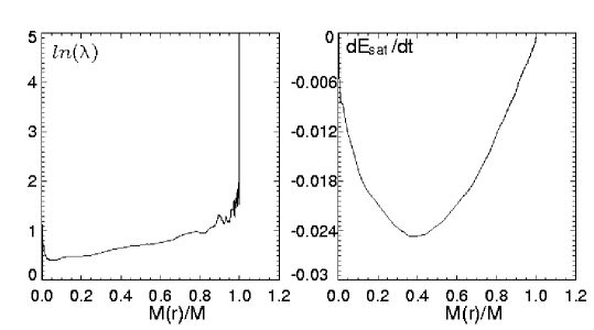
Figure 1: Numerical measurement of the Coulomb logarithm (left) and of the satellite energy loss by dynamical friction (right) for run $A_{1}$ (characterized by $M_{s}/M=0.1$, $R_{s}/R=0.1$, $t_{fall}/t_{cr}=48.125$). The quantities are plotted against a Lagrangian radial coordinate in the same format as in the paper by Bontekoe & van Albada (1987).

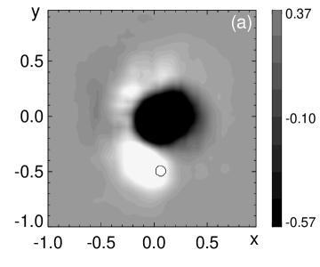
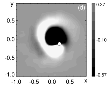
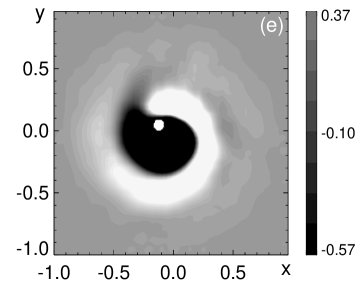
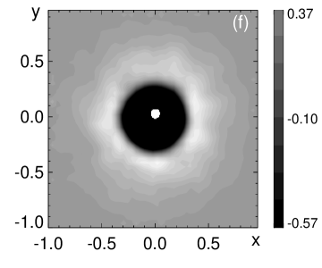
Figure 2: Six frames describing the equatorial density response $\rho_{1}=\rho-\rho_{0}$ of the galaxy to the infalling satellite for run $A_{1}$. The density wakes are portrayed at time $t/t_{cr}=$ (a) 38.5, (b) 39.875, (c) 41.25, (d) 42.625, (e) 44, and (f) 53.625. The white circle denotes the location of the satellite.

Figure 3: For each frame of Fig. 2 we illustrate in detail the monopole $(l=0)$ and the dipole $(l=1)$ contributions to the density wake in the galaxy (the various curves represent the coefficients $A_{10}$, $A_{11}$, $A_{00}$, and $B_{11}$ defined in the text; see Sect. 4.3).

Figure 4: For run $A_{1}$ we plot the mean azimuthal velocity of the galaxy measured on the equatorial plane at three different times; the rotation induced by the angular momentum exchange with the infalling satellite is approximately that of a solid body. As usual, time is measured in units of $t_{cr}$.

Figure 5: For run $A_{1}$ we plot two othogonal equatorial cuts of the anisotropy distribution generated in the galaxy by the infalling satellite at time $t=53.625\leavevmode\nobreak\ t_{cr}$, after the satellite has reached the center.

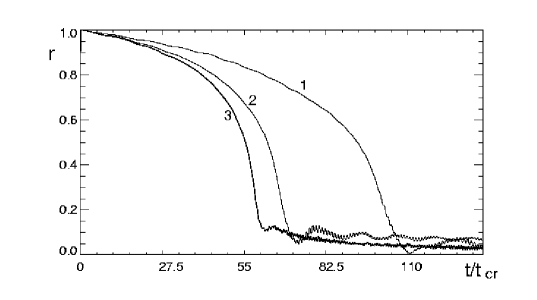
Figure 6: The curves illustrate the orbital decay process for the satellite for three different runs ($A_{6}$, $A_{8}$, and $A_{9}$, labeled as 1, 2, and 3 respectively) characterized by different spatial size of the infalling satellite ($R_{s}=0.1,\leavevmode\nobreak\ 0.05,\leavevmode\nobreak\ 0.025\leavevmode\nobreak\ R$; $M_{s}/M=0.05$).

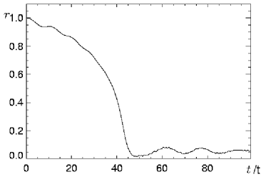
Figure 7: Left: The density distribution change induced in the galaxy by the infall of the satellite (run $A_{1}$). The thick upper curve (1) represents the initial distribution, while the thin lower curve (2) is associated with the final state. Right: Orbital decay for run $A_{1}$ (cf. Fig. 2) as in Fig. 6.

5.2 The case of many fragments

5.2.1 Case I

For various runs of type $B$ and $C$ we have checked that the total energy conservation generally holds, over a period of $\approx 100\leavevmode\nobreak\ t_{cr}$, to better than one part over 500. Yet, it is difficult to estimate the impact of dynamical friction on the galaxy evolution, because secular effects are masked by effects related to the initial lack of equilibrium. From this class of numerical experiments we have obtained the following results:

• We have observed a process of shell diffusion, which is a collective effect qualitatively different from what might have been imagined by simply superposing the effects of orbital decay of the individual fragments. The phenomenon persists, presumably via interaction with the wakes induced by the fragments in the galaxy, even when the direct fragment-fragment interaction is turned off. Sharp coherent oscillations are noted at early times; they are recognized as epicyclic oscillations generated by our choice of initial velocities for the fragments. We have also performed tests on the process of shell diffusion and oscillations on the basis of 400 fragments initially located close to $r=0.6\leavevmode\nobreak\ R$.

• We have noted systematic changes of the galaxy density distribution. The general trend emerging from the simulations is that significant peaking of the density distribution may occur, provided the initial radius of one shell of fragments is well inside the galaxy. However, much of the change is apparently associated with the initial lack of equilibrium.

• The process of density profile modification is not accompanied by the development of significant pressure anisotropy.

In conclusion, simulations of Case I turn out to be of little direct use for the main objectives of our project. However, they are extremely useful and instructive, because they demonstrate that, in order to properly single out slow relaxation processes, one has to be very careful about the choice of initial conditions and, in particular, because they provide concrete examples of some misleading effects that can occur as a result of the use of improper models.

5.2.2 Case II

The use of the smoother initialization described as case II in Sect. 3.2.2 leads to runs where the secular effects associated with the granularity of the fragment population are more convincingly identified. The orbital decay of the fragments is illustrated in Fig. 8, where we also show for comparison a parallel run where the shell is treated as collisionless. The interaction which generates dynamical friction of the galaxy on the fragments is responsible for the slow, but systematic, development of a tangential bias in the pressure tensor, as illustrated in Fig. 9 and for an overall change in the density profile of the galaxy (see Fig. 10).

The check against the collisionless run is worth a special digression. In order to diagnose the collisionality present in our system better, we have performed the following test. We have studied the correlation between single particle energy (for the particles simulating the galaxy) at two different times. If the simulation is truly collisionless, the single particle energy $E_{p}=mv^{2}/2+m\Phi(r)$, where $\Phi(r)$ is the mean field potential, should be strictly conserved. Indeed, by means of a plot similar to the lower right frame of Fig. 8, we have checked that for the run illustrated by the lower left frame of Fig. 8 more than $90\%$ of the particles have an energy correlation such that $|[E_{p}(t=118\leavevmode\nobreak\ t_{cr})-E_{p}(t=14\leavevmode\nobreak\ t_{cr})]/E_{p}(t=14\leavevmode\nobreak\ t_{cr})|<0.06$. In turn, for run $BS_{2}$, otherwise similar, but characterized by the presence of 100 fragments, a similar level of correlation for single particle energy (at 6 %) is preserved within the same time interval only by 50 % of the particles; the lower right frame of Fig. 8 thus illustrates the “damage” associated with dynamical friction.

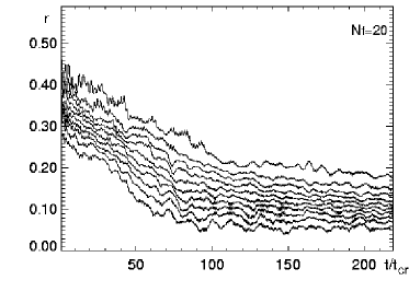
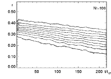
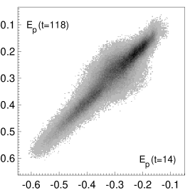
Figure 8: The fall of a shell of fragments towards the galaxy center, for the case of $N_{f}=20$ (left frame on the top, run $BS_{1}$) and for $N_{f}=100$ (right frame on the top, run $BS_{2}$). For comparison, the left frame at the bottom describes the time evolution of a collisionless shell (a run with $N_{f}=5\cdot 10^{4}$). Displayed lines represent 5, 15, 25, 35, 45, 55, 65, 75, 85, and 95 % of the shell mass. The right frame at the bottom displays, for run $BS_{2}$, the correlation between single particle energy at time $t=14\leavevmode\nobreak\ t_{cr}$ and energy at time $t=118\leavevmode\nobreak\ t_{cr}$, showing the effects of scattering associated with dynamical friction; units for energy are those indicated in Sect. 4.1.

Figure 9: The development of pressure anisotropy in the galaxy as a result of the interaction with a shell of fragments dragged in towards the galaxy center, for the case of $N_{f}=20$ (left frame, run $BS_{1}$) and for $N_{f}=100$ (right frame, run $BS_{2}$). The dashed curves represent the evolving value of $K_{T}/2$, where $K_{T}$ is the total kinetic energy associated with the star motions in the tangential directions; the solid curve represents the evolving value of $K_{r}$, the total kinetic energy associated with the star motions in the radial direction.

5.2.3 Case III

The even smoother procedure of case III leads to slower orbital decays, as illustrated in the lower frames of Fig. 11. For this type of simulations, the initial distribution of fragment orbits replicates the isotropic star distribution of the underlying galaxy. Because of dynamical friction, the fragment orbits are subject to a slow process of circularization, as illustrated in the upper frames of Fig. 11.

Figure 10: The change in density profile for the galaxy as a result of the interaction with a shell of fragments dragged in towards the galaxy center, for the case of $N_{f}=20$ (run $BS_{1}$). The thicker curve (1) represents the initial density profile, the thinner (2) gives the final profile.

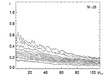
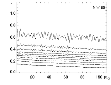
Figure 11: The effects of dynamical friction on a shell of fragments created out of the initial distribution function (case III of Sect. 3). The lower frames show the general decay of orbits of the fragments for the case $N_{f}=20$ (run $BT_{3}$) and $N_{f}=100$ (run $BT_{4}$); displayed lines represent 5, 15, 25, 35, 45, 55, 65, 75, 85, and 95 % of the shell mass. For the two runs, the upper frames show the corresponding effect of circularization of orbits; here the histograms record the number of fragments (crosses represent initial conditions, open circles the conditions at the end of the run) with orbit aspect ratio above $R_{\rm min}/R_{\rm max}$, where $R_{\rm min}$ and $R_{\rm max}$ are consecutive minimum and maximum radii attained by a fragment along its orbit.

Figure 12: The energies associated with the system of minisatellites (left frame) and measurement of the Coulomb logarithm $<ln(\lambda)>=\sum_{j=1}^{j=N_{f}}ln(\lambda)/N_{f}$ (right frame) (run $BS_{2}$).

For each of the fragments that are involved in the simulation described as Case II, we can repeat the analysis that has led to the measurement of the Coulomb logarithm from the study of the decay of the orbit of a single satellite. For example, for run $BS_{2}$ we have 100 independent such determinations. In Fig. 12 we record, for run $BS_{2}$ a measurement of an average value of the Coulomb logarithm. We note that the fact that the value of the Coulomb logarithm thus determined remains of the same order of magnitude as that obtained in Fig. 1 proves that the classical expression for the effects of dynamical friction captures the correct scaling with respect to the mass of the object subject to friction.

6 Discussion and conclusions

In this paper we have set up a numerical laboratory for the study of dynamical friction in inhomogeneous quasi-spherical galaxies and made several experiments that have elucidated the physical mechanisms that participate in the process.

The general character of the simulations presented here is distinctly different from that adopted in previous studies in this general research area, because we have addressed a physical scenario in which the slow collapse induced by dynamical friction approximately preserves the spherical symmetry present initially. This configuration is inspired by the astrophysical problem of studying the evolution of a spherical galaxy in the presence of a substantial globular cluster system or as a result of the capture of a large set of mini-satellites dragged in along random directions.

From the theoretical point of view, the framework adopted here has an important advantage with respect to the traditional case of the study of the decay of the orbit of a single satellite, because it allows us to run smoother simulations that are basically free from other effects unrelated to dynamical friction, such as those associated with lack of equilibrium in the initial configuration.

In the past, most of the attention has been focused on the effect of the host galaxy on the object subject to dynamical friction. Here, we have been able not only to test the adequacy of the classical formulae of dynamical friction (derived for ideal homogeneous models) in the inhomogeneous galaxy environment, but also to measure the evolution of the density and pressure tensor profiles in the galaxy induced by the presence of friction processes on a minority population of heavier particles. We have made quantitative tests that convince us that we are detecting genuine effects associated with secular evolution.

6.1 Plans for future investigations

Starting from the encouraging quantitative results obtained in this paper, there are now two major issues that we would like to address in investigations planned for the near future, which appear to be approachable by the use of the numerical laboratory developed here:

• In this paper we have limited our study to the presence of one or two shells of heavy particles, so as to probe the reaction of the galaxy distribution function in a controlled way and to test whether the interaction involved can be described as “local”. The first immediate objective that we have in mind is to devise a set of more realistic simulations, able to represent the distribution of the globular cluster system in galaxies better.

• So far we have limited our discussion to the study of the orbital decay in an $n=3$ polytropic, isotropic galaxy model. Now we would like to test systematically the process of slow collapse induced by dynamical friction as a function of the concentration properties of the equilibrium model, for the case of more realistic galaxy models.

- (1) Barnes, J., & Hut, P. 1986, Nature, 324, 446
- (2) Bertin, G., Pegoraro, F., Rubini, F., & Vesperini, E. 1994, ApJ, 434, 94 [BPRV94]
- (3) Bertin, G., & Trenti, M. 2003, ApJ, 584, 729
- (4) Bonnor, W.B. 1956, MNRAS, 116, 351
- (5) Bontekoe, Tj. R. 1988, Ph.D. Thesis, Groningen University, Groningen
- (6) Bontekoe, Tj.R., & van Albada, T.S. 1987, MNRAS, 224, 349
- (7) Chandrasekhar, S. 1943, ApJ, 97, 251
- (8) Cipollina, M., & Bertin, G. 1994, A&A, 288, 43
- (9) Colpi, M. 1998, ApJ, 502, 167
- (10) Colpi, M., & Pallavicini, A. 1998, ApJ, 502, 150
- (11) Colpi, M., Mayer, L., & Governato, F. 1999, ApJ, 525, 720
- (12) Cora, S.A., Muzzio, J.C., & Vergne, M.M. 1997, MNRAS, 289, 253
- (13) Cora, S.A., Vergne, M.M., & Muzzio, J.C. 2001, ApJ, 564, 165
- (14) Fridman, A.M., & Polyachenko, V.L. 1984, Physics of Gravitating Systems, (Springer-Verlag, Berlin)
- (15) Hernquist, L., & Weinberg, M.D. 1989, MNRAS, 238, 407
- (16) Hohl, F. 1973, ApJ, 184, 353
- (17) Huang, S., Dubinski, J., & Carlberg, R.G. 1993, ApJ, 404, 73
- (18) Lotz, J.M. et al. 2001, ApJ, 552, 572
- (19) Lynden-Bell, D., & Wood, R. 1968, MNRAS, 138, 495
- (20) Maoz, E. 1993, MNRAS, 263, 75
- (21) Milosavljevich, M., & Merritt, D. 2001, ApJ, 563, 34
- (22) Nelson, R.W., & Tremaine, S. 1999, MNRAS, 306, 1
- (23) Palmer, P.L. 1994, Stability of collisionless stellar systems, (Kluwer, Dordrecht)
- (24) Palmer, P.L., & Papaloizou, J. 1985, MNRAS, 215, 691
- (25) Pfenniger, D. 1986, A&A, 165, 74
- (26) Press, W.H., Teukolsky, S.A., Vetterling, W.T., & Flannery, B.P. 1992, Numerical Recipes, Second Edition (Cambridge University Press, Cambridge)
- (27) Prugniel, Ph., & Combes, F. 1992, A&A, 259, 25
- (28) Quinlan, G.D. & Hernquist, L. 1997, New Astron., 2, 533
- (29) Séguin, P., & Dupraz, C. 1994, A&A, 290, 709
- (30) Séguin, P., & Dupraz, C. 1996, A&A, 310, 757
- (31) Spitzer, L. 1987, Dynamical Evolution of Globular Clusters, (Princeton University Press, Princeton)
- (32) Springel, V., Yoshida, N., & White, S. D. M. 2001, New Astronomy, 6, 79
- (33) Tremaine, S., Ostriker, J.P., & Spitzer, L. 1975, ApJ, 196, 407
- (34) van Albada, T.S. 1982, MNRAS, 201, 939
- (35) van Albada, T.S., & van Gorkom, J.H. 1977, A&A, 54, 121
- (36) Vesperini, E., & Weinberg, M.D. 2000, ApJ, 534, 598
- (37) Weinberg, M.D. 1986, ApJ, 300, 93
- (38) Weinberg, M.D. 1989, MNRAS, 239, 549
- (39) Zaritsky, D., & White, S.D.M. 1988, MNRAS, 235, 289