Halo Substructure and the Power Spectrum

Abstract

We present a semi-analytic model to investigate the merger history, destruction rate, and survival probability of substructure in hierarchically formed dark matter halos, and use it to study the substructure content of halos as a function of input primordial power spectrum. For a standard cold dark matter “concordance” cosmology ($\Lambda$CDM; $n=1$, $\sigma_{8}=0.95$) we successfully reproduce the subhalo velocity function and radial distribution profile seen in N-body simulations, and determine that the rate of merging and disruption peaks $\sim 10-12$ Gyr in the past for Milky Way-like halos, while surviving substructures are typically accreted within the last $\sim 0-8$ Gyr. We explore power spectra with normalizations and spectral “tilts” spanning the ranges $\sigma_{8}\simeq 1-0.65$ and $n\simeq 1-0.8$, and include a “running-index” model with ${\rm d}n/{\rm d}\ln k=-0.03$ similar to the best-fit model discussed in the first-year WMAP report. We investigate spectra with truncated small-scale power, including a broken-scale inflation model and three warm dark matter cases with $m_{\rm W}=0.75-3.0$ keV.

We find that the mass fraction in substructure is relatively insensitive to the tilt and overall normalization of the primordial power spectrum. All of the CDM-type models yield projected substructure mass fractions that are consistent with, but on the low side, of published estimates from strong lens systems: $f_{9}=0.4-1.5\%$ ($64$ percentile), for subhalos $<10^{9}$ M_⊙ within projected cylinders of radius $r<10$ kpc. Truncated models produce significantly smaller fractions, $f_{9}=0.02-0.2\%$ for $m_{\rm W}\simeq 1$ keV, and are disfavored by lensing estimates of substructure. This suggests that lensing and similar probes can provide a robust test of the CDM paradigm and a powerful constraint on broken-scale inflation/warm particle masses, including masses larger than the $\sim 1$ keV upper limits of previous studies. We compare our predicted subhalo velocity functions to the dwarf satellite population of the Milky Way. Assuming dwarfs have isotropic velocity dispersions, we find that the standard $n=1$ model over-predicts the number of Milky Way satellites at $V_{\rm max}\lower 2.58334pt\vbox{\hbox{$\buildrel\textstyle<\over{\sim}\ $}}35\textrm{ km s}^{-1}$, as expected. Models with less small-scale power do better because subhalos are less concentrated and the mapping between observed velocity dispersion and halo $V_{\rm max}$ is significantly altered. The running-index model, or a fixed tilt with $\sigma_{8}\sim 0.75$, can account for the local dwarfs without the need for differential feedback (for $V_{\rm max}\lower 2.58334pt\vbox{\hbox{$\buildrel\textstyle>\over{\sim}\ $}}20\textrm{ km s}^{-1}$); however, these comparisons depend sensitively on the assumption of isotropic velocities in satellite galaxies.

1 INTRODUCTION

In the standard cosmological model of structure formation ($\Lambda$CDM), the Universe is dominated by cold, collisionless dark matter (CDM), made flat by a cosmological constant ($\Lambda$), and endowed with initial density perturbations via quantum fluctuations during inflation. The $\Lambda$CDM  model with $\Omega_{\rm M}=1-\Omega_{\rm\Lambda}=0.3$, $h\approx 0.7$, and a scale-invariant spectrum of primordial perturbations ($P(k)\propto k^{n}$, $n=1$, $\sigma_{8}\sim 0.9$) is remarkably successful at reproducing a plethora of large-scale observations (e.g., Spergel et al. 2003; Percival et al. 2002). In contrast, several small-scale observations have proven more difficult to explain. Galaxy densities and concentrations appear to be much lower than what is predicted for the standard ($n=1$) $\Lambda$CDM model (e.g., Debattista & Sellwood 2000; Côte, Carignan, & Freeman 2000; Borriello & Salucci 2000; Binney & Evans 2001; Keeton 2001; van den Bosch & Swaters 2001; Marchesini et al. 2002; Swaters et al. 2003; McGaugh, Barker, & de Blok 2003; van den Bosch, Mo, & Yang 2003), and the Local Group dwarf galaxy count is significantly below what might naively be expected from the substructure content of $\Lambda$CDM halos (Klypin et al. 1999a, K99 hereafter; Moore et al. 1999a). In Zentner & Bullock (2002, hereafter ZB02), we showed that the central densities of $\Lambda$CDM dark matter halos can be brought into reasonable agreement with the rotation curves of dark matter-dominated galaxies by reducing galactic-scale fluctuations in the initial power spectrum ($\sigma_{8}\sim 0.75$ and $n\sim 0.9$ is a good match; see Alam, Bullock, & Weinberg 2002, hereafter ABW; McGaugh et al. 2003; van den Bosch et al. 2003). The present paper is an extension of this work. We explore how changes in the initial power spectrum affect the substructure content of $\Lambda$CDM halos, test our findings against attempts to measure the substructure mass fraction via gravitational lensing, and relate our results to the question of the abundance of dwarf satellites in the Local Group.

It is straightforward to see why CDM halos are expected to play host to a large number of distinct, bound substructures, or “subhalos.” In the modern picture of hierarchical structure formation (White & Rees 1978; Blumenthal et al. 1984; Kauffmann, White, & Guiderdoni 1993) low-mass systems collapse early and merge to form larger systems over time. Small halos collapse at high redshift, when the universe is very dense, so their central densities are correspondingly high. When these halos merge into larger hosts, their high densities allow them to resist the strong tidal forces that act to destroy them. While gravitational interactions do serve to unbind most of mass associated with merged progenitors, a significant fraction of these small halos survive as distinct substructure.

Our understanding of this process has increased dramatically in the last five years thanks to remarkable advances in N-body techniques that allow the high force and mass resolution necessary to study substructure in detail (Ghigna et al. 1998, 2000; Kravtsov 1999; K99; Klypin et al. 1999b; Kolatt et al. 1999; Moore et al. 1999a,b; Font et al. 2001; Stoehr et al. 2002). For $n=1$, $\Lambda$CDM and CDM simulations, the total mass fraction bound up in substructure is measured at $f\sim 5-15\%$ (Ghigna et al. 1998, Klypin et al. 1999b), with a significant portion contributed by the most massive subsystems, $dN/dM\propto M^{-s}$, $s\approx 1.7$. The substructure content of halos seems to be roughly self-similar when subhalo mass is scaled by the host halo mass (Moore et al. 1999a) and the subhalo count is observed to decline at the host halo center, where tidal forces are strongest (Ghigna et al. 1998; Colín et al. 2000b; Chen, Kravtsov, & Keeton 2003).

Unfortunately, studies of substructure using N-body simulations suffer from issues of numerical resolution. Simulations with the capability to resolve substructure are computationally expensive. They cannot be used to study the implications of many unknown input parameters and cannot attain both the resolution and the statistics needed to confront observational data on substructure that appear to be on the horizon. Even state of the art simulations face difficulties in the centers of halos where “overmerging” may be a problem (e.g., Chen et al. 2003; Klypin et al. 1999b) and measurements of the substructure fraction via lensing are highly sensitive to these uncertain, central regions. Our goal is to present and apply a semi-analytic model that suffers from no inherent resolution effects, and is based on the processes that were observed to govern substructure populations in past N-body simulations. This kind of model can generate statistically significant predictions for a variety of inputs quickly and can be used to guide expectations for the next generation of N-body simulations. Conversely, this model represents in many ways an extrapolation of N-body results into unexplored domains and it is imperative that our results be tested by future numerical studies. In the present paper, we aim to explore the effect of the power spectrum on the population of surviving subhalos, but in principle these methods are suitable for testing substructure ramifications for a variety of cosmological inputs.

One of the main motivations for this work comes from simulation results that indicate that galaxy-sized CDM halos play host to hundreds of subhalos with maximum circular velocities in the range $10\textrm{ km s}^{-1}$ $\buildrel\textstyle<\over{\sim}\$ $V_{\rm max}$ $\buildrel\textstyle<\over{\sim}\$ $30$ $\textrm{ km s}^{-1}$. The Milky Way, as a comparative example, hosts only $11$ dwarf satellites of similar size. This “dwarf satellite problem” specifically refers to the gross mismatch between the predicted number of $\Lambda$CDM subhalos and the count of satellite galaxies in the Local Group (K99; Moore et al. 1999a; Font et al. 2001; see also Kauffmann et al. 1993, who indicated that there may be a problem using analytic arguments). The dwarf satellite problem and other small-scale issues led many authors to consider modifications to the standard framework. If the dark matter were “warm” (Pagels & Primack 1982; Colombi, Dodelson, & Widrow 1996; Hogan & Dalcanton 2000; Colín et al. 2000a; Bode, Ostriker, & Turok 2001; Lin et al. 2001; Knebe et al. 2002) or if the primordial power spectrum were sharply truncated on small scales (Starobinsky 1992; Kamionkowski & Liddle 2000) then subgalactic-scale problems may be allayed without vitiating the overall success of $\Lambda$CDM on large scales. Another possibility is that CDM substructure is abundant in all galaxy halos, but that most low-mass systems are simply devoid of stars. An intermediate solution may involve a simple modification of the assumed primordial spectrum of density perturbations that gradually lowers power on galactic scales relative to the horizon, e.g., via tilting the power spectrum.

Probing models with low galactic-scale power is motivated not only by the small-scale crises facing standard $\Lambda$CDM but also by more direct probes of the power spectrum. While many analyses continue to measure “high” values for $\sigma_{8}\sim 1$ (Van Waerbeke et al. 2002; Komatsu & Seljak 2002; Bahcall & Bode 2003; where $\sigma_{8}$ is the linear, rms fluctuation amplitude on a length scale of 8 h^-1 Mpc ), numerous recent studies relying on similar techniques, advocate rather “low” values of $\sigma_{8}\sim 0.7-0.8$ (Jarvis et al. 2003; Bahcall et al. 2003; Schuecker et al 2003; Pierpaoli et al. 2003; Viana et al. 2002; Brown et al. 2002; Allen et al. 2002; Hamana et al. 2002; Melchiorri & Silk 2002; Borgani et al. 2001). Similarly, the Ly-$\alpha$ forest measurements of the power spectrum are consistent with reduced galactic-scale power (Croft et al. 1998; McDonald et al. 2000; Croft et al. 2002). Set against the normalization of fluctuations on large scales implied by the Cosmic Background Explorer (COBE) measurements of cosmic microwave background (CMB) anisotropy (Bennett et al. 1994), these data suggest that the initial power spectrum may be tilted to favor large scales with $n<1$.

The recent analysis of the Wilkinson Microwave Anisotropy Probe (WMAP) measurements of CMB anisotropy presented by Spergel et al. (2003; see also Verde et al. 2003; Peiris et al. 2003) returns a best-fit spectral index to a pure power law primordial spectrum of $n=0.99\pm 0.04$ when only the WMAP data are considered. However, when data from smaller scale CMB experiments, the 2dF Galaxy Redshift Survey, and the Ly-$\alpha$ forest are included, the analysis favors a mild tilt, $n=0.96\pm 0.02$. Interestingly, all of the data sets together yield a better fit if the index is allowed to run: the WMAP team find ${\rm d}n/\rm{d}\ln k=-0.031^{+0.016}_{-0.017}$. This result is consistent with no running at $\sim 2\sigma$, and the statistical significance is further weakened when additional uncertainties in the mean flux decrement in the Ly-$\alpha$ forest are considered (Seljak, McDonald, and Makarov 2003; Croft et al. 2002), yet such a model certainly seems worth investigating, especially in light of the small-scale difficulties it may help to alleviate.

We explicitly show how models with reduced small-scale power are expected to help the halo density problem in Figure 1, which is an updated version of Figure 5 in ZB02. Here, we compare the densities of standard $n=1$ halos to galaxy rotation curve data (see ZB02 for details) along with expectations for the running-index (RI) model favored by WMAP and several other models we explore in the following sections. Galaxy and halo densities (vertical axis) are evaluated at the radius where the rotation curve falls to half its maximum value and expressed in units of the critical density ($\Delta_{V/2}$, as defined in ABW). Clearly, the data favor low small-scale power relative to the standard $n=1$ case.

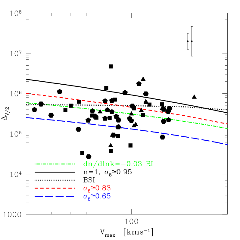
Figure 1: Galaxy central densities. The symbols show the mean density (relative to the critical density) within the radius where each rotation curve falls to half of its maximum value, inferred from the measured rotation curves of several dark matter-dominated dwarf and low surface brightness galaxies (see ZB02 for details). The data are taken from de Blok, McGaugh, & Rubin (2001; triangles and hexagons), de Blok and Bosma (2002; squares), and Swaters (1999; pentagons). The lines show the theoretical expectation for several of the power spectra we describe in §3 and Table 1. The points with error bars in the upper right corner reflect the expected theoretical scatter in the density as inferred by Bullock et al. (2001, larger range) and Jing (2000, smaller range).

The possibility of discriminating between standard $\Lambda$CDM and several alternatives has inspired efforts to measure and quantify the substructure content of galactic halos. One method relies on studying tidal tails associated with known Galactic satellites (Johnston, Spergel, & Haydn 2002; Ibata et al. 2002a, 2002b; Mayer et al. 2002). Subhalos passing through cold tidal streams scatter stars away from their original orbits, and the signatures of these events may be detectable in the velocity data of future astrometric missions and several deep halo surveys that will soon be completed. Of particular interest for obtaining measurements in distant galaxies are studies that aim to detect substructure via flux ratio anomalies in strong gravitational lenses (Moore et al. 1999a; Metcalf & Madau 2001; Metcalf & Zhao 2002; Bradač et al. 2002). Using a sample of seven four-image radio lenses, Dalal & Kochanek (2001, DK01 hereafter) estimated a mass fraction of $f=0.006-0.07$ (90% confidence level) bound up in substructure less massive than $\sim 10^{8}-10^{10}$ M_⊙, in line with the rough expectations of CDM. While measurements of this kind are susceptible to potential degeneracies with the adopted smooth lens model and other uncertainties, they are encouraging and serve as prime motivators for this work (see Kochanek & Dalal 2003). In addition, new observational techniques that focus on astrometric features (Metcalf 2002), and particularly spectroscopic studies of strong lens systems (Moustakas & Metcalf 2003), promise to hone in on the masses of the subclumps responsible for the lensing signals.

If the Milky Way really is surrounded by a large number of dark subhalos, the dwarf satellite problem serves as a conspicuous reminder that feedback plays an important role in hierarchical galaxy formation. Of course, the need for feedback in small systems has been generally recognized for some time (e.g., White & Rees 1978). Supernova blow-out likely plays a role in regulating star formation if CDM is the correct theory (Dekel & Silk 1986; Kauffmann et al. 1993; Cole et al. 1994; Somerville & Primack 1999); however, supernova winds do not naturally suggest a sharp discrepancy at $\sim 30\textrm{ km s}^{-1}$, nor do they explain why some halos of this size should have stars while most have none at all. It seems more likely that supernovae play an important role in setting scaling relations in slightly larger galaxies ($V_{\rm max}\sim 100\textrm{ km s}^{-1}$; Dekel & Woo 2002; but see Mac Low & Ferrara 1999). Perhaps a more natural feedback source on satellite galaxy scales is the ionizing background, which should suppress galaxy formation in halos with $V_{\rm max}\lower 2.58334pt\vbox{\hbox{$\buildrel\textstyle<\over{\sim}\ $}}30\textrm{ km s}^{-1}$ (Rees 1986; Efstathiou 1992; Kauffmann et al. 1993; Shapiro, Giroux, & Babul 1994; Thoul & Weinberg 1996; Quinn, Katz, & Efstathiou 1996; Gnedin 2000). Bullock, Kravtsov, & Weinberg (2000, BKW hereafter) suggested that dwarf galaxies may be associated with small halos that collapsed before the epoch of reionization, and though the method used by BKW to estimate dwarf luminosities was crude, more sophisticated models have since led to similar conclusions (Chiu, Gnedin, & Ostriker 2001; Somerville 2002; Benson et al. 2002). For the smallest systems, $V_{\rm max}\lower 2.58334pt\vbox{\hbox{$\buildrel\textstyle<\over{\sim}\ $}}10-20\textrm{ km s}^{-1}$, the ionizing background likely stops star formation altogether by photo-evaporating gas in halos, even after they have collapsed (Barkana & Loeb 1999; Shaviv & Dekel 2003).

Precisely what can be learned about galaxy formation and/or cosmology by counting dwarf satellites depends upon our expectations for the density profiles of their host halos. To count satellites of a given maximum circular velocity, we must infer a halo $V_{\rm max}$ using the observed central velocity dispersion $\sigma_{\star}$, and the mapping between these two quantities depends sensitively on the structure of each satellite’s dark matter halo. This point was first emphasized by S. D. M. White at the Summer $2000$ Institute for Theoretical Physics Conference on Galaxy Formation and Evolution. Standard $\Lambda$CDM halos with $V_{\rm max}\sim 30\textrm{ km s}^{-1}$ are expected to be very concentrated (Colín et al. 2000a; Bullock et al. 2001), with their rotation curves peaking at $r_{\rm max}\sim 1$ kpc, so the multiplicative factor that converts a $\sim 1$ kpc velocity dispersion measurement to halo $V_{\rm max}$ is fairly modest: $V_{\rm max}\sim\sqrt{3}\sigma_{\star}$ (K99). However, as we discuss in §4, the appropriate conversion is cosmology-dependent because models with later structure formation tend to produce halos with more slowly rising rotation curves. If a dwarf galaxy sits in a halo with a slowly rising rotation curve that peaks at $r_{\rm max}\gg$ a few kpc, the conversion factor, and thus $V_{\rm max}$, can be significantly larger. Shifts of this kind in the “observed” velocity function change the implied velocity (or mass) scale of discrepancy, and influence our ideas about the type of feedback that gives rise to the mismatch.

Hayashi et al. (2003, H03 hereafter) and Stoehr et al. (2002, S02 hereafter) suggested that substructure halos experience significant mass redistribution in their centers as a result of tidal interactions and that they are therefore less concentrated than comparable halos in the field. They argue that when this is taken into account, the dwarf satellite mismatch sets in at $V_{\rm max}\sim 20\textrm{ km s}^{-1}$, and that the transition is sudden — below this scale all halos are devoid of observable galaxies. While these conclusions have yet to be confirmed and are dependent upon subhalo merger histories and the isotropy of dwarf velocity dispersions, they highlight the need to refine our predictions about halo substructure. They also motivate us to explore how minor changes in cosmological parameters can influence our interpretation of the dwarf satellite problem.

In the remainder of this paper we present our study of CDM substructure. In §2, we describe our semi-analytic model, provide some illustrative examples, and compare our results for standard $\Lambda$CDM to previous N-body results. In §3, we briefly describe the input power spectra that serve as the basis for this study. In §4, we present our results on subhalo mass functions and velocity functions. We make predictions aimed at measuring substructure mass fractions via gravitational lensing and address the dwarf satellite problem in light of some of our findings in this section. In §5 we discuss some shortcomings of our model and how they might be improved in future work. In §6 we summarize our work and draw conclusions from our results. In this study we vary only the power spectrum and work within the context of the so-called “concordance” cosmological model with $\Omega_{\rm M}=0.3$, $\Omega_{\rm\Lambda}=0.7$, $h=0.72$, and $\Omega_{\rm B}h^{2}=0.02$ (e.g., Turner 2002; Spergel et al. 2003).

2 MODELING HALO SUBSTRUCTURE

In order to determine the substructure properties of a dark matter halo we must model its mass accretion history as well as the orbital evolution of the subsystems once they are accreted. For the first step, we rely on the the extended Press-Schechter (EPS) formalism to create merger histories for each host system. We give a brief description of our EPS merger trees in §2.1. In §2.2 we discuss our model for the density structure of accreted halos and the host system and in §2.3 we describe our method for following the orbital evolution of each merged system. We show tests and examples of this model in §2.4.

2.1 Merger Histories

We track diffuse mass accretion and satellite halo acquisition of host systems by constructing merger histories using the EPS method (Bond et al. 1991; Lacey & Cole 1993, LC93 hereafter). In particular, we employ the merger tree algorithm of Somerville and Kolatt (1999, hereafter SK99). This allows us to generate a list of the masses and accretion redshifts of all subhalos greater than a given threshold mass that merged to form the host halo. We describe the method briefly here, and encourage the interested reader to consult LC93 and SK99 for further details.

A merger tree that reproduces many of the results of N-body simulations can be constructed using only the linear power spectrum. For convenience, we express this in terms of $\sigma(M)$, the rms fluctuation amplitude on mass scale $M$ at $z=0$. As in LC93, let $S(M)\equiv\sigma^{2}(M)$, $\Delta S\equiv S(M)-S(M+\Delta M)$, $w(t)\equiv\delta_{\rm c}(t)$, and $\delta w\equiv w(t)-w(t+\Delta t)$. Here $\delta_{\rm c}(t)$ is the linear overdensity for collapse at time t, associated with our choice of cosmology (see LC93 or White 1996). The probability that a halo of mass $M$, at time $t$, accreted an amount of mass associated with a step of $\Delta S$, in a given time step implied by $\delta w$ is

$$P(\Delta S,\delta w)\textrm{d}(\Delta S)=\frac{\delta w}{\sqrt{2\pi}\Delta S^{3/2}}\exp\Bigg{[}\frac{-(\delta w)^{2}}{2\Delta S}\Bigg{]}\textrm{d}(\Delta S).$$ (1)

Merger histories are constructed by starting at a chosen redshift and halo mass and stepping back in time with an appropriate time step. If the minimum mass of a progenitor that we wish to track is $M_{\rm min}$, then SK99 tell us that each time step must be small in order to reproduce the conditional mass functions of EPS theory: $\delta w\lower 2.58334pt\vbox{\hbox{$\buildrel\textstyle<\over{\sim}\ $}}\sqrt{M_{\rm min}(\textrm{d}S(M)/\textrm{d}M)}$.

We build merger trees by selecting progenitors at each time step according to equation (1) and treating events with $\Delta M<M_{\rm min}$ as diffuse mass accretion. At each step, we identify the most massive progenitor with the host halo and all less massive progenitors with accreted subhalos and we continue this process until the host mass falls below $M_{\rm min}$. In practice, we use a slightly modified version of the SK99 scheme. At each stage we demand that the number of progenitor halos in the mass range we consider be close to the mean value. As discussed in BKW, this modification considerably improves the agreement between the analytically predicted progenitor distribution and the numerically generated progenitor distribution. In what follows we set $M_{\rm min}=10^{5}$ M_⊙. Our fiducial, z=0 host mass is $1.4\times 10^{12}$ M_⊙, but we vary these choices in order test sensitivity to the host mass and redshift.

2.2 Halo Density Structure

Whether a merged system survives or is destroyed depends on the density structure of the subhalo and on the gravitational potential of the host system. Therefore, it is worthwhile to describe our assumptions about CDM density profiles in some detail. The size of a virialized dark matter halo can be quantified in terms of its virial mass $M_{\rm vir}$, or equivalently its virial radius $R_{\rm vir}$, or virial velocity $V_{\rm vir}^{2}\equiv GM_{\rm vir}/R_{\rm vir}$. The virial radius of a halo is defined as the radius within which the mean density is equal to the virial overdensity $\Delta_{\rm vir}$, multiplied by the mean matter density of the Universe $\rho_{\rm M}$, so that $M_{\rm vir}=4\pi\rho_{\rm M}\Delta_{\rm vir}(z)R_{\rm vir}^{3}/3$. The virial overdensity $\Delta_{\rm vir}$, can be estimated using the spherical top-hat collapse approximation and is generally a function of $\Omega_{\rm M}$, $\Omega_{\rm\Lambda}$, and redshift (e.g., Eke, Navarro, & Frenk 1998). We compute $\Delta_{\rm vir}$ using the fitting function of Bryan & Norman (1998). In the cosmology considered here, $\Delta_{\rm vir}(z=0)\simeq 337$, and at high redshift $\Delta_{\rm vir}\rightarrow 178$, approaching the standard cold dark matter (i.e., $\Omega_{\rm M}=1$) value.

The gross structure of dark matter halos has been described by several analytic density profiles that have been proposed as good approximations to the results of high-resolution N-body simulations (Moore et al. 1999b; Power et al. 2003). In the interest of simplicity, we choose to model all halos with the density profile proposed by Navarro, Frenk, & White (1997; hereafter NFW):

$$\rho(r)=\frac{\rho_{\rm s}}{(r/r_{\rm s})(1+r/r_{\rm s})^{2}}.$$ (2)

For the NFW profile, the amount of mass contained within a radius r, is

$$M(<r)=M_{\rm vir}\frac{g(x)}{g(c_{\rm vir})}$$ (3)

where $x\equiv r/r_{\rm s}$, $g(y)\equiv\ln(1+y)-y/(1+y)$, and the concentration parameter is defined as $c_{\rm vir}\equiv R_{\rm vir}/r_{\rm s}$. Restating equation (3) in terms of a circular velocity profile yields $V_{c}^{2}(r)=V_{\rm vir}^{2}c_{\rm vir}g(x)/xg(c_{\rm vir})$. The maximum circular velocity occurs at a radius $r_{\rm max}\simeq 2.16r_{\rm s}$, with a value $V_{\rm max}^{2}\simeq 0.216V_{\rm vir}^{2}c_{\rm vir}/g(c_{\rm vir})$.

As a result of the study by Wechsler et al. (2002; W02 hereafter) and several precursors (e.g., Zaroubi and Hoffman 1993; NFW; Avila-Reese, Firmani, & Hernández 1998; Bullock et al. 2001, hereafter B01), we now understand that dark matter halo concentrations are determined almost exclusively by their mass assembly histories. The gross picture advocated by W02 is that the rate at which a halo accretes mass determines how close to the center of the host halo the accreted mass is deposited. When the mass accretion rate is high, near equal mass mergers are very likely, and dynamical friction acts to deposit mass deep into the interior of the host. After an early period of rapid mass accretion, the central densities of halos remain constant at a value proportional to the mean density of the Universe at the so-called “formation epoch” $z_{\rm c}$, defined as the redshift when the relative mass accretion rate was similar to the rate of universal expansion (see W02 for details). For typical halos, this formation epoch occurred at a time when halos were roughly $\sim 10-20\%$ of their final masses. Additionally, W02 found that the scale radius and central density of the best fit NFW profile remain practically constant after the initial phase of rapid accretion. After this time, the mass increase is slow, and as the virial radius of the halo grows, its concentration decreases as $c_{\rm vir}\propto(1+z)^{-1}$.

These results lend support to B01, who explained the observed trends with halo mass and redshift using a simple, semi-analytic model that we adopt in this study. In the B01 model, halo concentrations $c_{\rm vir}(M,z)$, depend only on the value of $\sigma(M)$ and the evolution of linear perturbations, $\delta(z)/\delta(z=0)$. Specifically, the density of a halo of mass $M$ is set by the density of the Universe at the time when systems of mass $\sim 0.01M$ were typically collapsing. The collapse epoch $z_{\rm c}$, is defined by $\sigma(0.01M)\equiv\delta_{\rm c}(z_{\rm c})$. Again, $\delta_{\rm c}(z)$ is the linear overdensity for collapse at redshift $z$. Central densities determined in this manner connect well to the findings of W02. Halo density structure is set at a time of rapid accretion, when progenitor masses typically were $M_{\rm prog}\sim 0.1M$. Most of the mass in a halo at any given time is set by accretion events with subhalos of mass $\sim 1/10$ the host halo mass (cf. §4). Thus the period of rapid mass accretion involves objects of mass $\sim 0.1M_{\rm prog}\sim 0.01M$, and it is the collapse times and densities of these constituents that set the central density of the mass $M$ halo.

The B01 model reproduces N-body results for $n=1$, $n=0.9$, and power-law CDM models (e.g., Colín et al. 2000b; B01) as well the WDM simulations of Colín et al. (2000a) and Avila-Reese et al. (2001). However, we stress that N-body tests were restricted to the mass range $\sim 10^{9}-10^{14}$ M_⊙ because of the limited dynamic range of numerical experiments. Nevertheless, we use the B01 model to compute concentrations for halos with masses $\ll 10^{9}$ M_⊙. Our results for $M\lower 2.58334pt\vbox{\hbox{$\buildrel\textstyle<\over{\sim}\ $}}10^{9}$ M_⊙ may be regarded as a “best-guess” extrapolation of N-body results.

Before proceeding, we mention an alternate prescription for assigning $c_{\rm vir}(M,z)$ proposed by Eke, Navarro, & Steinmetz (2001, ENS hereafter). ENS investigated the power spectrum dependence of the $c_{\rm vir}-M_{\rm vir}$ relation for several $\Lambda$CDM and WDM models. While the B01 and ENS recipes for $c_{\rm vir}(M,z)$ matched well for $\Lambda$CDM, the B01 model failed to reproduce the mass dependence seen in simulations by ENS for WDM halos with masses smaller than the “free-streaming” mass (see §3). The four WDM halos simulated by ENS with masses small enough to be appreciably affected by free-streaming all had $c_{\rm vir}$ values that were $\sim 2\sigma$ lower than the B01 model. Based on these data, ENS proposed a model in which halo collapse time depends not only on the amplitude of the power spectrum $\sigma(M)$, but on an effective overdensity amplitude, $\sigma_{\rm eff}\equiv-\sigma(M)\textrm{d}\ln\sigma(M)/\textrm{d}\ln M$. This results in a $c_{\rm vir}(M)$ relation that increases with mass for masses smaller than the truncation scale and decreases at larger masses as in $\Lambda$CDM. By defining an effective overdensity in this way, ENS were able to account for the low $c_{\rm vir}$ values observed in their WDM simulations and still reproduce the redshift and mass dependence seen in $\Lambda$CDM simulations. The slope of the $c_{\rm vir}$-$M_{\rm vir}$ of ENS is shallower than the slope predicted by the B01 relation, therefore the ENS model also leads to less concentrated halos at small mass ($M\lower 2.58334pt\vbox{\hbox{$\buildrel\textstyle<\over{\sim}\ $}}10^{10}$ M_⊙) even for identical input power spectra. This disparity grows larger when tilted and/or running spectra are considered, as in this paper.

Unfortunately, the ENS model cannot be applied in the WDM cases we explore because in these models $\sigma(M)$ is very flat on scales smaller than the free-streaming mass and the ENS model breaks down when $\textrm{d}\sigma(M)/\textrm{d}M$ becomes very small. In the ENS model, WDM halos smaller than $\sim 1\%$ of the free-streaming mass never collapse because $\sigma_{\rm eff}\ll 1$. In addition to this practical problem, the ENS predictions are not supported by the results of Avila-Reese et al. (2001) and Colín et al. (2000a). Using $\sim 25$ halos, Avila-Reese et al. found WDM halo concentrations to be roughly constant with mass down to several orders of magnitude below the free-streaming scale, in accordance with the B01 model predictions. In light of these difficulties and the discordant results of different N-body studies, we have not explored the implications of the ENS model in this work. This is not an indictment of the ENS model. Rather, the results of ENS highlight the uncertainty in assigning halo concentrations to low-mass systems, especially with power spectra that vary rapidly with scale. Our choice of the B01 relation is a matter of pragmatism and represents a conservative choice in that halos are assigned the higher of the two predictions of $c_{\rm vir}$ at small mass. Lower $c_{\rm vir}$ values (in line with ENS expectations) would result in less substructure and larger deviations from the standard $\Lambda$CDM model than the predictions in §4.

2.3 Orbital Evolution

With the accretion history of the host halo in place, and with a recipe in hand that fixes the density structure of host and satellite halos, the next step is to track the orbital evolution of accreted systems. This is necessary in order to account for the effects of dynamical friction and mass loss due to tidal forces. These processes cause most of the accreted subhalos either to sink to the center of the host halo and become “centrally merged,” or to lose most of their mass and be “tidally disrupted” and no longer identifiable as distinct substructure. We model these effects using an improved version of the BKW technique, borrowing heavily from the dynamical evolution model proposed by Taylor and Babul (2001, TB01 hereafter; see also Taylor & Babul 2002) and the dynamical friction studies of Hashimoto, Funato, & Makino (2002, HFM02 hereafter) and Valenzuela & Klypin (2003; and Valenzuela & Klypin, in preparation).

We denote the mass of an accreted subhalo as $M_{\rm sat}$, its outer radius as $R_{\rm sat}$, and the accretion redshift as $z_{\rm acc}$. We set the subhalo concentration to the median value given by the B01 model for this mass and redshift. Although initially set by the virial mass and radius of the in-falling subhalo, $M_{\rm sat}$ and $R_{\rm sat}$ are allowed to evolve with time, as described in more detail below. We track the orbit of each subhalo in the potential of its host from the time of accretion $t_{\rm acc}$, until today ($t_{0}\simeq 13.5$ Gyr in this cosmology) or until it is destroyed. The mass accretion history also yields the host halo mass at each time step. We fix the density profile of the host at each accretion time using the median B01 expectation for a halo of that mass. As we mentioned earlier, the scale radius and central density of the host remain approximately constant.

For the purpose of tracking each subhalo orbit, we assume the host potential to be both spherically symmetric and static. We update the host halo profile using the B01 expectation at each accretion event, but hold it fixed while each orbit is integrated. While the approximation of a static host potential for each orbit is not ideal, it allows for an extremely simple prescription that significantly reduces the computational expense of our study. Moreover, this approximation is not bereft of physical motivation. As we discussed above, halos observed in numerical simulations appear to form dense central regions early in their evolution after which their scale radii and central densities remain roughly fixed with time. Additionally, we have run test examples that include an evolving halo potential (set by the results of W02) and find that this addition has a negligible effect on the statistical properties of substructure that we are concerned with here.

Upon accretion onto the host, each subhalo is assigned an initial orbital energy based on the range of binding energies observed in numerical simulations (K99; A. V. Kravtsov 2002, private communication). We place each satellite halo on an initial orbit of energy equal to the energy of a circular orbit of radius $R_{\rm circ}=\eta R_{\rm vir}$, where $R_{\rm vir}$ is the virial radius of the host at the time of accretion and $\eta$ is drawn randomly from a uniform distribution on the interval $[0.4,0.75]$. We assign each satellite an initial specific angular momentum $J=\epsilon J_{\rm circ}$, where $J_{\rm circ}$ is the specific angular momentum of the aforementioned circular orbit and $\epsilon$ is known as the “orbital circularity.” Past studies drew $\epsilon$ from a uniform distribution on the interval $[0.1,1]$ (BKW) to match the circularity distribution of surviving subhalos in simulations reported by Ghigna et al. (1998). However, the orbits of surviving halos are biased relative to the orbits of all accreted systems because subhalos on radial orbits are preferentially destroyed. We find that we better match the Ghigna et al. (1998) result for surviving satellites if we draw the initial $\epsilon$ from the simple, piecewise-linear distribution depicted in Figure 2. The initial radial position of each satellite halo is set to $R_{\rm init}=R_{\rm circ}$ and for all non-circular orbits, we set the subhalo to be initially in-falling so that $\textrm{d}R/\textrm{d}t<0$.

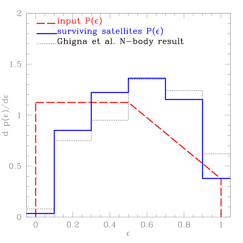
Figure 2: Input orbital circularity distribution of initially in-falling substructure (dashed) shown along with the circularity distribution of the final surviving population of ($n=1$) LCDM subhalos at $z=0$ (solid). For reference, the thin dotted line shows the circularity distribution of surviving substructure measured by Ghigna et al. (1998) in their N-body simulations.

To calculate the trajectories of subhalos, we treat them as point masses under the influence of the NFW gravitational potential of the host halo. We model orbital decay by dynamical friction using the Chandrasekhar formula (Chandrasekhar 1943). The Chandrasekhar formula was derived in the context of a highly idealized situation; however, numerical studies indicate that this approximate relation can be applied more generally (Valenzuela & Klypin 2003 have performed a new test that supports the use of this approximation). Using the Chandrasekhar approximation, there is a frictional force exerted on the subhalo that points opposite to the subhalo velocity:

$$F_{\rm DF}\simeq\frac{4\pi\ln(\Lambda)G^{2}M_{\rm sat}^{2}\rho(r)}{V_{\rm orb}^{2}}\Bigg{[}{\mathrm{erf}}(X)-\frac{2X}{\sqrt{\pi}}\exp(-X^{2})\Bigg{]}.$$ (4)

In equation (4), $\ln(\Lambda)$ is the Coulomb logarithm, $r$ is the radial position of the orbiting satellite, and $\rho(r)$ is the density of the host halo at the satellite radius. The quantity $V_{\rm orb}$ is the orbital speed of the satellite halo and $X\equiv V_{\rm orb}/\sqrt{2\sigma^{2}}$, where $\sigma$ is the one-dimensional velocity dispersion of particles in the host halo. For an NFW profile, the one-dimensional velocity dispersion can be determined using the Jeans equation. Assuming an isotropic velocity dispersion tensor,

$$\sigma^{2}(x=r/r_{s})=V_{\rm vir}^{2}\frac{c_{\rm vir}}{g(c_{\rm vir})}x(1+x)^{2}\int_{x}^{\infty}\frac{g(x^{\prime})}{x^{\prime 3}(1+x^{\prime})^{2}}{\mathrm{d}}x^{\prime}.$$ (5)

We find the following approximation useful and accurate to $1\%$ for $x=0.01-100$:

$$\sigma(x)\simeq V_{\rm max}\frac{1.4393x^{0.354}}{1+1.1756x^{0.725}}.$$ (6)

There has been much debate on the appropriate way to assign the Coulomb logarithm in Eq. (4). Dynamical friction is caused by the scattering of background particles into an overdense “wake” that trails the orbiting body and tugs back on the scatterer. The Coulomb logarithm is interpreted as $\ln(b_{\rm max}/b_{\rm min})$, where $b_{\rm max}$ is the maximum relevant impact parameter at which background particles are scattered into the wake and $b_{\rm min}$ is the minimum relevant impact parameter. A common approximation is to choose a constant value of the Coulomb logarithm (perhaps by calibrating to the results of numerical experiments as in TB01), but some studies indicate that this approach significantly underestimates the dynamical friction timescale when tested against N-body simulations (e.g., Colpi, Mayer, & Governato 1999; HFM02). Motivated by the results of HFM02 and Valenzuela & Klypin (in preparation), we allow the Coulomb logarithm to evolve with time and set $b_{\rm max}=r(t)$, where $r(t)$ is the radial position of the orbiting subhalo. We assign the minimum impact parameter according to the prescription of White (1976) and integrate the effect of encounters with background particles over the density profile of the subhalo. Repeating this calculation for an NFW halo yields

$$\ln(\Lambda)=\ln\Bigg{(}\frac{r}{R_{\rm sat}}\Bigg{)}+\frac{1}{g^{2}(x_{\rm sat})}I(x_{\rm sat}),$$ (7)

where

$$I(x_{\rm sat})\equiv\int_{0}^{x_{\rm sat}}x_{\rm b}^{3}\Bigg{[}\int_{x_{\rm b}}^{\infty}\frac{g(x)}{x^{2}\sqrt{x^{2}-x_{\rm b}^{2}}}\textrm{d}x\Bigg{]}^{2}\textrm{d}x_{\rm b},$$ (8)

$x_{\rm sat}\equiv R_{\rm sat}/r_{\rm s}^{\rm sat}$, and $r_{\rm s}^{\rm sat}$ is the NFW scale radius of the satellite. The integral $I(y)$ is well-approximated by the following function, which is accurate to $1\%$ for $0.1\leq y\leq 100$:

$$I(y)\simeq\frac{0.10947y^{3.989}}{[1+0.90055y^{1.099}+0.03568y^{1.189}+0.06403y^{1.989}]}.$$ (9)

As the satellite orbits within the host potential, it is stripped of mass by the tidal forces that it experiences. First, we estimate the instantaneous tidal radius of the subhalo $r_{\rm t}$, at each point along its orbit. In the limit that the satellite is much smaller than the host, the tidal radius is given by the solution to the equation (von Hoerner 1957; King 1962)

$$r_{\rm t}^{3}\simeq\frac{M_{\rm sat}(<r_{\rm t})/M_{\rm host}(<r)}{2+\omega^{2}R^{3}/GM_{\rm host}(<r)-\partial\ln M_{\rm host}(<r)/\partial\ln r}r^{3},$$ (10)

where $r$ is the radial position of the satellite, $M_{\rm host}(<r)$ is the host’s mass contained within this radius [cf. Eq. (3)], $M_{\rm sat}(<r_{\rm t})$ is the satellite’s mass contained within $r_{\rm t}$, and $\omega$ is the instantaneous angular speed of the satellite. Equation (10) is merely an estimate of the satellite’s tidal limit. For a satellite on a circular orbit, it represents the distance from the satellite center to the point along the line connecting the satellite and the host halo center where the tidal force on a test particle just balances the attractive force of the satellite. In reality, the tidal limit of a satellite cannot be represented by a spherical surface: some particles within $r_{\rm t}$ will be unbound while others without $r_{\rm t}$ may be bound. Nevertheless, TB01 showed that this can serve as a very useful approximation.

As the tidal radius shrinks, unbound mass in the periphery is stripped. Tidal forces are strongest, and $r_{\rm t}$ smallest, when the orbit reaches pericenter; however, all of the mass outside of $r_{\rm t}$ is not stripped instantaneously at each pericenter passage. Rather, mass is gradually lost from the satellite on a timescale set by the orbital energy of the liberated particles. Johnston (1998), found that the typical energy scale of tidally stripped debris is set by the change in the host halo potential on the length scale of the orbiting satellite, $\epsilon\approx r_{\rm t}\textrm{d}\Phi_{\rm host}(r)/\textrm{d}r$. Particles on circular orbits of energy $E$ and $E\pm\epsilon$ move a distance $r_{\rm t}$ relative to each other on a timescale of order the orbital period, $T$. As such, we may expect $T$ to be the relevant timescale for tidal mass stripping. TB01 used this timescale in their model to reproduce the results of several idealized N-body experiments. Following TB01, we model satellite mass loss by dividing the orbit into discrete time steps of size $\delta t\ll T$. At each step, we remove an amount of mass

$$\delta m=M_{\rm sat}(>r_{\rm t})\frac{\delta t}{T},$$ (11)

where $M_{\rm sat}(>r_{\rm t})$ is the satellite’s mass exterior to $r_{\rm t}$.

As a subhalo loses mass due to tidal stripping, we assume that its density profile is unmodified within its outer radius $R_{\rm sat}$. Rather than identify $R_{\rm sat}$ with the tidal radius (which does not vary monotonically with time), we set its value by determining the radius within which the mass profile retains the appropriate bound mass using Eq. (3). We fix the scale radius of the subhalo $r_{\rm s}^{\rm sat}$, at the value defined at the epoch of accretion.

Our approximations for dynamical friction and tidal stripping are least accurate when the mass of the satellite is not very small compared to the mass of the host. However, as $F_{\rm DF}\propto M_{\rm sat}^{2}$, it is in precisely these cases that we expect the satellite to merge quickly with the host and no longer be identifiable as distinct substructure. As such, the precise dynamics should not have a significant effect upon our results in these cases, particularly because our main predictions involve low-mass substructure. However, more detailed modeling will be important for investigations that focus on more massive substructures, for example, explorations that use disk thickening as a test of the $\Lambda$CDM cosmological model (e.g., Font et al. 2001).

The final ingredients for our semi-analytic model of halo substructure are the criteria for declaring subhalos to be tidally disrupted and centrally merged. Let $r_{\rm max}^{\rm sat}\simeq 2.16r_{\rm s}^{\rm sat}$ be the radius at which the subhalo’s initial velocity profile attains its maximum, and $M_{\rm sat}(<r_{\rm max}^{\rm sat})$ be the mass of the satellite originally contained within the radius $r_{\rm max}^{\rm sat}$. We declare a subhalo to be centrally merged with the host if its radial position relative to the center of the host becomes smaller than $r_{\rm max}^{\rm sat}$. We declare a satellite tidally disrupted if the mass of the satellite becomes less than $M_{\rm sat}(<r_{\rm max}^{\rm sat})$. This criterion is partially motivated by the numerical study of H03, who find that NFW subhalos are completely tidally destroyed shortly after $r_{\rm t}$ becomes less than $r_{\rm max}^{\rm sat}$. Of course the distinction between centrally merged and tidally destroyed satellites is somewhat arbitrary as subhalos are typically severely tidally disrupted as they approach the center of the host potential. Fortunately, for the issues we explore here, the precise nature of a satellite halo’s destruction is not important. We discuss this issue further in a forthcoming extension of our work (A. Zentner & J. Bullock, in preparation).

In reporting results concerning the velocity function of substructure, we invoke a further modification. H03 noted that subhalos that experienced significant tidal stripping suffered not only mass loss at radii $\lower 2.58334pt\vbox{\hbox{$\buildrel\textstyle>\over{\sim}\ $}}r_{\rm t}$, but mass redistribution in their central regions, at radii smaller than $r_{\rm t}$. To account for this, we determine whether or not the tidal radius of each surviving subhalo was ever less than $r_{\rm max}^{\rm sat}$. If so, we follow the prescription of H03 to account for mass redistribution and scale the maximum circular velocity of the satellite via

$$V_{\rm max}^{\rm final}=\Bigg{(}\frac{M_{\rm sat}^{\rm final}}{M_{\rm sat}^{\rm initial}}\Bigg{)}^{1/3}V_{\rm max}^{\rm initial},$$ (12)

where $V_{\rm max}^{\rm initial}$ is the maximum circular velocity of the satellite according to its initial density profile, $M_{\rm sat}^{\rm final}$ is its final mass, and $M_{\rm sat}^{\rm initial}$ is its initial mass before being tidally stripped. In practice, this rescaling has a fairly small effect on our velocity functions. Roughly $\sim 30\%$ of surviving halos meet this condition for $r_{\rm t}$. For those halos that do experience this kind of mass loss, the typical reduction in $V_{\rm max}$ is $\lower 2.58334pt\vbox{\hbox{$\buildrel\textstyle<\over{\sim}\ $}}25\%$.

We are currently in the process of checking this model against idealized N-body experiments designed to mimic the type of orbital histories that we encounter here (J. Bullock, K. Johnston, & A. Zentner, in preparation). Preliminary results show promising agreement.

Orbital evolution for three sets of subhalo parameters: $M_{sat}^{0}=10^{8}$ M_⊙ , $c_{\rm vir}=15$ (solid); $M_{sat}^{0}=10^{8}$ M_⊙ , $c_{\rm vir}=7.5$ (dashed); and $M_{sat}^{0}=5\times 10^{9}$ M_⊙ , $c_{\rm vir}=15$ (short-dashed). Initial orbital parameters and host mass properties are fixed, as described in the text. The top panel shows the radial evolution in units of the initial radius as a function of time. The bottom panel shows the mass of each system as a function of time. Lines that terminate represent subhalo destruction at the end point (see text).

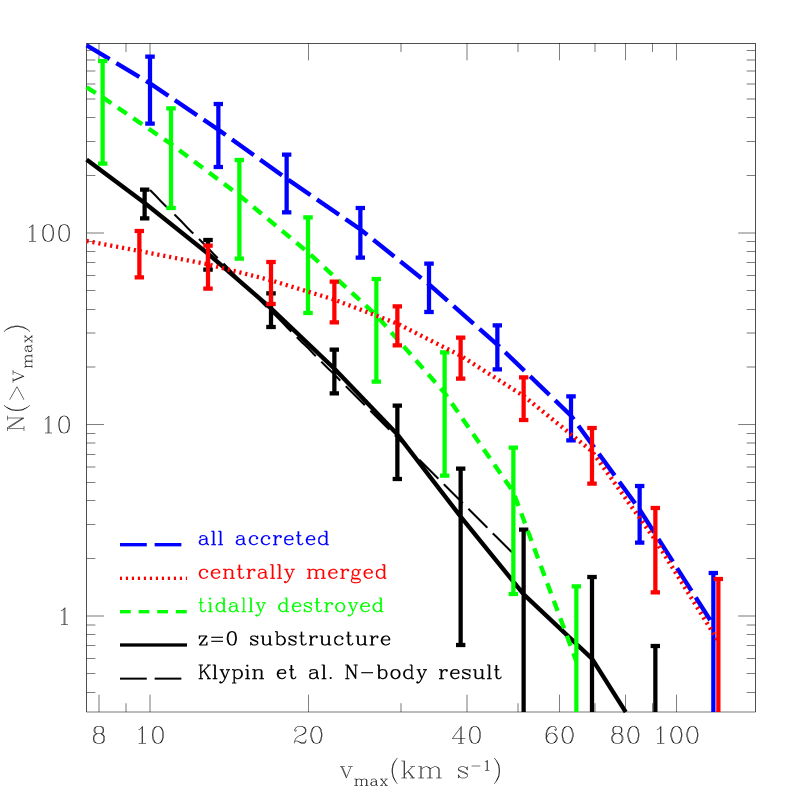
Figure 3: The velocity functions of progenitor and surviving subhalo populations derived using our fiducial ($n=1$, $\sigma_{8}=0.95$) $\Lambda$CDM cosmology and a 200-halo ensemble of $1.4\times 10^{12}$ M_⊙ systems at $z=0$. Shown are all accreted halos (dashed), and the fraction of those that are tidally destroyed (short-dashed) and centrally merged (dotted). The solid line shows the surviving population of subhalos at $z=0$ and, for comparison, the thin dashed line shows the surviving population derived by K99 using N-body simulations. The error bars represent the sample variance.

2.4 Tests and Examples

Figure 2.3 shows three example calculations of subhalo trajectories aimed at demonstrating how various factors affect the orbital evolution of a satellite system. Each satellite was started on the same initial orbit, $\epsilon=\eta=0.5$, but the satellite properties were varied: $M_{\rm sat}^{0}=10^{8}$ M_⊙, $c_{\rm vir}=15$ (solid); $M_{\rm sat}^{0}=10^{8}$ M_⊙, $c_{\rm vir}=7.5$ (dashed); and $M_{\rm sat}^{0}=5\times 10^{9}$ M_⊙, $c_{\rm vir}=15$ (short-dashed). The upper and lower panels depict the evolution of orbital radius and mass of the subhalo respectively. The accretion time was set at $8$ Gyr in the past, $a=(1+z)^{-1}\simeq 0.45$ for this cosmology. The host halo parameters were chosen to match reasonable expectations for a Milky Way-sized progenitor at that time: $M_{\rm host}=5\times 10^{11}$ M_⊙ ($R_{\rm vir}\simeq 110$kpc) and $c_{\rm vir}=6$. While the subhalo represented by the solid line experiences gradual tidal mass loss and slight orbital decay as a result of dynamical friction, its core survives for the full time period. The less concentrated subhalo (dashed) is more strongly affected by tides, and is completely disrupted $\sim 3.5$ Gyr after being incorporated into the host. (Although not shown, a similar effect is seen if the host halo concentration is increased and the subhalo concentration is held fixed.) In the case of the massive subhalo, dynamical friction causes the orbit to decay more quickly and the subhalo experiences more frequent pericenter passages. Consequently, disruption occurs $\sim 6$ Gyr after accretion. Notice that because the stripping process is gradual (unless orbits are very radial) and the timescales involved are of order $\sim$ Gyr, the accretion time is also important in determining survival probability. If any of these subhalos were were accreted more recently, their chance of survival to the present day would increase accordingly. The combination of factors illustrated here — accretion time, satellite mass, and the relative concentrations of host and satellite — will be important in later sections for understanding the factors that set the subhalo population from one cosmology to the next.

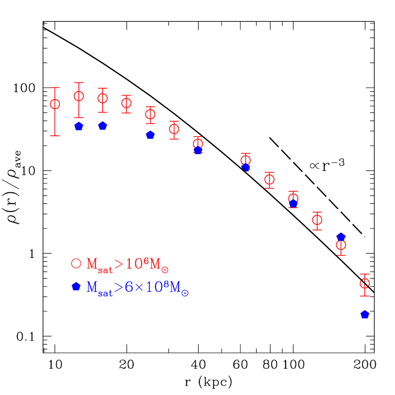
Figure 4: The radial number density profile of substructure derived from 200 model realizations of a $M_{\rm vir}=1.4\times 10^{12}$ M_⊙ host halo at $z=0$ in our fiducial ($n=1$, $\sigma_{8}=0.95$) $\Lambda$CDM cosmology. The open circles show the number density of subhalos with $M_{\rm sat}>10^{6}$ M_⊙ divided by the average number density of systems meeting this mass threshold within the virial radius of the host system. The points reflect the radial profile averaged over all realizations, and the error bars reflect the sample variance. Solid pentagons show the same result for $M_{\rm sat}>6\times 10^{8}$ M_⊙ subhalos. The variance (not shown) is significantly larger for the higher mass threshold because there are significantly fewer such systems in each host. For reference, the solid line shows the NFW density profile of the host at $z=0$. The virial radius for a host halo of this size is $R_{\rm vir}\simeq 285$ kpc and the typical NFW scale radius is $r_{\rm s}\simeq 20$ kpc. We do not plot predictions beyond $r=0.75R_{\rm vir}\simeq 215$ kpc because this is the maximum circular radius we assign to in-falling, bound systems.

Figure 3 shows the ensemble-averaged, cumulative velocity function for the substructure population of Milky Way-like host halos computed in our standard $\Lambda$CDM cosmology. The host properties at $z=0$ are $M_{\rm vir}=1.4\times 10^{12}$ M_⊙, $c_{\rm vir}\simeq 13.9$, and $V_{\rm max}\simeq 187\textrm{ km s}^{-1}$. The lines represent the means of 200 merger tree realizations, and the error bars represent the sample variances over these realizations. In particular, the thick solid line shows the surviving subhalo population at $z=0$. For comparison, the thin dashed line is the best-fit velocity function reported by K99 based on an analysis of substructure in $\Lambda$CDM halos. This line is plotted over the range that their resolution and sample size allowed them to probe. The apparent agreement between our semi-analytic model and the N-body result is excellent, and lends confidence in our ability to apply this model to different power spectra.

The radial distribution of substructure at $z=0$ for the same ensemble of halos is shown in Figure 4. Open circles show the differential number density profile of subhalos with $M_{\rm sat}>10^{6}$ M_⊙ normalized relative to the total, volume-averaged number density of subhalos within $R_{\rm vir}$ that meet the same mass requirement. The solid pentagons show the same quantity for more massive subhalos, $M_{\rm sat}>6\times 10^{8}$ M_⊙. The line shows the NFW dark matter profile for the host system normalized relative to the average (virial) density within the halo. Observe that the subhalo profile traces the dark matter profile at large radius ($\rho\propto r^{-3}$), but flattens towards the center as a consequence of tidal disruption. This result agrees well with that presented in Figure 3 of Colín et al. (1999). Using an N-body analysis of a cluster-sized host, Colín et al. (1999) showed that the number density of systems with $M_{\rm sat}$ greater than $0.04\%$ of the host mass traces the background halo profile at large radius, begins to flatten at $r\sim 0.2R_{\rm vir}$, and is roughly a factor of $5$ below the background at $r\sim 0.07R_{\rm vir}$ (their innermost point). The solid pentagons in Figure 4 correspond to the same mass fraction relative to the host. Notice that at $r=0.07R_{\rm vir}\simeq 20$ kpc, the factor of $\sim 5$ mismatch is reproduced. Ghigna et al. (1998) observed the same qualitative behavior for subhalos in a standard CDM simulation of a cluster-size halo. Chen et al. (2003) have measured the substructure profile using a high-resolution galaxy-size halo with $M_{\rm sat}\lower 2.58334pt\vbox{\hbox{$\buildrel\textstyle>\over{\sim}\ $}}0.0015\%M_{\rm host}$, corresponding to subhalos intermediate in mass between those represented by the open circles and solid pentagons in Figure 4. Chen et al. (2003) similarly find core behavior setting in at a radius of $\sim 30$ kpc, but also find a stronger overall suppression in substructure counts within $r\lower 2.58334pt\vbox{\hbox{$\buildrel\textstyle<\over{\sim}\ $}}70$ kpc. Our results suggest that some of the observed suppression may be caused by overmerging in the central regions of their simulated halos. Ongoing studies by other workers lead to similar conclusions (J. Taylor, private communication). Only the next generation of numerical simulations can reliably test this. That we produce a reasonable approximation to the number density profile of substructure is an indication of the soundness of our model.

3 Model Power Spectra

The initial power spectrum of density fluctuations is conventionally written as an approximate power law in wavenumber $k$, $P(k)\propto k^{n}$, corresponding to a variance per logarithmic interval in wavenumber of $\Delta^{2}(k)=k^{3}P(k)/2\pi^{2}$. If the fluctuations were seeded during an early inflationary stage, as is commonly supposed, then the initial spectrum is likely to be nearly scale-invariant, with $n\simeq 1$. Any deviation from power law behavior, or “running” of the power law index with scale is likewise expected to be small, $|\textrm{d}n/\textrm{d}\ln k|<0.01$ (Kosowsky & Turner 1995). In addition to these theoretical prejudices, large-scale observations of galaxy clustering and CMB anisotropy seem to favor nearly scale-invariant models that can be parameterized in this way. In this paper we explore the effects on halo substructure of taking $n\neq 1$ and allowing for scale-dependence in the power law index and more dramatic features in the power spectrum. In this section we give a brief description of the power spectra that we explore.

Table 1 summarizes the relevant features of our example power spectra. The second and third columns list the primordial spectral index evaluated at the pivot scale of the COBE measurements $k_{\rm COBE}\approx 0.0023$ h Mpc^-1, and the running of the spectral index. We neglect any variation in the running with scale and explicitly set $\textrm{d}^{2}n(k)/\textrm{d}(\ln k)^{2}=0$. Except for the running index (RI) case, we normalize all models to the COBE measurements of the CMB anisotropy using the fitting formulae of Bunn, Liddle, & White (1996; also Bunn & White 1997). The fourth column of Table 1 gives the implied value of $\sigma_{8}$. We calculate spectra using the transfer functions of Eisenstein & Hu (1999). In Figure 5 we illustrate the implied $\sigma(M)$ for these models.

Many of the spectra listed in Table 1 are motivated by particular models of inflation. We invoke an inverse power law potential that gives rise to a mild tilt $n\simeq 0.94$, as well as a model in which the inflaton has a logarithmically running mass and which can give rise to significant tilt and running for natural parameter choices (Stewart 1997a,b; Covi & Lyth 1999; Covi, Lyth, & Roszkowski 1999; Covi, Lyth, & Melchiorri 2003). We employ specific inflationary potentials mainly as a conceptual follow up to ZB02, which highlighted the fact that various levels of tilt may occur naturally within the paradigm of inflation and that $n\equiv 1$ is not demanded by this paradigm. For the purposes of this paper, one may regard our choices simply as spanning a range of observationally viable input power spectra. The values of tilt and $\sigma_{8}$ that we consider range from $n\simeq 0.84$ with $\sigma_{8}=0.65$ to $n=1$ and $\sigma_{8}=0.95$. The model with $\sigma_{8}=0.75$ was specifically chosen to match galaxy central densities, as described in ZB02. We also explore the best-fit, running-index model of the WMAP team (Spergel et al. 2003), with ${\rm d}n/{\rm d}\ln k=-0.03$. We refer to this as the “running index model” or “RI model.” Note that Spergel et al. (2003) quote a value of $n=0.93$ evaluated at $k=0.05$ Mpc^-1. The value listed in Table 1 is larger because we quote it at a smaller wavenumber, $k=k_{\rm COBE}$.

In addition to tilted $\Lambda$CDM models, we consider spectra with abrupt reductions in power on small scales. In the “broken scale-invariance” (BSI) example, we adopt an idealized inflation model introduced by Starobinsky (1992) that exhibits the most rapid drop in power possible for a single field model. Kamionkowski & Liddle (2000) studied this type of model as a way to mitigate the dwarf satellite problem, but our choice of parameters is slightly different from theirs (see ZB02).

We also consider WDM scenarios in which the primordial power spectra are scale-invariant but small-scale fluctuations are subsequently filtered by free-streaming. The free-streaming scale is set by the primordial velocity dispersion of the warm particles. In the canonical case of a “neutrino-like,” thermal relic with two internal degrees of freedom, the free-streaming scale can be expressed in terms of the warm particle mass $m_{\rm W}$ and relic abundance, $\Omega_{\rm W}h^{2}$:

$$R_{f}\simeq 0.11\left[\frac{\Omega_{\rm W}h^{2}}{0.15}\right]^{1/3}\left[\frac{m_{\rm W}}{{\rm keV}}\right]^{-4/3}{\rm Mpc}.$$ (13)

We calculate WDM spectra assuming the same flat cosmology with $\Omega_{\rm M}=\Omega_{\rm W}+\Omega_{\rm B}=0.3$, and use the approximate WDM transfer function given by Bardeen et al. (1986), $P(k)=\exp[-kR_{f}-(kR_{f})^{2}]P_{\rm CDM}(k)$.

Several studies have placed approximate constraints on WDM masses based on either the argument that there must be enough power on small scales to reionize the Universe at sufficiently high redshift ($z_{\rm re}\lower 2.58334pt\vbox{\hbox{$\buildrel\textstyle>\over{\sim}\ $}}6$) or by probing the power spectrum on small scales directly with the Ly-$\alpha$ forest (Barkana, Haiman, & Ostriker 2001; Narayan et al. 2000). These authors essentially find that $m_{\rm{\rm W}}\lower 2.58334pt\vbox{\hbox{$\buildrel\textstyle>\over{\sim}\ $}}0.75$ keV assuming a neutrino-like thermal relic; however, this constraint may be significantly more restrictive if measurements of $z_{\rm re}\sim 17$ by the WMAP collaboration (Kogut et al. 2003; Spergel et al. 2003) are confirmed (Somerville, Bullock, & Livio 2003). As such, we consider three illustrative examples in what follows, $m_{\rm W}=0.75$ keV, $1.5$ keV, and $3.0$ keV. The corresponding “free-streaming” masses, below which the fluctuation amplitudes are suppressed, are listed in Table 1.

4 RESULTS

4.1 Accretion Histories

Our first results concern the merger histories of halos that are approximately Milky Way-sized, with $M_{\rm vir}=1.4\times 10^{12}$ M_⊙ at $z=0$. For the $n=1$, $\Lambda$CDM model, we present results based on 200 realizations. For all other models, our findings are based on 50 model realizations.

Table 1: Summary of power spectra properties

Model Description	$n(k_{\rm COBE})$	$\textrm{d}n(k)/\textrm{d}\ln k$	$\sigma_{8}$	comments
Scale-invariant	$1.00$	$0.000$	$0.95$
Inverted power law inflation	$0.94$	$-0.002$	$0.83$
Running-mass inflation I	$0.84$	$-0.008$	$0.65$	see Stewart 1997a,b
Running-mass inflation II	$0.90$	$-0.002$	$0.75$
WMAP best-fit running index (RI) model	$1.03$	$-0.03$	$0.84$	WMAP best fit, see Spergel et al. 2003
Broken scale-invariant inflation (BSI)	$1.00$	$0.000$	$0.97$	exhibits sharp decline in power at $k\lower 2.58334pt\vbox{\hbox{$\buildrel\textstyle>\over{\sim}\ $}}1$ h Mpc-1,
				power suppressed for $M\lower 2.58334pt\vbox{\hbox{$\buildrel\textstyle<\over{\sim}\ $}}10^{10}$ M⊙
Warm Dark Matter, $m_{\rm W}=3.0$ keV	$1.00$	$0.000$	$0.95$	$M_{f}\simeq 8.3\times 10^{8}$ M⊙
Warm Dark Matter, $m_{\rm W}=1.5$ keV	$1.00$	$0.000$	$0.95$	$M_{f}\simeq 1.3\times 10^{10}$ M⊙
Warm Dark Matter, $m_{\rm W}=0.75$ keV	$1.00$	$0.000$	$0.94$	$M_{f}\simeq 2.1\times 10^{11}$ M⊙

Note. — Column (1) gives a brief description of the inflation or warm dark matter model used to predict the power spectrum. In the text, we distinguish the first five models by their tilts and/or their values of $\sigma_{8}$. We label the warm dark matter models by the warm particle mass. Columns (2) and (3) give the tilt $n(k_{\rm COBE})$ on the pivot scale of the COBE data $k_{\rm COBE}\approx 0.0023$ h Mpc^-1, and the running of the spectral index $\textrm{d}n(k)/\textrm{d}\ln k$, respectively. We have explicitly assumed the “running-of-running” to be small and taken $\textrm{d}^{2}n(k)/\textrm{d}(\ln k)^{2}=0$. Column (4) contains the values of $\sigma_{8}$ implied by the tilt or warm particle mass, the COBE normalization, and our fiducial cosmological parameters except in the case of the WMAP best-fit running index (RI) model, in which case the value of $\sigma_{8}$ reflects their best-fit normalization.

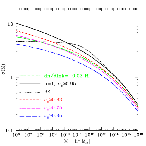
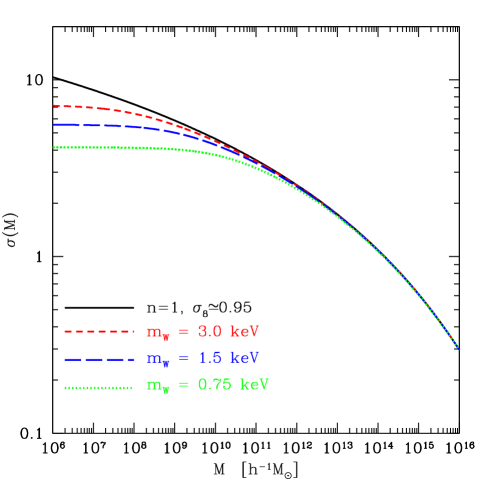
Figure 5: The $z=0$ rms overdensity as a function of mass scale for several of our adopted power spectra (see §3 and Table 1 for more details). In the left panel, we exhibit spectra that deviate from the standard $n=1$, scale-invariant model. The models shown in this panel are standard $n=1$ (solid), a broken scale-invariant model (dotted), $\sigma_{8}=0.84$ & $n\simeq 0.94$ (short-dashed), $\sigma_{8}=0.65$ & $n\simeq 0.84$ (long-dashed), $\sigma_{8}=0.75$ & $n\simeq 0.90$ (dot-long-dashed), and a model based on the results of the WMAP team with $n\simeq 1.03$, $\textrm{d}n/\textrm{d}\ln k=-0.03$, and $\sigma_{8}=0.84$ (dot-short-dashed). The inflation models that inspire these examples are described in ZB02. In the right panel, we show several warm dark matter power spectra. More precisely, we depict spectra implied by warm particle masses of $m_{\rm W}=3.0$ keV (short-dashed), $m_{\rm W}=1.5$ keV (long-dashed), and $m_{\rm W}=0.75$ keV (dotted) along side the standard $n=1$, $\Lambda$CDM spectrum (solid).

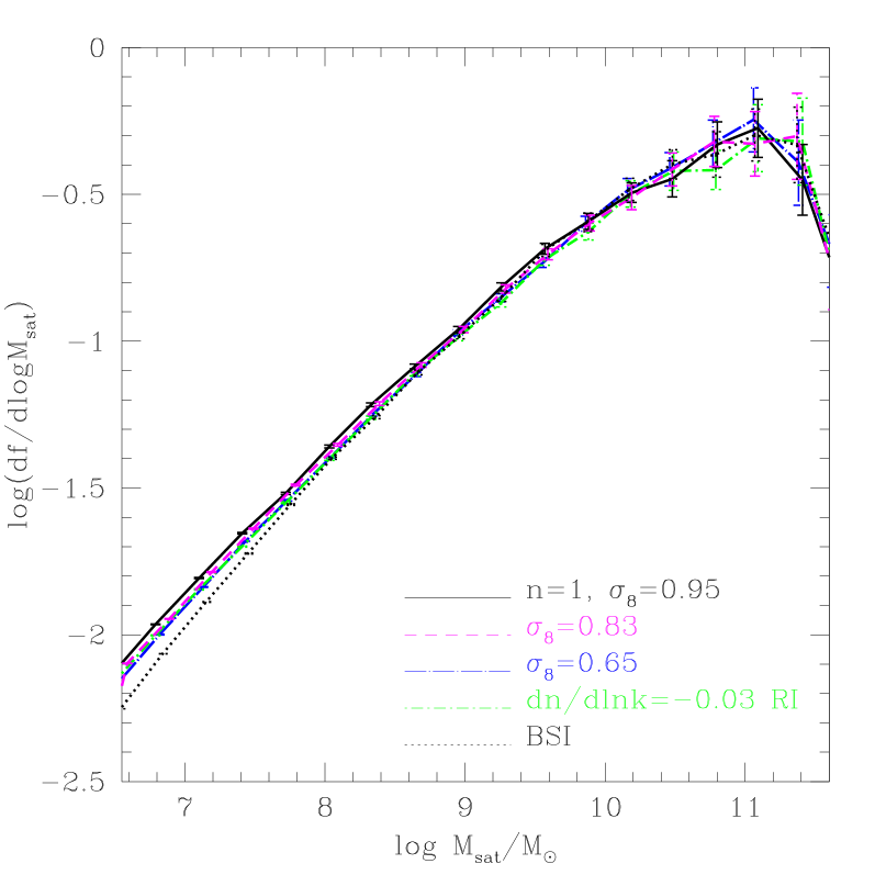
Figure 6: Fraction of final host mass accreted in subhalos of mass $M_{\rm sat}$ as a function of $M_{\rm sat}$. The final host mass is $1.4\times 10^{12}$ M_⊙. The results for several input power spectra are shown.

Figure 6 focuses on the the mass distribution of accreted halos, integrated over the entire merger history of the host. We plot $\textrm{d}f/\textrm{d}\log(M_{\rm sat})$, the fraction of mass in the final halo that was accreted in subhalos of a given mass per logarithmic interval in subhalo mass, $M_{\rm sat}$. Observe that the mass fraction accreted in subhalos of a given mass is relatively insensitive to the shape of the power spectrum. Although similarity from model to model may be somewhat surprising at first, it follows directly from repeated application of Equation (1). In particular, the shape of the progenitor distribution for $M_{\rm sat}\ll M_{\rm host}$ must follow $\textrm{d}f/\textrm{d}\log(M_{\rm sat})\propto M_{\rm sat}^{1/2}$, and the turnover occurs because mass conservation suppresses the number of major mergers. The shape shown in Figure 6 and its insensitivity to the power spectrum is discussed in detail by LC93.

While the total mass function of accreted substructure is relatively independent of the power spectrum, the merger histories themselves are not. In models with less power on galaxy scales, halos assemble their mass later and experience more recent mergers and disruption events. We show an example of this in Figure 7. Here we plot the average accretion rate of subhalos with $M_{\rm sat}>10^{8}$ M_⊙ for host halos in the standard $n=1$, $\Lambda$CDM model, the RI model, and our lowest normalization case ($n=0.84$, $\sigma_{8}=0.65$). The total accretion rate is divided in two pieces: dashed lines show those subhalos that are eventually destroyed and solid lines show the accretion times of subhalos that survive until $z=0$. For the standard ($n=1$, $\sigma_{8}=0.95$) case, the event rate peaks sharply about $\sim 12$ Gyr in the past, while the $\sigma_{8}=0.65$ case has a broader distribution, peaking later at $\sim 9$ Gyr ago, and with a long tail of accretion events extending towards the present day.

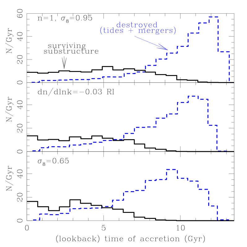
Figure 7: Accretion rate averages, $dN/dt$ (Gyr^-1), for merged halos more massive than $10^{8}$ M_⊙ and host halos of mass $1.4\times 10^{12}$ M_⊙ at $z=0$. Three different power spectra are shown: $n=1$ (upper); RI model (middle); and $n=0.84$, $\sigma_{8}=0.65$ (bottom). Dashed lines show objects that are destined to be destroyed, either by tidal disruption or central merging, and solid lines show subhalos that survive until $z=0$. The $n=1$ results are based on 200 EPS realizations while the others are based on 50 realizations.

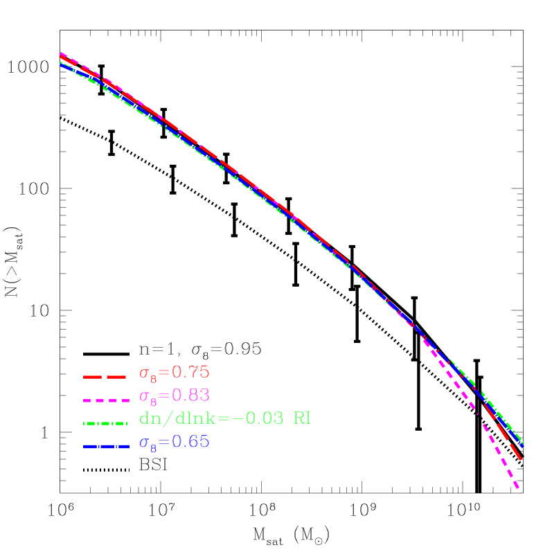
Figure 8: The cumulative mass function $N(>M)$, of surviving subhalos computed for an ensemble of host halos of mass $M_{\rm host}=1.4\times 10^{12}M_{\odot}$ at $z=0$. The lines show the means computed over all realizations. The different line types relate to different models following the convention in the left panel of Figure 5. The $n=1$ results are derived from 200 realizations and the results for the other models are based on 50 realizations. The error bars show the variance over the $n=1$ realizations (upper) and BSI realizations (lower).

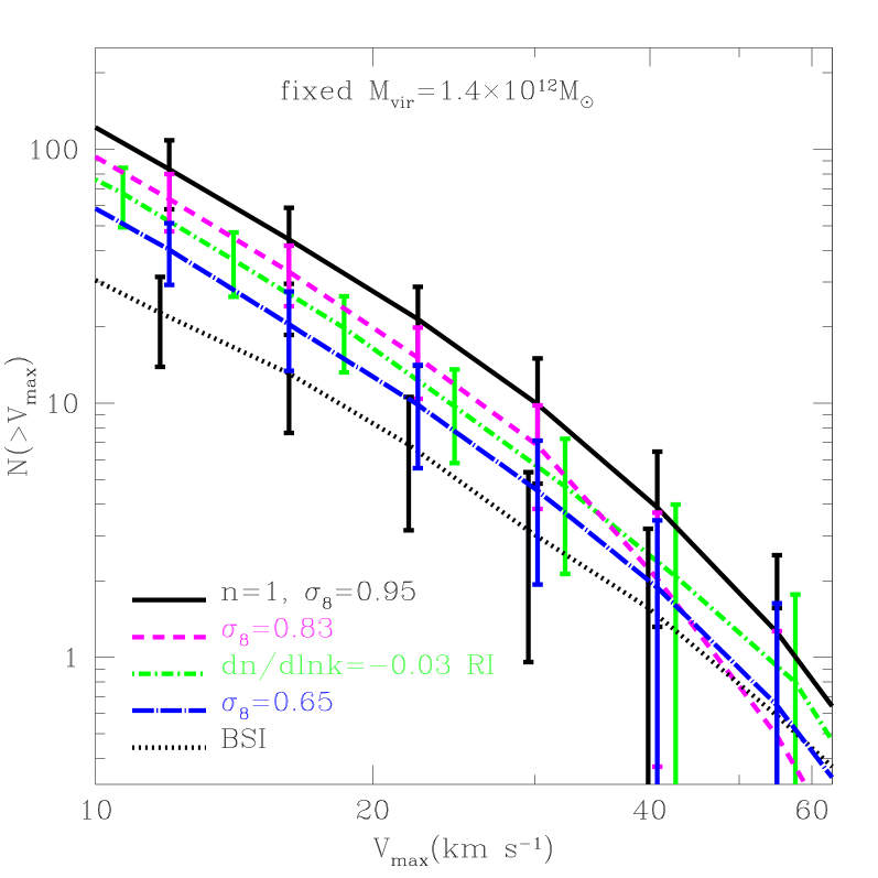
Figure 9: The cumulative velocity function of subhalos in a host of fixed mass, $M_{\rm host}=1.4\times 10^{12}$ M_⊙. The lines represent averages over 200 merger histories for $n=1$ and 50 merger histories for the other models. The error bars represent the dispersion amongst these realizations. The models are $n=1$ (solid), $\sigma_{8}\simeq 0.83$ (dashed), RI model (dot-short-dashed), $\sigma_{8}\simeq 0.65$ (dot-long-dashed), and BSI (dotted).

The shift in accretion times in models with less small-scale power plays an important role in regulating the number of surviving subhalos. As we discussed in relation to Figure 2.3, a finite amount of time is required for an orbit to decay or for a system to become unbound and in many cases the longer a subhalo orbits in the background potential, the more probable its disruption becomes. The later accretion times in models with less power partially compensate for the fact that subhalos in these models are less centrally concentrated and more susceptible to disruption at each pericenter passage. Particular results for substructure populations in each model are given in the following subsections.

That we expect a characteristic merger/disruption phase in each halo’s past is intriguing, as this phase is approximately coincident with the estimated ages of galactic thick disks, $t_{td}\sim 8-10$ Gyr (e.g., Quillen & Garnett 2000 for the Milky Way), which seem to be ubiquitous and roughly coeval (Dalcanton & Bernstein 2002). In this context, the age distributions of thick disks might serve as a test of this characteristic accretion time, which varies as a function of normalization and cosmology. We reiterate that the look-back times shown for the dashed lines in Figure 7 are the times that the subhalos were accreted. The distributions of central merger rates and tidal destruction rates peak at slightly more recent times and their widths are broader, with longer tails towards the present epoch.

It is interesting to note that the surviving halos in Figure 7 represent a distinctly different population of objects than the destroyed systems — they tend to have been accreted more recently. We are inclined to speculate that the star formation histories of galaxies that were destroyed after being accreted could be distinctly different from those of the surviving (dwarf satellite) galaxies as well. This may have implications for understanding whether the stellar halo of our Galaxy formed from disrupted dwarfs or some other process. While the global structure of the stellar halo seems consistent with the disruption theory (Bullock, Kravtsov, & Weinberg 2001), the element ratios of stellar halo stars and stars in dwarf galaxies are not consistent with a common history of chemical evolution (Shetrone, Côte, & Sargent 2001). The results shown in Figure 7 provide general motivation to model dwarf galaxy evolution and Milky Way formation in a cosmological context.

4.2 Mass and Velocity Functions

We present our results on CDM halo substructure beginning with the abundance of satellites in Milky Way-like galaxies. We plot the mass function of subhalos $N(>M_{\rm sat})$, or the number of subhalos with mass greater than $M_{\rm sat}$ as a function of $M_{\rm sat}$, for each of our models in Figure 8. The host halo mass is again fixed at $1.4\times 10^{12}$ M_⊙ at $z=0$. From this figure, we see that even in the significantly tilted, low-normalization model ($\sigma_{8}\simeq 0.65$), the number of satellite halos with mass greater than $10^{6}$ M_⊙ is roughly equal to that in the standard $n=1$ model. The systematic differences between models are small compared to the scatter. The suppression is weak because several competing effects tend to compensate for the reduced concentrations of the subhalos. In tilted models with reduced small-scale power, subhalos are typically accreted at later times. In addition, host halos are less concentrated and correspondlingly less capable of disrupting their satellites.

In contrast, the BSI model shows a substantial decrease (a factor of $\sim 3$) in the number of surviving satellite halos at fixed mass. The reason for the dramatic reduction in this case is easy to understand. First, power is reduced only on scales smaller than a critical scale around $\sim 10^{10}$ M_⊙ (cf. Figure 5) and so, the concentration and accretion history of the $\sim 10^{12}$ M_⊙ host halo are minimally altered while the concentrations of the small subhalos are drastically reduced (see ZB02). In other words, the host halo has a density structure similar the $n=1$ model host and is just as capable of tidally disrupting satellites, but the satellites are significantly more susceptible to disruption. A second difference is that galaxy-size halos in the BSI model, unlike the tilted models, accrete $\sim 40\%$ fewer low-mass ($\lower 2.58334pt\vbox{\hbox{$\buildrel\textstyle<\over{\sim}\ $}}10^{7}$ M_⊙ ) halos over their lifetimes, and this further widens the disparity between the BSI and tilted-$\Lambda$CDM models.

It is conventional to discuss the substructure population of Milky Way-like halos in terms of the velocity function. In Figure 9, we show our results for the cumulative velocity functions of subhalos for a fixed host mass of $M_{\rm host}=1.4\times 10^{12}$ M_⊙. Notice that the velocity functions show a stronger trend with power spectrum than the mass functions (Figure 8), but the effect is still modest compared to the statistical scatter. For the most extreme tilted model, the total number of subhalos with $V_{\rm max}\lower 2.58334pt\vbox{\hbox{$\buildrel\textstyle>\over{\sim}\ $}}10\textrm{ km s}^{-1}$ is only a factor of $\sim 2$ lower than in the standard, scale-invariant case. In the case of the tilted models, the reduction in the velocity function is largely due to the fact that the subhalos are less concentrated, so the $V_{\rm max}$ values are correspondingly smaller for fixed halo masses [cf. Eq. (3) and the discussion that follows].

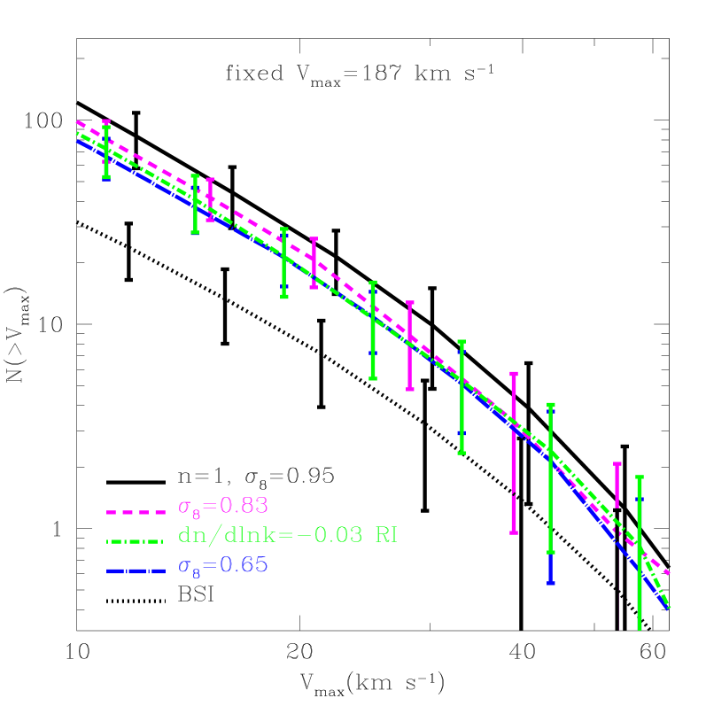
Figure 10: The cumulative velocity function of subhalos in a host of fixed maximum velocity $V_{\rm max}\simeq 187\textrm{ km s}^{-1}$. The lines represent averages over 200 merger history realizations for $n=1$ and 50 realizations for all other models. The error bars represent the dispersion in these realizations. The different models are as in Figure 9.

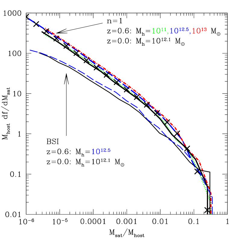
Figure 11: The average differential mass fraction, $df/dM_{\rm sat}$, normalized relative to host mass and satellite mass. The upper set of (bold) curves were computed for the $n=1$ cosmology with $M_{\rm host}=1.4\times 10^{12}$ M_⊙ at $z=0$ (solid) and $M_{\rm host}=$ $10^{11}$ M_⊙ (dotted), $3\times 10^{12}$ M_⊙ (long-dash) and $10^{13}$ M_⊙ (dot-dash) all at $z=0.6$. The lower set of thin curves correspond to BSI halos of $M_{\rm host}=1.4\times 10^{12}$ M_⊙ at $z=0$ (solid) and $M_{\rm host}=3\times 10^{12}$ M_⊙ at $z=0.6$ (long-dash). The crosses reflect an analytic fit to the $n=1$ results, as discussed in the text [see Eq. (14)].

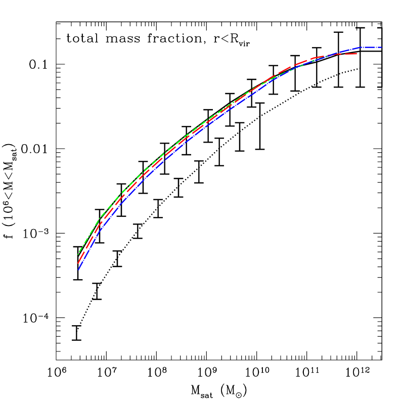
Figure 12: The fraction of the parent halo mass that is bound up in substructure in the mass range between $10^{6}$ M_⊙ and $M_{\rm sat}$ as a function of $M_{\rm sat}$. The host halo in each case has $M=3\times 10^{12}$ M_⊙ at $z=0.6$. Lines reflect the mean over all realizations, and results are shown for the $n=1$ model (solid), RI model (dot-short-dash), $\sigma_{8}=0.75$ (dashed), $\sigma_{8}=0.65$ (dot-long-dash), and BSI (dotted). The error bars on the top set of lines reflect the $90$ percentile range determined using $200$ merger tree realizations for the $n=1$ case (the other models in the top set of lines have very similar scatter). The bottom set of errors reflect the same range determined using $50$ realizations of the BSI model.

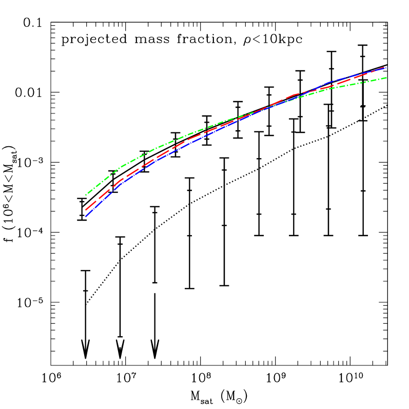
Figure 13: The fraction of mass in substructure in a central, cylindrical projection of radius $10$ kpc, for the same set of halos as shown in Figure 12. The line types are the same as those in Figure 12, and again represent the mean fraction computed over all realizations. The large and small error bars represent the $90$ and $64$ percentile ranges, respectively. A down-arrow is plotted instead of a lower, large error tick if at least $5\%$ of the realizations had $f=0$ in that bin. A down-arrow with no accompanying lower error bar means that at least $18\%$ of the realizations were without projected substructure in that bin.

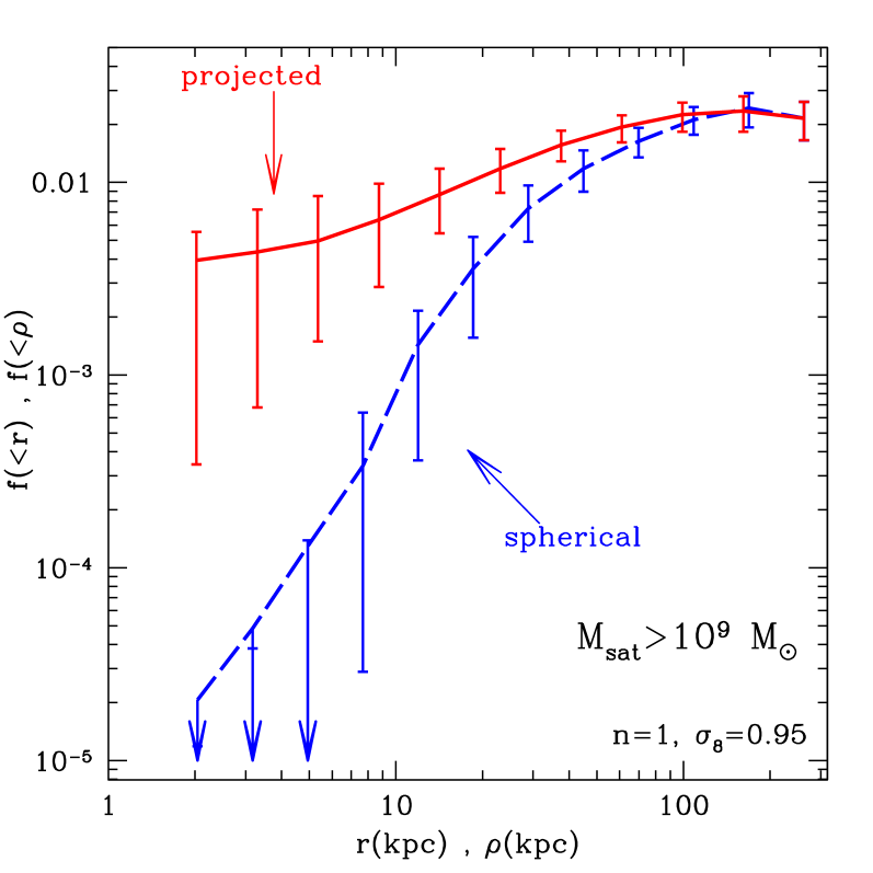
Figure 14: The cumulative mass fraction of substructure with $10^{6}$ M_⊙ $<M_{\rm sat}<10^{9}$ M_⊙ shown spherically averaged as a function of radius $r$ (solid line) and in projection, as a function of the projected radius $\rho$ (dashed line). The averages (lines) and $64\%$ percent ranges (error-bars) were determined using $200$ realizations of $M=3\times 10^{12}$ M_⊙ halos $z=0.6$ for our $n=1$ model. Down-arrows indicate that more than $18\%$ of the realizations had $f=0$ in the corresponding radial bin.

This effect is illustrated explicitly in Figure 10 where, rather than fixing the host mass at $z=0$, we have fixed its maximum circular velocity at $V_{\rm max}=187\textrm{ km s}^{-1}$, the value of a typical $n=1$, $M_{\rm host}=1.4\times 10^{12}$ M_⊙ halo at $z=0$. Normalizing our host halos by $V_{\rm max}$ rather than mass is perhaps a more reasonable choice because $V_{\rm max}$ is more closely related to observations. Models with less galactic-scale power require a more massive host in order to obtain the same value of $V_{\rm max}$, and their velocity functions shift correspondingly. For example, a host with $V_{\rm max}=187\textrm{ km s}^{-1}$ in the $\sigma_{8}=0.65$ model requires $M_{\rm host}\approx 2.2\times 10^{12}$ M_⊙. With this adjustment, the velocity functions of the various tilted models are now very similar. Again, the BSI case is different from the tilted models because the relative shift in the $V_{\rm max}$-$M_{\rm vir}$ relation changes abruptly with mass scale. It is also encouraging that our model BSI velocity function agrees well with the N-body results of Colín et al. (2000) for a similar type of truncated power spectrum (see their $R_{f}=0.1$ Mpc model, Fig. 2).

Another convenient way to quantify the substructure content of halos is the fraction of mass in subhalos less massive than $M_{\rm sat}$, $f(<M_{\rm sat})$. Figure 11 shows the differential mass fraction $df/dM_{\rm sat}$, normalized relative to the host mass for several different host masses and redshifts in both the $n=1$ and BSI models. The results are approximately self-similar with respect to the host mass, and for the $n=1$ case can be well-represented by the analytic form

$$\frac{{\rm d}f}{{\rm d}x}=\left[\frac{x}{x_{0}}\right]^{-\alpha}\exp\left[-\frac{x}{x_{0}}\right],$$ (14)

with $x\equiv M_{\rm sat}/M_{\rm host}$, $\alpha=0.6$ and $x_{0}=0.07\pm 0.05$. The quoted range in $x_{0}$ characterizes well the rms scatter from realization to realization (not shown). This function (with $x_{0}=0.07$) is shown as the set of crosses in Figure 11. As expected, the mass fractions are somewhat lower for the BSI model halos. The other CDM-type models all yield differential mass functions similar to those of the $n=1$ case. While in the next section we present results for a particular choice of host mass, the self-similarity demonstrated here implies that results at a fixed satellite-to-host mass ratio $x$, can be scaled in order to apply these results to any value of $M_{\rm host}$.

4.3 Mass Fractions and Gravitational Lensing

DK01 used flux ratios in multiply-imaged quasars to constrain the substructure content of galactic halos to be $f=0.006-0.07$ (at $90\%$ confidence) for $M_{\rm sat}\lower 2.58334pt\vbox{\hbox{$\buildrel\textstyle<\over{\sim}\ $}}10^{8}-10^{10}$ M_⊙. In their sample of lens systems, the lens redshifts span the range $0.31\lower 2.58334pt\vbox{\hbox{$\buildrel\textstyle<\over{\sim}\ $}}z_{\ell}\lower 2.58334pt\vbox{\hbox{$\buildrel\textstyle<\over{\sim}\ $}}0.97$ with a median lens redshift of $z_{\ell}\simeq 0.6$. Our primary goal in this section is to make predictions aimed at lensing studies. Consequently, we present results for host systems at $z=0.6$, and with $M_{\rm host}=3\times 10^{12}$ M_⊙, which was taken as a typical lens mass in Dalal & Kochanek (2002, DK02).

In Figure 12, we exhibit results for each of our inflation-derived power spectrum models. Here, $f$($10^{6}$ M_⊙ $<M<M_{\rm sat}$) is the cumulative fraction of host halo mass that is bound up in substructures with mass larger than $10^{6}$ M_⊙ and less than $M_{\rm sat}$. As expected from our discussion in §4.2, the mass fraction in substructure is not a strong function of the tilt of the primordial power spectrum, but it is sensitive to a sudden break in power at small scales. Specifically, the subhalo mass fraction in the BSI model is roughly a factor of $\sim 3$ below that seen for the CDM-type spectra in this mass range. The top set of error bars reflect the $90$ percentile range derived using $200$ realizations for the $n=1$ model (other CDM-type models show similar scatter) and the bottom set of errors reflect the same range determined from $50$ realizations of the BSI spectrum.

Rather than the total mass fraction, lensing measurements are sensitive to the mass fraction in substructure projected onto the plane of the lens at a halo-centric distance of order the Einstein radius of the lens, $R_{\rm E}\sim 5-15$ kpc. In Figure 13 we plot $f_{\rm sat}$($>10^{6}$ M_⊙) projected through a cylinder of radius $10$ kpc centered on the host halo for the same set of halos shown in Figure 12. The large and small error bars reflect the $90$ and $64$ percentile ranges, respectively, in measured projected mass fractions derived using 200 $n=1$ realizations (top set) and 50 BSI realizations (bottom set). A down-arrow is plotted instead of a lower, large error tick if at least $5\%$ of the realizations had $f=0$ in that bin. A down-arrow with no accompanying lower error bar indicates that at least $18\%$ of the realizations were without projected substructure in that bin.

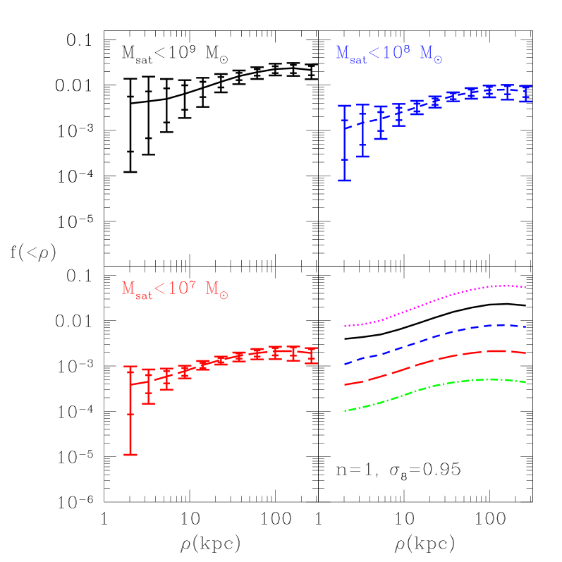
Figure 15: Mass fraction in substructure in cylindrical projection of radius $\rho$ for the same set of $n=1$ halos described in Figure 14. The upper left, upper right, and lower left panels show the mass fraction profiles in subhalos larger than $10^{6}$ M_⊙ and less than $10^{9}$, $10^{8}$ and $10^{7}$ M_⊙ respectively. Error bars reflect the same percentile ranges as do those in Figure 14. The bottom right panel illustrates how the mean projected mass fraction profiles vary as a function of the maximum subhalo mass considered: $10^{6.3}$, $10^{7}$, $10^{8}$, $10^{9}$, and $10^{10}$ M_⊙ from bottom to top.

The projected mass fractions are not as severely suppressed relative to the volume-averaged mass fractions as one might expect given that tidal forces act systematically to destroy substructure near host halo centers (see Figure 4). The reason is that we are examining substructure in a cylindrical volume, and picking up subhalos with large halo-centric radii. We illustrate this effect in Figure 14, where we compare the mass fraction in cylindrical projection radius $\rho$ with the mass fraction in spherical shells with the same value of spherical radius $r$. Notice that the mass fraction in spherical regions is significantly reduced in the center, while the projected mass fraction is less severely affected. Of course, the mass fraction approaches the global value at large radii. Figures 15 and 16 demonstrate how the mass fractions change as a function of projection radius for various subhalo mass cuts for the $n=1$ and BSI models respectively. Notice that the relative drop in mass fraction as a function of projection radius is more pronounced in the BSI model than in the $n=1$ case. This reflects the fact that tidal disruption is more important in the BSI case and core-like behavior of the subhalo radial distribution sets in at a larger radius in this model.

4.4 Warm Dark Matter and Gravitational Lensing

In the previous section we demonstrated that the substructure mass fraction is sensitive to abrupt changes in the power spectrum and used the BSI model as a specific example. In this section we investigate these differences in the context of WDM. We label the different WDM models by the warm particle mass $m_{\rm W}$, and assume the canonical case of a “neutrino-like” thermal relic with two internal degrees of freedom, $g_{\rm W}=2$.

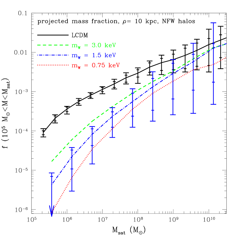
Figure 18: Cumulative mass fractions in substructure more massive than $10^{5}$ M_⊙ within a projected radius of $10$ kpc for the same models shown in Figure 17. The linetypes are the same as in Figure 17.

Figure 17 shows the total mass fraction of $3\times 10^{12}$ M_⊙ host halos at $z=0.6$ as a function of $M_{\rm sat}$ implied by our three WDM model power spectra compared to our standard $\Lambda$CDM case. For substructure smaller than $\sim 10^{7}$ M_⊙, the differences between the models are as large as an order of magnitude or more, and even the largest WDM particle mass ($3$ keV) provides a potentially measurable suppression of substructure. Figure 18 shows the mass fraction in projected cylinders of radius $10$ kpc.

The differences in mass fractions seen for the different models in Figures 17 and 18 come about because subhalos become less concentrated relative to their host halos as the WDM particle mass is decreased and power is suppressed on larger scales, much like the BSI case. In true WDM models there are additional processes that, in principle, can alter the formation and density structure of dark matter halos. In Figures 17 and 18, we have only accounted for the effect of the power spectrum on substructure mass fractions and assumed that the density structure of WDM halos is identical to that for CDM halos. For high mass systems, this is a sensible approximation (Colín et al. 2000a; Avila-Reese et al. 2001), but this approximation should break down at small masses and lead to further suppression of substructure.

One consequence of a WDM particle with non-negligible velocity dispersion is that gravitational clustering is resisted by structures below the effective Jeans mass of the warm particles (e.g., Hogan & Dalcanton 2000; Bode et al. 2001):

$$M_{\rm J}\approx 6\times 10^{3}\Bigg{(}\frac{{\rm keV}}{m_{\rm W}}\Bigg{)}^{4}\Bigg{(}\frac{\Omega_{\rm W}h^{2}}{0.15}\Bigg{)}^{1/2}\Bigg{(}\frac{2}{g_{\rm W}}\Bigg{)}(1+z)^{3/2}M_{\odot}.$$ (15)

For both the $m_{\rm W}=1.5$ keV and $m_{\rm W}=3.0$ keV models, $M_{\rm J}\ll 10^{5}M_{\odot}$ when $z\lower 2.58334pt\vbox{\hbox{$\buildrel\textstyle<\over{\sim}\ $}}10$, so all halos of interest in this context are minimally affected. The situation is somewhat more complicated in the $m_{\rm W}=0.75$ keV model, where $M_{\rm J}\lower 2.58334pt\vbox{\hbox{$\buildrel\textstyle>\over{\sim}\ $}}10^{5}$ M_⊙ for redshifts $z\lower 2.58334pt\vbox{\hbox{$\buildrel\textstyle>\over{\sim}\ $}}2$. We therefore expect that the formation of these halos should be suppressed compared to the predictions of the EPS formalism. This suppression should only have a minor effect on our predictions because we restrict ourselves to satellite masses $\lower 2.58334pt\vbox{\hbox{$\buildrel\textstyle>\over{\sim}\ $}}10^{5}$ M_⊙ and most surviving subhalos are accreted at $z\lower 2.58334pt\vbox{\hbox{$\buildrel\textstyle<\over{\sim}\ $}}2$. In the interest of simplicity, we chose to ignore this effect here. As a result, we may significantly over-predict substructure mass fractions at low $M_{\rm sat}$ in these cases. In the context of this study, this is a conservative approach because the true mass fraction would be reduced by these effects, bringing it further away from the measured substructure mass fractions and standard $\Lambda$CDM predictions.

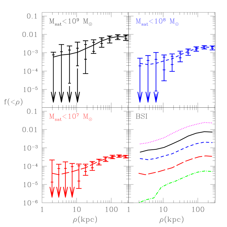
Figure 16: Mass fraction in substructure in cylindrical projection for the BSI model. All line types and panels are as described in Figure 15.

In addition to the effective Jeans suppression, WDM halos, unlike their CDM counterparts, cannot achieve extremely high densities in their centers due to phase space constraints (Tremaine & Gunn 1979). In the early Universe the primordial phase space distribution of the WDM particles is a Fermi-Dirac distribution with a maximum of $f_{\rm max}=g_{\rm W}/h_{\rm PL}^{3}$ at low energies ($h_{\rm PL}$ is Planck’s constant). For a collisionless species, the phase space density is conserved and this maximum phase space density may not be exceeded within WDM halos. If we define the phase density as $Q\equiv\rho/(2\pi\sigma^{2})^{3/2}$ then the maximum allowed phase density is (Hogan & Dalcanton 2000)

$$Q_{\rm max}\simeq 5.2\times 10^{-4}\Bigg{(}\frac{m_{\rm W}}{{\rm keV}}\Bigg{)}^{4}\Bigg{(}\frac{g_{\rm W}}{2}\Bigg{)}\ \frac{{\rm M}_{\odot}/{\rm pc}^{3}}{({\rm km}/{\rm s})^{3}}.$$ (16)

This limit implies that WDM halos cannot achieve the central density cusps of the kind observed in simulated CDM halos. Instead, we expect a core in the density profile. For viable WDM models, the phase space core is expected to be dynamically unimportant for any halo massive enough to host a visible galaxy (ABW). However, for the lowest-mass subhalos ($M\lower 2.58334pt\vbox{\hbox{$\buildrel\textstyle<\over{\sim}\ $}}10^{7}$ M_⊙) the presence of phase space-limited cores may be important because halos with large cores are less resistant to tidal forces than cuspy halos.

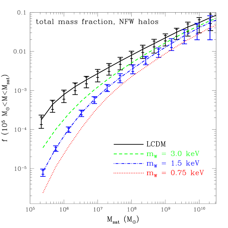
Figure 17: Total cumulative mass fractions in substructure more massive than $10^{5}$ M_⊙ for the $n=1$ and 3 WDM models. The models are $\Lambda$CDM (solid), $m_{\rm W}=3.0$ keV (dashed), $m_{\rm W}=1.5$ keV (dash-dot), and $m_{\rm W}=0.75$ keV (dotted). For clarity, we show error bars only for the $\Lambda$CDM and $m_{\rm W}=1.5$ keV models. The error bars and arrows have the same meaning as in Figure 13.

We have attempted to estimate (crudely) how the phase space limit affects the substructure population of WDM halos by adopting our standard model of halo accretion and orbital evolution, but allowing the density structure of the appropriately small subhalos to be set by the phase space limit. For these calculations we used the phenomenological density profile of Burkert (1995),

$$\rho_{\rm B}(r)=\frac{\rho_{0}}{[1+r/r_{\rm B}][1+(r/r_{\rm B})^{2}]}.$$ (17)

The Burkert profile resembles the NFW form at large radius, but features a constant density core at its center, and thus a velocity dispersion that approaches a constant at small $r$: $\sigma_{0}^{B}\simeq 0.55V_{\rm max}$. For Burkert profiles, $V_{\rm max}^{2}\simeq 0.86V_{\rm vir}^{2}c_{\rm B}/g_{\rm B}(c_{\rm B})$, where $c_{\rm B}\equiv R_{\rm vir}/r_{\rm B}$ is the Burkert concentration and $g_{\rm B}(y)\equiv\ln(1+y^{2})+2\ln(1+y)-2\tan^{-1}(y)$. Solving for the phase density in the core ($r\ll r_{\rm B}$) and equating it with the maximum phase density of equation (16) yields the following relation for the maximum attainable value of $c_{\rm B}$:

$$c_{\rm B}^{3/2}g_{\rm B}^{1/2}(c_{\rm B}) \simeq \frac{111}{(1+z)^{3}}\Bigg{(}\frac{0.15}{\Omega_{\rm W}h^{2}}\Bigg{)}\Bigg{(}\frac{178}{\Delta_{\rm vir}}\Bigg{)}\Bigg{(}\frac{V_{\rm vir}}{{\rm km/s}}\Bigg{)}^{3}$$ (18)

$$\times\Bigg{(}\frac{g_{\rm W}}{2}\Bigg{)}\Bigg{(}\frac{m_{\rm W}}{{\rm keV}}\Bigg{)}.$$

We assigned Burkert concentrations according to the following prescription. First, we computed NFW concentrations $c_{\rm vir}$, for each halo according to the B01 model. We converted from NFW concentration to Burkert concentration $c_{\rm B}$, by interpreting the B01 value of $r_{\rm s}$ as the radius at which $\textrm{d}\ln\rho(r)/\textrm{d}\ln r|_{r=r_{\rm s}}=-2$. This implies that $r_{\rm B}\simeq 0.66r_{\rm s}$ or $c_{\rm B}\simeq 1.5c_{\rm vir}$. With this correspondence, the adopted Burkert profile achieves the maximum of its rotation curve at $r_{\rm max}^{\rm B}\simeq 0.99r_{\rm max}$, where $r_{\rm max}$ is the radius at which the corresponding NFW halo achieves $V_{\rm max}$. Similarly, $V_{\rm max}$ of the adopted Burkert profile is within $10\%$ of the corresponding NFW $V_{\rm max}$ for all relevant concentrations ($1\leq c_{\rm vir}\leq 25$). Second, we computed the maximum value of $c_{\rm B}$ allowed by the phase space constraints using Eq. (18). We then assigned each halo the smaller of these two values of $c_{\rm B}$ at the time of accretion. In this way, we guaranteed that the phase space constraint was met by all halos. We have checked that this prescription for Burkert halos does not yield any systematic bias in our results by applying it all of our CDM models. We found that it gave nearly identical results to that of our standard NFW model, which is not surprising in the context of our model and disruption criteria.

We present our estimates of cumulative mass fractions in WDM models, including the effect of the phase space constraint, in Figure 19. It is clear, at least from this rough estimate, that the Tremaine-Gunn limit plays an important role only for the most extreme WDM models, $m_{\rm W}\lower 2.58334pt\vbox{\hbox{$\buildrel\textstyle<\over{\sim}\ $}}1$ keV, and only the smallest halos, $\lower 2.58334pt\vbox{\hbox{$\buildrel\textstyle<\over{\sim}\ $}}10^{6}$ M_⊙. However, we emphasize that our new assumptions about WDM halos have not been tested with N-body simulations. Simulations have yet to examine the density structure of halos that saturate the phase space bound and most studies have ignored the initial velocity dispersion of the WDM particles (Colín et al. 2000a; Avila-Reese et al. 2001, Knebe et al. 2002), but the Burkert profile assumption seems plausible. With these precautions in mind, Figure 17 may be regarded as an approximate upper-limit on the substructure mass fraction for WDM halos. Any phase space bound or the effects of primordial velocity dispersions on halo formation and density structure should lead to enhanced disruption, resulting in lower mass fractions.

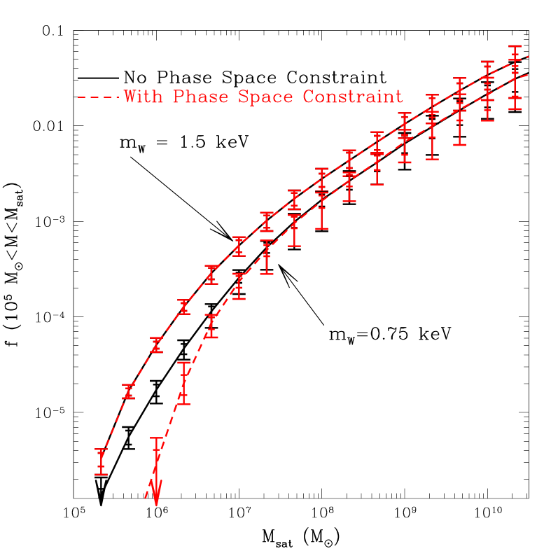
Figure 19: Total cumulative mass fractions in substructure more massive than $10^{5}$ M_⊙ both with (dashed) and without (solid) estimating the effects of the phase space limit. The upper set of lines corresponds to the $m_{\rm W}=1.5$ keV model and the lower set of lines corresponds to the $m_{\rm W}=0.75$ keV model. The error bars and arrows are as in Figure 13.

One physical process that might affect WDM (and BSI) models that we have not considered is top-down fragmentation (e.g., Knebe et al. 2002). It is possible that power can be transported from large scales to small in truncated models, resulting in a population of low-mass halos that would not be accounted for in Press-Schechter theory. While such a process could result in a higher substructure abundance than that estimated using our model, there are reasons to believe that the effect should be fairly small. Systems that form in this manner collapse quite late, and their density structure likely would be very diffuse compared to their hierarchically-formed brethren. Therefore, it is less likely that systems formed via fragmentation could survive tidal disruption once incorporated into a galactic halo.

4.5 The Dwarf Satellite Problem

Comparisons between the predicted subhalo population and the observed dwarf galaxy abundance are usually made by comparing counts as a function of maximum circular velocity, $V_{\rm max}$. This is a sensible mode of comparison because it sidesteps the complicated issues of star formation and feedback in these poorly-understood galaxies. Yet, there are considerable uncertainties, even for this method of comparison, and it is likely that efforts to compare predictions as a function of dwarf luminosity (Somerville 2002; Benson et al. 2002) in tandem with velocity comparisons will be needed in order to fully understand the nature of the dwarf satellite problem.

For most satellites, the quantity that is observed and used to infer the halo $V_{\rm max}$ is the line-of-sight stellar velocity dispersion, $\sigma_{\star}$. As discussed in S02 and H03, the mapping between $\sigma_{\star}$ and $V_{\rm max}$ depends upon the theoretical expectation for the density profile of the subhalo as well as on the stellar mass distribution of the galaxy. An additional complication concerns the unknown velocity anisotropy of the stars in the system.

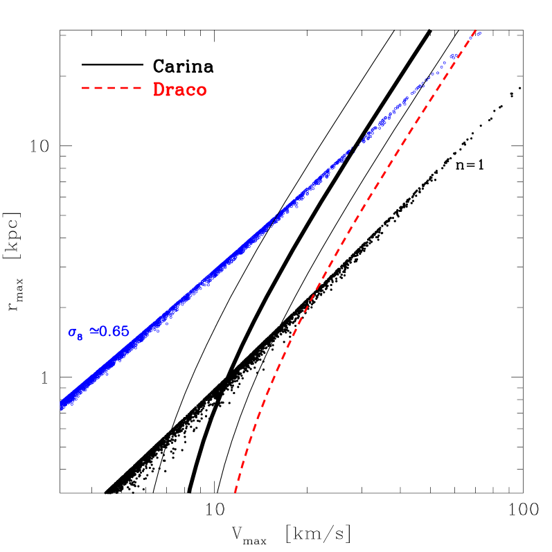
Figure 20: The lower and upper sets of points show a scatter plot of $V_{\rm max}$ and $r_{\rm max}$ for all surviving halos produced in 10 merger tree realizations for the $n=1$, and low-normalization, $\sigma_{8}=0.65$ models respectively. The thick solid line shows the locus of points in the $V_{\rm max}$-$r_{\rm max}$ plane that corresponds to the central value of the measured velocity dispersion of Carina ($\sigma_{\star}=6.8\pm 1.6\textrm{ km s}^{-1}$) given the measured King profile parameters of Carina (Table 2) and assuming NFW halos. The thin solid lines correspond to the $\pm 1\sigma$ quoted errors in velocity dispersion for Carina. The dashed line corresponds to the locus of points that is consistent with the central value of the measured velocity dispersion of Draco ($\sigma_{\star}=9.5\textrm{ km s}^{-1}$).

A phenomenologically-motivated approximation for the stellar distribution in a dwarf galaxy is the spherically symmetric King profile (King 1962),

$$\rho_{\star}(r)=\frac{k}{z^{2}}\Bigg{(}\frac{\cos^{-1}(z)}{z}-\sqrt{1-z^{2}}\Bigg{)},$$ (19)

where $z\equiv[1+(r/r_{\rm c})^{2}]/[1+(r_{\rm t}/r_{\rm c})^{2}]$, $r_{\rm c}$ and $r_{\rm t}$ are the core and tidal radii of the King profile, and $\rho_{\star}(r>r_{\rm t})=0$. The normalization is not important in what follows.

If we assume that a stellar system described by Equation (19) is in equilibrium and embedded in a spherically symmetric dark matter potential characterized by the circular velocity profile $V_{\rm c}(r)$, then the radial stellar velocity dispersion profile $\sigma_{\rm r}(r)$, can be computed via the Jeans equation:

$$r\frac{\textrm{d}[\rho_{\star}\sigma_{\rm r}^{2}]}{\textrm{d}r}=-\rho_{\star}(r)V_{c}^{2}(r)-2\beta(r)\rho_{\star}(r)\sigma_{\rm r}^{2}(r),$$ (20)

where the anisotropy parameter $\beta\equiv 1-\sigma_{\bot}^{2}/2\sigma_{r}^{2}$, $\sigma_{\bot}$ is the tangential velocity dispersion, and $\beta=0$ corresponds to an isotropic dispersion tensor. A measured, line-of-sight velocity dispersion is determined by the projected velocity dispersion profile weighted by the luminosity distribution sampled along the line-of-sight. For the isotropic case it is given by

$$\sigma_{\star}^{2}=\frac{\int_{0}^{r_{\rm t}}\rho_{\star}(r^{\prime})V_{\rm c}^{2}(r^{\prime})\textrm{d}r^{\prime}}{\int_{0}^{r_{\rm t}}\rho_{\star}(r^{\prime})\textrm{d}r^{\prime}},$$ (21)

assuming a constant mass-to-light ratio. If a galaxy has a measured stellar profile (the King parameters in this case) and measured value of $\sigma_{\star}$, then the Jeans equation places only one constraint on the rotation curve of the system, $V_{\rm c}(r)$. We expect the halo velocity profile to be at least a two-parameter function (e.g., the NFW profile) so determining $V_{\rm max}$ requires some theoretical input for the expected form of $V_{\rm c}(r)$ in order to provide a second constraint.

Motivated by dark matter models, we assume that the global rotation curve is set by an NFW profile associated with the dwarf galaxy halo. The rotation curve for an NFW halo is fully described by specifying two parameters and a natural pair is $V_{\rm max}$ and $r_{\rm max}$. For any given cosmology, the relation between $V_{\rm max}$ and $r_{\rm max}$ is expected to be rather tight, and this provides a second, theoretically-motivated constraint that sets the $V_{\rm max}$-$\sigma_{\star}$ mapping implied by Eq. (20).

The $V_{\rm max}$-$r_{\rm max}$ relationships for surviving subhalos in two of our models are shown in Figure 20. The lower set of points corresponds to our standard $n=1$ model and the higher set of points is derived from our $\sigma_{8}=0.65$ model. In each case, we plot one point for each surviving halo in 10 model realizations. The strong correlation, $r_{\rm max}\propto V_{\rm max}^{\gamma},\gamma\simeq 1.3$, follows directly from the input correlations between $M_{\rm vir}(z)$, and $c_{\rm vir}$ (see §2.3 and B01). The normalizations and slopes are influenced by the cosmology, accretion times and (mildly) by the orbital history of the subhalos.

The thick solid and dashed lines in Figure 20 show the locus of points in the $V_{\rm max}$-$r_{\rm max}$ plane that correspond to the central values of the observed line-of-sight velocity dispersions for Carina and Draco respectively, given their measured King profile parameters. Our adopted $\sigma_{\star}$ values and King parameters are listed in Table 2 along with appropriate references. The light solid lines illustrate how these contours expand when we include the $\pm 1\sigma$ measurement error in $\sigma_{\star}$ for Carina. A similar (although narrower) band exists for Draco, but we have omitted it for the sake of clarity. Consistency with the observed King parameters and velocity dispersions requires each dwarf to reside in a halo with structural parameters that lie within the region of overlap between the contours and the model points. For example, in the $n=1$ model Carina is expected to reside in a halo with $V_{\rm max}\approx 11\textrm{ km s}^{-1}$ and $r_{\rm max}\approx 1$ kpc. For the $\sigma_{8}=0.65$ model, Carina is expected to sit in a larger halo, with $V_{\rm max}\approx 29\textrm{ km s}^{-1}$ and $r_{\rm max}\approx 10$ kpc. Similar comparisons hold for Draco and all of the Local Group dwarf satellites and these comparisons can be made in a similar way for any cosmology. The point is that the maximum velocities that are assigned to satellite galaxies are cosmology-dependent. Therefore, “observed” velocity functions are also cosmology-dependent because theoretical inputs are used to convert from $\sigma_{\star}$ to $V_{\rm max}$.

In Table 2 we show estimates for halo $V_{\rm max}$ values for the observed Milky Way satellites under the assumption that $\beta=0$ along with a similar analysis for $\beta=0.15$ (values in parentheses). We estimate halo $V_{\rm max}$ values for six different power spectra, relying on the model-dependent $r_{\rm max}$-$V_{\rm max}$ relationship for substructure in each case, and taking the central values of the measured velocity dispersions for each halo. Taking the quoted $\pm 1\sigma$ range for the measured velocity dispersions typically leads to a shift in $V_{\rm max}$ of $\sim 30\%$ which is considerable compared to the inherent scatter in the $M_{\rm vir}-c_{\rm vir}$ relation. For reference, we have also included the adopted $V_{\rm max}$ values from the original K99 work on the dwarf satellite problem. As expected, the implied $V_{\rm max}$ values become larger as we explore models with less galactic-scale power. Our estimates for the $n=1$, $\beta=0$ case are close to those of K99.

The left panel of Figure 21 shows the Milky Way satellite counts for each model, assuming $\beta=0$, along with the predicted velocity functions for each model. In addition to the satellites listed in upper portion of Table 2, we have also included the Small Magellanic Cloud (SMC, with $V_{\rm max}=60\textrm{ km s}^{-1}$, estimated by Stanimirović 2000 to include a substantial contribution from the baryonic component) and the Large Magellanic Cloud (LMC, with $V_{\rm max}=50\textrm{ km s}^{-1}$, van der Marel et al. 2002) in our cumulative velocity functions. In the standard case ($n=1$) the discrepancy sets in at $V_{\rm max}\sim 30\textrm{ km s}^{-1}$, requiring roughly one-in-ten halos with $V_{\rm max}\sim 10-20\textrm{ km s}^{-1}$ to be the host of an observed galaxy. The extremely tilted model with $\sigma_{8}\simeq 0.65$ actually under-predicts the dwarf count for large systems. Interestingly, dwarfs in the ${\rm d}n/{\rm d}\ln k=-0.03$ RI model as well as the $\sigma_{8}=0.75$ case are consistent with inhabiting the ten most massive subhalos, with only Sextans standing as an outlier. The BSI model also looks to be in good agreement with the data for $V_{\rm max}\lower 2.58334pt\vbox{\hbox{$\buildrel\textstyle>\over{\sim}\ $}}12\textrm{ km s}^{-1}$, lending support to the conclusions of Kamionkowski & Liddle (2000). However, the problem of Local Group satellites is not completely “solved” in any of these models because the velocity function continues to rise below the velocity-scale of Sextans in all cases. What changes in the low-power models is the nature of the discrepancy. In one extreme, the mismatch sets in at $V_{\rm max}\sim 30\textrm{ km s}^{-1}$ and gradually becomes worse for smaller systems. In the other extreme, the mismatch seems to imply a sharp threshold for dwarf galaxy formation at a scale near $V_{\rm max}\sim 10-20\textrm{ km s}^{-1}$.

Unfortunately, a detailed accounting of the mismatch is difficult, even for a given cosmology. The dwarf $V_{\rm max}$ estimate is very sensitive to the velocity anisotropy parameter, $\beta$. For example, assuming $\beta=0.15$ leads to $V_{\rm max}$ values that are significantly lower than in the isotropic case because rotational support has been traded for pressure support. The velocity function comparisons with $\beta=0.15$ are shown in the right panel of Figure 21 and the $V_{\rm max}$ values are listed in parentheses in Table 2. In this case, only the $\sigma_{8}\simeq 0.65$ case and the BSI model can account for the dwarf population without a differential feedback mechanism. The rest of the models over-predict the counts, with the greatest apparent discord in the $n=1$ case. The specific choice of $\beta=0.15$ serves mainly to illustrate the effect of a minor anisotropy. We chose this value because it is typical of what is seen in the central regions of simulated dark matter halos (Colín et al. 2000b), and therefore it seems a reasonable possibility for the anisotropy parameter of particles in dwarf galaxies.

5 Caveats

In this study we employed a simple, semi-analytic model based on many previous studies (LC93; SK99; BKW; TB01; B01; W02; HFM02) and designed to produce large numbers of halo realizations with minimal computational effort. In developing this model, we have made many simplifying assumptions. In this section we draw attention to many of these shortcomings and discuss how they might affect our results and be improved upon in future work.

Among the most obvious omissions in this work is the neglect of any disk or bulge component in each halo. We have specifically chosen to ignore the effects of central galaxies because the physics of dark halo formation is relatively well-understood compared with that of galaxy formation. This allows us to ground our work against dissipationless N-body simulations. In order to include a galactic component, one is forced to adopt many poorly-constrained models and assumptions regarding gas accretion, cooling, angular momentum distributions, feedback, and the effects of substructure on the host galaxy itself. Once a reliable framework for the dark matter has been developed, we can use this as a foundation for more speculative (yet interesting) explorations involving the baryonic components.

A central (disk) galaxy would add to the dynamical friction force experienced by subhalos orbiting near the plane of the disk and cause halos on highly inclined orbits to be tidally heated during rapid encounters with the disk potential (e.g., Gnedin & Ostriker 1999; Gnedin, Hernquist, & Ostriker 1999; TB01). These effects lead to enhanced satellite disruption. Conversely, subsystems that are massive enough to host galaxies might be rendered more resistant to tidal disruption because their central densities would be enhanced by the presence of cool baryons. For low-mass halos, the net effect of a central galaxy would likely be to reduce the substructure count, mainly at small radii. Even without including these effects, we find that the substructure fraction drops significantly at small radii because of the dark matter potential, and that a large part of the projected central mass fraction comes from subhalos at large radii that are picked up in projection. Nevertheless, projected mass fractions are rather sensitive to the size of the core in the subhalo radial distribution (Chen et al. 2003), so if the core region were larger as a result of a central galaxy, the implied lensing signal would be reduced relative to our estimates. We find that eliminating all substructure within $20$ kpc of the halo center, reduces the projected mass fractions in subhalos less massive than $10^{10}$ M_⊙, $f_{10}$, by $\sim 30\%$.

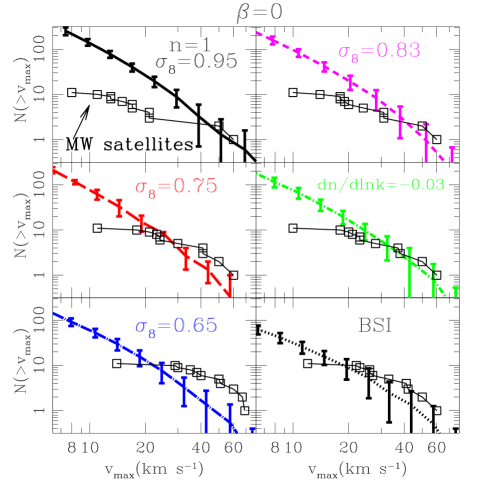
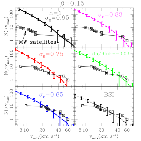
Figure 21: Satellite halo velocity functions for six of our models compared with the velocity functions of the Milky Way satellites after accounting for the cosmology-dependent mapping between $\sigma_{\star}$ and $V_{\rm max}$. The squares represent the velocity function of Milky Way satellites based on the data in Table 2. The lines represent the means over all realizations and the error bars reflect the dispersion among these realizations. The models are labeled in each panel.

Table 2: Characteristics of Milky Way satellites.

Satellite	$\sigma_{\star}$	$r_{c}$	$r_{t}$	$V_{\rm max}$	$V_{\rm max}$	$V_{\rm max}$	$V_{\rm max}$	$V_{\rm max}$	$V_{\rm max}$	$V_{\rm max}$
				K99	$n=1$	$\sigma_{8}=0.83$	RI model	$\sigma_{8}=.75$	BSI	$\sigma_{8}=0.65$
	($\textrm{ km s}^{-1}$)	(kpc)	(kpc)	($\textrm{ km s}^{-1}$)	($\textrm{ km s}^{-1}$)	($\textrm{ km s}^{-1}$)	($\textrm{ km s}^{-1}$)	($\textrm{ km s}^{-1}$)	($\textrm{ km s}^{-1}$)	($\textrm{ km s}^{-1}$)
Sagittarius	$11.7\pm 0.7$	0.44	3.0	20	17 (13)	20 (15)	23 (17)	24 (17)	26 (19)	35 (25)
Fornax	$10.5\pm 1.5$	0.46	2.3	18	15 (11)	18 (13)	20 (15)	21 (15)	23 (17)	30 (21)
Draco	$9.5\pm 1.6$	0.18	0.93	17	21 (15)	31 (20)	38 (25)	41 (26)	41 (29)	67 (44)
Ursa Minor	$9.3\pm 1.8$	0.20	0.64	16	21 (15)	31 (20)	37 (25)	41 (26)	42 (29)	69 (43)
Leo I	$8.8\pm 0.9$	0.22	0.82	15	17 (12)	24 (16)	28 (19)	30 (20)	33 (23)	51 (32)
Carina	$6.8\pm 1.6$	0.21	0.69	12	11 (8)	14 (10)	18 (13)	18 (13)	22 (16)	29 (19)
Leo II	$6.7\pm 1.1$	0.16	0.48	12	13 (9)	19 (13)	23 (16)	24 (16)	27 (19)	40 (26)
Sculptor	$6.6\pm 0.7$	0.11	1.5	11	13 (9)	18 (12)	21 (15)	23 (15)	26 (18)	38 (24)
Sextans	$6.6\pm 0.7$	0.34	3.2	11	8 (7)	10 (7)	10 (8)	11 (8)	12 (9)	14 (10)
SMC				30	$<60^{*}$	$<60^{*}$	$<60^{*}$	$<60^{*}$	$<60^{*}$	$<60^{*}$
LMC				50	50	50	50	50	$50^{*}$	$50^{*}$

Note. — The names of the satellite galaxies of the Milky Way are given in column (1). We consider only those galaxies with galactocentric distances smaller than $300$ kpc. Columns (2-4) give the measured line-of-sight velocity dispersion, and King core and tidal radii for each satellite. The exceptions are the LMC and the SMC. These galaxies have measured rotation speeds, listed in Columns (6-11). All velocities are expressed in units of $\textrm{ km s}^{-1}$ and distances are in kpc. Column (5) gives the value of $V_{\rm max}$ assigned to the halo of each satellite by by K99. Columns (6-11) and above the horizontal space give the value of $V_{\rm max}$ that we estimated for each satellite based on its measured velocity dispersion and King profile parameters and assuming the primordial power spectra specified at the top of each column. Values of $V_{\rm max}$ listed without parentheses were calculated assuming an anisotropy parameter of $\beta=0$, and those inside parentheses assume $\beta=0.15$. Except for the case of Draco, we use the velocity dispersions and King profile core and tidal radii for the Milky Way satellites given in the review article by Mateo (1998). For Draco, we use the parameters quoted by Odenkirchen et al. (2001). The quoted maximum rotation speeds for the LMC and SMC were taken from van der Marel et al. (2002) and Stanimirović (2000). The LMC rotation curve is observed to be flat from $4$kpc out to $>8.9$kpc. For many of the low-power models (indicated by superscript “^∗”), the flat portion of the curve ($\sim r_{\rm max}$) is expected to be at larger radius. In order to explain this in the context of these models, we must suppose that baryonic in-fall plays an important role in setting the properties of dark matter rotation curves (Blumenthal et al. 1986). In this case, the measured value of $V_{\rm max}$ ($r_{\rm max}$) is larger (smaller) than it would be for the pristine halo prior to baryonic contraction. The SMC rotation curve is even more likely to be influenced by baryons (Stanimirović 2000), and baryonic in-fall is likely to be of some importance for all cases. While not demanded by the data, the effects of baryonic in-fall could be important for all satellites, thus the listed $V_{\rm max}$ values should be considered lower limits. Lastly, the large value of $r_{\rm max}$ associated with Draco in the $\sigma_{8}=0.65$ case may be difficult to reconcile with the kinematic data of Kleyna et al. (2002) and may disfavor a model with such low power.

In addition to the considerable uncertainties associated with galaxy formation, there are potential shortcomings in our efforts to model substructure properties in the context of collisionless dark matter physics alone. For example, we have allowed for only a mild redistribution of mass within the tidal radii of the orbiting subhalos up until the time the subhalo is totally disrupted. The work of S02 and H03 suggests that this effect may be larger, but these results may have been compromised by limited numerical resolution or inappropriate assumptions regarding initial subhalo orbits and/or accretion times. In this sense, our approach represents a conservative extreme because we assume that the surviving subhalo density structure is typically very similar to that of halos in the field. We study the effects of tidal mass redistribution in a forthcoming paper (J. Bullock, K. Johnston, & A. Zentner, in preparation). In addition, we have adopted a halo concentration relation (B01) that has not been confirmed for $M\lower 2.58334pt\vbox{\hbox{$\buildrel\textstyle<\over{\sim}\ $}}10^{9}$ M_⊙. Similarly, the EPS merger tree calculations have yet to be tested in the very low-mass regime. In light of these extrapolations, it is imperative that our results be tested, and updated using the next generation of numerical studies.

Finally, our model does not treat the substructure population self-consistently. We have neglected any subhalo-subhalo interactions which could serve to increase the internal heating of substructure and modify dynamical friction timescales as orbital energy is exchanged between subhalos and traded for internal energy. We have adopted the approximation that all in-falling halos are “distinct” and have no subhalos of their own (see Taylor & Babul 2003 for a study of merger tree “pruning”). However, our “tree-level” calculations suggest that the substructure mass fraction is uniformly $\sim 10\%$ regardless of host mass, so we expect the that this correction would typically affect our derived mass fractions by $\lower 2.58334pt\vbox{\hbox{$\buildrel\textstyle<\over{\sim}\ $}}10\%$. Considering the assumptions that have gone into our calculations and the current level of observational precision, this level of error is acceptable; however, it may need to be improved upon as observations zero in on the masses of the subclumps responsible for the lensing signals and the mass fractions in these subclumps.

6 Conclusions and Discussion

The abundance of substructure in dark matter halos is determined by a continuous competition between accretion and disruption. Accreted subhalos with dense cores are resistant to disruption, but over time their orbits decay, their mass is stripped away, and they are often destroyed. The model we presented here allows us to follow the complicated interplay between density structure, orbital evolution, and accretion time in order to determine how changes in the power spectrum affect the final substructure population in galaxy-sized halos. For a fixed set of cosmological parameters, changes in the power spectrum manifest themselves by changing collapse times for halos, where less power leads to later accretion times and lower densities. We have specifically focused on tilted models that help to relieve the central density crisis facing CDM and that may be favored by joint CMB and large-scale structure analyses (Spergel et al. 2003). We have also considered a BSI inflation model and WDM models, where the power is sharply reduced on small scales.

For a large class of CDM-type models, including models with significant tilt and running, we find that the fraction of mass bound up in substructure $f$, for galaxy-mass halos is relatively insensitive to the slope of the primordial power spectrum. This is because both the host halos and their accreted subsystems collapse later in these models, in a roughly self-similar way as power is reduced. Note that this result would have been roughly expected if we were varying only the overall normalization in the models because the relative redshifts of collapse would be invariant (we assume host halos are small enough that they collapse before $z\sim 0$). Our investigation suggests that this intuitive description holds even for tilted and running index models, at least over the parameter range we have explored. All indications are that this insensitivity to the tilt of the power spectrum is a rather robust result, and should hold even if some unknown factor has caused our overall normalization in predicted mass fractions to be in error (e.g., our exclusion of central galaxies). Interestingly, the shape of the mass function, $f(x\equiv M_{\rm sat}/M_{\rm host})$, is also relatively insensitive to the mass of the host halo [Eq. (14)], and a similar shape holds for all of the tilted models we explored.

The similarity in mass fractions breaks down for models with sharp features in their power spectra, like our BSI and WDM models. In these models, low-mass halo formation is delayed significantly relative to the formation time of their hosts. Consequently, fewer subhalos are dense enough to withstand the tidal field they experience upon accretion. We find that for the relevant WDM and BSI models, the mass fraction in substructure is reduced by a factor of $\lower 2.58334pt\vbox{\hbox{$\buildrel\textstyle>\over{\sim}\ $}}3$ compared to the standard/tilted $\Lambda$CDM models.

Inspired by recent attempts to measure substructure mass fractions using multiply-imaged quasars, we applied our model to ensembles of host halos with $M=3\times 10^{12}$ M_⊙ at $z=0.6$, which represents the expectation for massive lens galaxies (DK01; DK02). For the $\Lambda$CDM/tilted cases, we found substructure mass fractions within a $10$ kpc projected radius in systems less massive than $M=10^{8}$, $10^{9}$, and $10^{10}$M_⊙ of $f_{8}\simeq 0.2-0.4\%$, $f_{9}\simeq 0.4-1.5\%$, and $f_{10}\simeq 0.6-2.5\%$ at the $64$ percentile range. These estimates are consistent with, but on the low side of, first attempts to measure the substructure fraction using multiply-imaged quasars by DK01, who obtain $f\simeq 0.6\%-7\%$ at $90\%$ confidence, with an upper-mass limit of $10^{8}-10^{10}$ M_⊙ (N. Dalal, private communication). The lensing results disfavor the BSI model, which leads to mass fractions $f_{8}\simeq 0.01-0.06\%$, $f_{9}\simeq 0.02-0.2\%$, and $f_{10}\simeq 0.03-0.4\%$ at $64$%. This is true unless the break scale in the power spectrum is pushed to such a small value that this model no longer has the attractive feature of alleviating the central density problem. A $m_{\rm W}=0.75$ keV WDM model is similarly disfavored, and even our highest mass WDM case, $m_{\rm W}=3$ keV, has a typical projected fraction ($f_{9}\sim 0.4\%$) that is low compared to the DK01 estimate. Again, this indicates that if the warm particle is a thermal relic, the mass must be large enough that WDM no longer mitigates the small-scale problems of standard CDM. Yet, these results are interesting because they show how lensing may be used as one of the few probes of the WDM particle mass in the range $\lower 2.58334pt\vbox{\hbox{$\buildrel\textstyle>\over{\sim}\ $}}1$ keV or a break in the primordial power spectrum at large wavenumber.

Clearly these conclusions must be regarded with some caution. In addition to the uncertainties of modeling discussed in §5, other issues make drawing definite conclusions difficult. For example, we have only accounted for the substructure within the virial radius of the host halo, yet the anomalous flux ratios of lensed images are sensitive to the presence of small halos along the line-of-sight to the lens. Keeton (2003) showed that field halos can have a significant lensing effect even if they are separated from the lens by several tenths in redshift and in hierarchical, CDM-type models, small field halos are ubiquitous. Chen et al. (2003) showed that the relative effect from halos outside the virial radius of the lens is typically a few percent, but may be as large as $20-30\%$ of that from subhalos, depending upon assumptions about the subhalo population. Also, as the mass fraction in substructure of a given mass depends on the mass of the host [Eq. (14)], it may be important to constrain the host halo mass in order to fully exploit the ability of lensing measurements of substructure to probe cosmology and structure formation.

We compared our model predictions for the cumulative subhalo velocity function, $N(>V_{\rm max})$, to the satellite galaxy count of the Milky Way. The approach here was to estimate $V_{\rm max}$ for each satellite galaxy’s dark matter halo based on its observed line-of-sight velocity dispersion, $\sigma_{\star}$. We emphasized in §4.5 that the mapping between $\sigma_{\star}$ and $V_{\rm max}$ is sensitive to theoretical prejudice regarding the density structure of the dwarf galaxy’s halo as well as the unknown velocity anisotropy parameter of the system, $\beta$. For a fixed value of $\beta$, less concentrated host halos imply larger values of $V_{\rm max}$ because halo rotation curves are more slowly rising and stars probe only the inner $\sim 1$ kpc of the halo. Interestingly, this implies that tilted models and truncated models, do significantly better than $n=1$, $\Lambda$CDM in reproducing apparent dwarf counts, even though their mass fractions are similar. While our estimates of $V_{\rm max}$ cannot be considered robust because of the simplicity of our model and the fact that the $\sigma_{\star}-V_{\rm max}$ mapping is very sensitive to the inner structure of the subhalos, the general trends that we illustrate should persist in more elaborate studies and N-body simulations. Moreover, our results reveal yet another reason why it is difficult to consider the dwarf satellite problem a serious challenge to CDM theory, the nature of the dwarf satellite problem is very sensitive to cosmology, the power spectrum, and assumptions about the shape of the velocity ellipsoid for stars in dwarf galaxies.

When we fix $\beta=0$, our ${\rm d}n/\rm{d}\ln k=-0.03$ RI model, $\sigma_{8}=0.75$ model, and the BSI case all do well in matching the known satellite population of the Milky Way for $V_{\rm max}\lower 2.58334pt\vbox{\hbox{$\buildrel\textstyle>\over{\sim}\ $}}20\textrm{ km s}^{-1}$. Our lowest power model ($\sigma_{8}=0.65$, $n\simeq 0.84$, and mild running) actually under-predicts the dwarf count for $V_{\rm max}\lower 2.58334pt\vbox{\hbox{$\buildrel\textstyle>\over{\sim}\ $}}$ 30$\textrm{ km s}^{-1}$. However, this result is achieved only for the optimistic assumption of isotropic velocities. If we adopt a small level of anisotropy, $\beta=0.15$, consistent with the centers of simulated dark matter halos, agreement for most models is worsened. Only the BSI and $\sigma_{8}=0.65$ models show good agreement in this case. Yet, even with $\beta=0.15$, the RI and $\sigma_{8}=0.75$ models still compare more favorably than the $n=1$ case with $\beta=0$.

What do these results imply for the dwarf satellite problem? In all models, including those with truncated power, the velocity function of subhalos continues to rise below the scale of the smallest observed Milky Way satellite, $V_{\rm max}\lower 2.58334pt\vbox{\hbox{$\buildrel\textstyle<\over{\sim}\ $}}10\textrm{ km s}^{-1}$. No matter how one modifies the power spectrum, some kind of feedback is required to explain the local satellite population. Different power spectra (even different values of $\beta$) seem to indicate that different types of feedback are needed. For example, in models with $\sigma_{8}\lower 2.58334pt\vbox{\hbox{$\buildrel\textstyle>\over{\sim}\ $}}0.8$ (the precise number depends on typical $\beta$ values and the degree of running/tilt), the feedback must be differential. That is, for $V_{\rm max}\simeq 8-30\textrm{ km s}^{-1}$, only one out of every $\sim 5-10$ halos in this range should form stars. On the other hand, in models like the ${\rm d}n/{\rm d}\ln k=-0.03$ RI model, the BSI case, and our $\sigma_{8}\simeq 0.75$ model with $\beta=0$, the discrepancy seems to set in suddenly at $V_{\rm max}\sim 10-20\textrm{ km s}^{-1}$, suggesting that nearly all halos smaller than this are completely devoid of stars. In this case, the feedback mechanism must provide a sharp transition.

The feedback mechanism proposed by BKW accommodates the need for only $\sim 10\%$ of subsystems to actually host observable galaxies by suggesting that only those systems that formed before reionization were able to retain their gas and eventually form stars. However, if reionization were to occur very early (e.g., $z\lower 2.58334pt\vbox{\hbox{$\buildrel\textstyle>\over{\sim}\ $}}15$), many fewer than $10\%$ of these dwarf-sized systems could have collapsed before reionization, so that almost all systems smaller than $V_{\rm max}\sim 30\textrm{ km s}^{-1}$ would be dark. This would be more in line with what we see for the low-power models. This is an intriguing result. The best-fit power spectrum of the WMAP team (Spergel et al. 2003) leads to similar substructure mass fractions as standard CDM, alleviates the central density problem and dwarf satellite discrepancy, and forces us to consider feedback mechanisms that predict a sharp transition between luminous and non-luminous galaxies. Additionally, the possible detection of early reionization by the WMAP team (Kogut et al. 2003) provides a feedback mechanism that results in a sharp transition. Of course, explaining early reionization in models with low small-scale power may be problematic (Somerville et al. 2003). Another feedback scenario that leads to a sharp transition is photo-evaporation (Barkana & Loeb 1999; Shaviv & Dekel 2003). Nonetheless, the uncertainty associated with $\beta$ in determining satellite galaxy $V_{\rm max}$ values suggests that efforts to model dwarf galaxy luminosities as well as dynamical properties will be required to resolve this issue (Somerville 2002; Benson et al. 2002).

Remaining uncertainties in understanding the precise nature of the dwarf satellite problem highlight the need to focus on attempts to measure CDM substructure by other means. Continued efforts to detect substructure via gravitational lensing (e.g., DK01; Keeton 2003; Keeton, Gaudi, & Petters 2002; Moustakas & Metcalf 2003) or by probes within our own Galaxy (e.g., Johnston et al. 2002; Ibata et al. 2002a, 2002b; Mayer et al. 2002; Font et al. 2001) offer useful avenues for doing so. Modeling of the kind presented here may play an important role in interpreting results of ongoing observational programs and bring us one step closer to confirming or refuting one of the fundamental predictions of the CDM paradigm.

References

- (1) Alam, S. M. K., Bullock, J. S., & Weinberg, D. H. 2002, ApJ, 572, 34 (ABW)
- (2) Allen, S. W., Schmidt, R. W., Fabian, A. C., & Ebeling, H. 2002, MNRAS, in press
- Avila-Reese et al. (2001) Avila-Reese, V., Colín, P., Valenzuela, O., D’Onghia, E., & Firmani, C. 2001, ApJ, 559, 516
- (4) Avila-Reese, V., Firmani, C. & Hernández, X. 1998, ApJ, 505, 37
- (5) Bahcall, N. A. et al. 2003, ApJ, 585, 182
- (6) Bahcall, N. A. & Bode, P. 2003, ApJL, 588, L1
- (7) Bardeen, J. M., Bond, J. R., Kaiser, N., & Szalay, A. 1986, ApJ, 304, 15
- (8) Barkana, R., Haiman, Z., & Ostriker, J. P. 2001, ApJ, 558, 482
- Barkana & Loeb (1999) Barkana, R. & Loeb, A. 1999, ApJ, 523, 54
- (10) Bennett, C. L. et al. 1994, ApJL, 464, L1
- (11) Benson, A. J., Frenk, C. S., Lacey, C. G., Baugh, C. M., & Cole, S. 2002, MNRAS, 333, 177
- (12) Binney, J. J. & Evans, N. W. 2001, MNRAS, 327, 27
- Blumenthal, Faber, Primack, & Rees (1984) Blumenthal, G. R., Faber, S. M., Primack, J. R., & Rees, M. J. 1984, Nature, 311, 517
- (14) Blumenthal, G. R., Faber, S. M., Flores, R., & Primack, J. R. 1986, ApJ, 301, 27
- Bode, Ostriker, & Turok (2001) Bode, P., Ostriker, J. P., & Turok, N. 2001, ApJ, 556, 93
- (16) Bond, J. R., Cole, S., Efstathiou, G., & Kaiser, N. 1991, ApJ, 379, 440
- (17) Borgani, S. et al. 2001, ApJ, 561, 13
- (18) Borriello, A. & Salucci, P. 2000, MNRAS, 323, 285
- Bradač et al. (2002) Bradač, M., Schneider, P., Steinmetz, M., Lombardi, M., King, L. J., & Porcas, R. 2002, A&A, 388, 373
- (20) Brown, M. L., Taylor, A. N., Bacon, D. J., Gray, M. E., Dye, S., Meisenheimer, K., & Wolf, C. 2002, MNRAS, 341, 100
- (21) Bryan, G. L. & Norman, M. L. 1998, ApJ, 495, 80
- (22) Bullock, J. S., Kravtsov, A. V., & Weinberg, D. H. 2000, ApJ, 539, 517, (BKW)
- Bullock, Kravtsov, & Weinberg (2001) Bullock, J. S., Kravtsov, A. V., & Weinberg, D. H. 2001, ApJ, 548, 33
- (24) Bullock, J. S., Kolatt, T. S., Sigad, Y., Somerville, R. S., Kravtsov, A. V., Klypin, A. A., Primack, J. R., & Dekel, A. 2001, MNRAS, 321, 559, (B01)
- (25) Bunn, E. F., Liddle, A. R., & M. White 1996, Phys. Rev. D, 54, 5917R
- (26) Bunn, E. F., & White, M. 1997, ApJ, 480, 6
- (27) Burkert, A. A. 1995, ApJL, 447, L25
- (28) Chandrasekhar, S. 1943, ApJ, 97, 255
- Chen, Kravtsov, & Keeton (2003) Chen, J., Kravtsov, A. V., & Keeton, C. R. 2003, ApJ, 592, 24
- CGO (01) Chiu, W. A., Gnedin, N. Y., & Ostriker, J. P. 2001, ApJ, 563, 21
- (31) Cole, S., Aragon-Salamanca, A., Frenk, C. S., Navarro, J. F., & Zepf, S. E. 1994, MNRAS, 271, 781
- Colín, Avila-Reese, & Valenzuela (2000) Colín, P., Avila-Reese, V., & Valenzuela, O. 2000a, ApJ, 542, 622
- Colín, Klypin, & Kravtsov (2000) Colín, P., Klypin, A. A., & Kravtsov, A. V. 2000b, ApJ, 539, 561
- Colín, Klypin, Kravtsov, & Khokhlov (1999) Colín, P., Klypin, A. A., Kravtsov, A. V., & Khokhlov, A. M. 1999, ApJ, 523, 32
- (35) Colombi, S., Dodelson, S., & Widrow, L. M. 1996, ApJ, 458, 1
- (36) Colpi, M., Mayer, L., & Governato, F. 1999, ApJ, 525, 720
- (37) Côte, S., Carignan, C., & Freeman, K. C. 2000, AJ, 120, 3027
- (38) Covi, L. & Lyth, D. H. 1999, Phys. Rev. D, 59, 063515
- (39) Covi, L., Lyth, D. H., & Roszkowski, L. 1999, Phys. Rev. D, 60, 023509
- (40) Covi, L., Lyth, D. H., & Melchiorri, A. 2003, PRD, 67, 043507
- (41) Croft, R. A. C., Weinberg, D. H., Katz, N., & Hernquist, L. 1998, ApJ, 495, 44
- (42) Croft, R. A. C, Weinberg, D. H, Bolte, M., Burles, S., Hernquist, L., Katz, N., Kirkman, D., & Tytler, D. 2002, ApJ, 581, 20
- (43) Dalal, N. & Kochanek, C. S. 2001, ApJ, 572, 25 (DK01)
- (44) Dalal, N. & Kochanek, C. S. 2002, PRL, submitted (astro-ph/0202290) (DK02)
- Dalcanton & Bernstein (2002) Dalcanton, J. J. & Bernstein, R. A. 2002, AJ, 124, 1328
- (46) Debattista, V. P. & Sellwood, J. A. 2000, ApJ, 543, 704
- (47) de Blok, W. J. G., McGaugh, S., & Rubin, V. C. 2001, AJ, 122, 2396
- (48) de Blok, W. J. G. & Bosma, A. A. 2002, A&A, 385, 816
- Dekel & Woo (2002) Dekel, A. & Woo, J. 2002, MNRAS, submitted (astro-ph/0210454)
- (50) Dekel, A. & Silk, J. 1986, ApJ, 303, 38
- (51) Efstathiou, G. 1992, MNRAS, 256, 43P
- (52) Eisenstein, D. J. & Hu, W. 1999, ApJ, 511, 5
- Eke, Navarro, & Frenk (1998) Eke, V. R., Navarro, J. F., & Frenk, C. S. 1998, ApJ, 503, 569
- Eke, Navarro, & Steinmetz (2001) Eke, V. R., Navarro, J. F., & Steinmetz, M. 2001, ApJ, 554, 114 (ENS)
- (55) Font, A. S., Navarro, J. F., Stadel, J., & Quinn, T. 2001, ApJL, 563, L1
- (56) Ghigna, S., Moore, B., Governato, F., Lake, G., Quinn, T., & Stadel, J. 1998, MNRAS, 300, 146
- (57) Ghigna, S., Moore, B., Governato, F., Lake, G., Quinn, T., & Stadel, J. 2000, ApJ, 544, 616
- Gnedin (2000) Gnedin, N. Y. 2000, ApJ, 542, 535
- (59) Gnedin, O. Y. & Ostriker, J. P. 1999, ApJ, 513, 626
- (60) Gnedin, O. Y., Hernquist, L. & Ostriker, J. P. 1999, ApJ, 514, 109
- (61) Hamana, I. et al. 2002, ApJ, submitted (astro-ph/0210450)
- (62) Hashimoto, Y., Funato, Y., & Makino, J. 2002, ApJ, 582, 196 (HFM02)
- (63) Hayashi, E., Navarro, J. F., Taylor, J. E., Stadel, J., & Quinn, T. 2003, ApJ, 584, 541, (H03)
- Hodges & Blumenthal (1990) Hodges, H. M. & Blumenthal, G. R. 1990, Phys. Rev. D, 42, 3329
- Hogan & Dalcanton (2000) Hogan, C. J. & Dalcanton, J. J. 2000, Phys. Rev. D, 62, 063511
- (66) Ibata, R. A., Lewis, G. F., Irwin, M. J., & Quinn, T. 2002a, MNRAS, 332, 915
- (67) Ibata, R. A., Lewis, G. F., Irwin, M. J., & Cambrésy, L. 2002b, MNRAS, 332, 921
- (68) Jarvis, M., Bernstein, G., Fischer, P., Smith, D., Jain, B., Tyson, J. A., & Wittman, D. 2003, AJ, 125, 1014
- (69) Jing, Y. 2000, ApJ, 535, 20
- (70) Johnston, K. V. 1998, ApJ, 495, 297
- (71) Johnston, K. V., Spergel, D. N., & Haydn, C. 2002, ApJ, 570, 656
- (72) Kamionkowski, M. & Liddle, A. R. 2000, Phys. Rev. Lett., 84, 4525
- (73) Kauffmann, G., White, S. D. M., & Guiderdoni, B. 1993, MNRAS, 264, 201
- (74) Keeton, C. R. 2001, ApJ, 561, 46
- (75) Keeton, C. R. 2003, ApJ, 584, 664
- (76) Keeton, C. R., Gaudi, B. S., & Petters, A. O. 2002, ApJ, submitted (astro-ph/0210318)
- (77) King, I. 1962, AJ, 67, 471
- (78) Kleyna, J., Wilkinson, M. I., Evans, N. W., Gilmore, G., & Frayn, C. 2002, MNRAS, 330, 792
- (79) Klypin, A. A, Kravtsov, A. V., Valenzuela, O., & Prada, F. 1999a, ApJ, 522, 82 (K99)
- Klypin, Gottlöber, Kravtsov, & Khokhlov (1999) Klypin, A., Gottlöber, S., Kravtsov, A. V., & Khokhlov, A. M. 1999b, ApJ, 516, 530
- Klypin, Zhao, & Somerville (2002) Klypin, A., Zhao, H., & Somerville, R. S. 2002, ApJ, 573, 597
- Knebe, Devriendt, Mahmood, & Silk (2002) Knebe, A., Devriendt, J. E. G., Mahmood, A., & Silk, J. 2002, MNRAS, 329, 813
- (83) Kochanek, C. S. & Dalal, N. 2003, ApJ, submitted
- (84) Kogut, A. et al. 2003, ApJ, submitted
- Kolatt et al. (1999) Kolatt, T. S. et al. 1999, ApJ, 523, L109
- (86) Komatsu, E. & Seljak, U. 2002, MNRAS, 336, 1256
- (87) Kosowsky, A. & Turner, M. S. 1995, Phys. Rev. D, 52, 1739
- Kravtsov (1999) Kravtsov, A. V. 1999, Ph.D. Thesis,
- (89) Lacey, C. & Cole, S. 1993, MNRAS, 262, 627, (LC93)
- (90) Lin, W. B., Huang, D. H., Zhang, X., & Brandenberger, R. 2001, Phys. Rev. Lett., 86, 954
- (91) Mac Low, M.-M. & Ferrara, A. 1999, ApJ, 413,142
- (92) Marchesini, D., D’Onghia, E., Chincarini, G., Firmani, C., Conconi, P., Molinari, E., & Zacchei, A. 2002, ApJ, 575, 801
- (93) Mateo, M. 1998, ARA&A, 36, 435
- (94) Mayer, L., Moore, B., Quinn, T., Governato, F., & Stadel, J. 2002, MNRAS, 336, 119
- (95) McDonald, P. V., Miralda-Escudé, J., Rauch, M., Sargent, W. L. W., Barlow, T. A., Cen, R., & Ostriker, J. P. 2000, ApJ, 543, 1
- (96) McGaugh, S. S., Barker, M. K., & de Blok, W. J. G. 2003, ApJ, 584, 566
- (97) Melchiorri, A. & Silk, J. 2002, PRD, 66, 014301
- Metcalf (2002) Metcalf, R. B. 2002, ApJ, 580, 696
- Metcalf & Zhao (2002) Metcalf, R. B. & Zhao, H. 2002, ApJ, 567, L5
- Metcalf & Madau (2001) Metcalf, R. B. & Madau, P. 2001, ApJ, 563, 9
- (101) Moore, B., Ghigna, S., Governato, F., Lake, G., Quinn, T., Stadel, J., & Tozzi, P. 1999a, ApJL, 524, L19
- (102) Moore, B., Quinn, T., Governato, T., Stadel, J., & Lake, G. 1999b, MNRAS, 310, 1147
- Moustakas & Metcalf (2003) Moustakas, L. A. & Metcalf, R. B. 2003, MNRAS, 339, 607
- (104) Narayan, V. K., Spergel, D. N., Davé, R., & Ma, C.-P. 2000, ApJL, 543, L103
- (105) Navarro, J. F., Frenk, C. S. & White, S. D. M. 1997, ApJ, 490, 493, (NFW)
- (106) Odenkirchen, M. et al. 2001, AJ, 122, 2538
- Pagels & Primack (1982) Pagels, H. & Primack, J. R. 1982, Phys. Rev. Lett., 48, 223
- (108) Peiris, H. V. et al. 2003, ApJ, in press (astro-ph/0302225)
- (109) Percival, W. J. et al. 2002, MNRAS, 337, 1068
- (110) Pierpaoli, E., Borgani, S., Scott, D., & White, M. 2002, MNRAS, 342, 163
- (111) Power, C., Navarro, J. F., Jenkins, A., Frenk, C. S., White, S. D. M., Springel, V., Stadel, J., & Quinn, T. 2003, MNRAS, 338, 14
- Quillen & Garnett (2001) Quillen, A. C. & Garnett, D. R. 2001, ASP Conf. Ser. 230: Galaxy Disks and Disk Galaxies, 87 (astro-ph/0004210 )
- (113) Quinn, T., Katz, N., & Efstathiou, G. 1996, MNRAS, 278, L49
- Rees (1986) Rees, M. J. 1986, MNRAS, 218, 25P
- (115) Schuecker, P., Böhringer, H., Collins, C. A., & Guzzo, L. 2002, A & A, 398, 867
- Seljak, McDonald, & Makarov (2003) Seljak, U., McDonald, P. V., & Makarov, A. 2003, MNRAS, in press (astro-ph/0302571)
- (117) Shapiro, P. R., Giroux, M. L., & Babul, A. 1994, ApJ, 427, 25
- (118) Shaviv, N. & Dekel, A. 2003, MNRAS, submitted (astro-ph/0305527)
- Shetrone, Côté, & Sargent (2001) Shetrone, M. D., Côté, P., & Sargent, W. L. W. 2001, ApJ, 548, 592
- Somerville & Primack (1999) Somerville, R. S. & Primack, J. R. 1999, MNRAS, 310, 1087
- (121) Somerville, R. S. & Kolatt, T. S. 1999, MNRAS, 305, 1, (SK99)
- (122) Somerville, R. S. 2002, ApJ, 572, 23
- Somerville, Bullock, & Livio (2003) Somerville, R. S., Bullock, J. S., & Livio, M. 2003, ApJL, sumbitted (astro-ph/0303481)
- Spergel et al. (2003) Spergel, D. N. et al. 2003, ApJ, in press (astro-ph/0302209)
- Stanimirović (2000) Stanimirović, S. 2000, Ph.D. Thesis, (http://astron.berkeley.edu/ sstanimi/)
- (126) Starobinsky, A. A. 1992, JETP Lett., 55, 489
- (127) Stewart, E. D. 1997a, Phys. Lett. B, 391, 34
- (128) Stewart, E. D. 1997b, Phys. Rev. D, 56, 2019
- (129) Stoehr, F., White, S. D. M., Tormen, G., & Springel, V. 2002, MNRAS, 335, L84, (S02)
- (130) Swaters, R. A. 1999, Ph.D. Thesis
- (131) Swaters, R. A., Madore, B. F., van den Bosch, F. C., & Balcells, M. 2003, 583, 732
- (132) Taylor, J. E. & Babul, A. 2001, ApJ, 559, 716, (TB01)
- (133) Taylor, J. E. & Babul, A. 2002, preprint (astro-ph/0210074)
- (134) Taylor, J. E. & Babul, A. 2003, MNRAS, submitted (astro-ph/0301612)
- (135) Thoul, A. A. & Weinberg, D. H. 1996, ApJ, 465, 608
- (136) Tremaine, S. & Gunn, J. E. 1979, PRL, 42, 407
- (137) Turner, M. S. 2002, Int. J. Mod. Phys., A17, 3446
- Valenzuela & Klypin (2003) Valenzuela, O. & Klypin, A. 2003, American Astronomical Society Meeting, 201, #51.01
- (139) van den Bosch, F. C. & Swaters, R. 2001, MNRAS, 325, 1017
- (140) van den Bosch, F. C., Mo, H. J., & Yang, X. 2003, MNRAS, submitted (astro-ph/0301104)
- van der Marel, Alves, Hardy, & Suntzeff (2002) van der Marel, R. P., Alves, D. R., Hardy, E., & Suntzeff, N. B. 2002, AJ, 124, 2639
- (142) Van Waerbeke, L., Mellier, Y., Pello, R., Pen, U.-L., McCracken, H. J., Jain, B. 2002, A&A, 393, 369
- Verde et al. (2003) Verde, L. et al. 2003, ApJ, in press (astro-ph/0302218)
- (144) Viana, P. T., Nichol, R. C., & Liddle, A. R. 2002, ApJ, 569, 75
- (145) von Hoerner, S. 1957, ApJ, 125, 451
- (146) Wechsler, R. H., Bullock, J. S., Primack, J. R., Kravtsov, A. V., & Dekel, A. 2002, ApJ, 568, 52, (W02)
- (147) White, S. D. M. 1976, MNRAS, 174, 467
- (148) White, S. D. M. & Rees, M. J. 1978, MNRAS, 183, 341
- (149) White, S. D. M. 1996, in Cosmology and Large-Scale Structure, ed. R. Schaeffer, J. Silk, & J. Zinn-Justin (Dordrecht: Elsevier Science)
- (150) Zaroubi, S. & Hoffman, Y. 1993, ApJ, 416, 410
- (151) Zentner, A. R. & Bullock, J. S. 2002, Phys. Rev. D, 66, 043003, (ZB02)