The interstellar oxygen-K absorption edge as observed by XMM-Newton

High resolution X-ray spectra of the Reflection Grating Spectrometer (RGS) on board the XMM satellite are used to resolve the oxygen K absorption edge. By combining spectra of low and high extinction sources, the observed absorption edge can be split in the true interstellar (ISM) extinction and the instrumental absorption. The detailed ISM edge structure closely follows the edge structure of neutral oxygen as derived by theoretical R-matrix calculations. However, the position of the theoretical edge requires a wavelength shift. In addition the detailed instrumental RGS absorption edge structure is presented. All results are verified by comparing to a subset of Chandra LETG-HRC observations.

1 Introduction

In the past, detectors in the low energy (0.3 - 2.0 keV) X-ray band offered spectra of modest spectral resolution. To properly model these spectra, equivalent spectral resolution knowledge of the oxygen K-edge absorption was required in order to correct the intrinsic source spectra for the effects of interstellar extinction. With the appearance of high resolution X-ray spectrographs, notably the XMM-Newton RGS (den Herder et al. herder (2001)) and Chandra LETG (Brinkman et al. brinkman (2000)), the ISM oxygen K-edge absorption can be studied in much greater detail. These instruments, however, usually suffer from absorption by oxygen located within the instruments. By comparing spectra from sources with low and high extinction and assuming that the interstellar cross-section per hydrogen atom is constant over the sky, the instrumental and interstellar components can be separated.

Models of extinction in X-rays by the interstellar medium have been constructed, amongst others, by Morrison and McCammon (morrison (1983)). These models are based on assumed abundance’s of the ISM and cross sections by Henke et al. (henke (1982)). However, the spectral resolution in current spectrographs surpasses the resolution of the Henke tables.

For neutral atomic oxygen far more detailed absorption cross sections have been calculated by the R-matrix approach (McLaughlin and Kirby, matrix (1998)). These cross sections include all the fine structure resonance’s along the K edge (around 22.6 - 22.9 Å), including the 1s-2p transition at approximately 23.5 Å. Neutral oxygen is thought to be the major constituent of the ISM. Therefore, a good model of the detailed spectral structure around the oxygen K edge can be constructed by combining the “R-matrix” cross sections of neutral oxygen with the Morrison and McCammon extinction cross sections for the remaining elements. The ISM oxygen abundance as presented by Wilms et al. (wilms (2000)) is used. Fig. 1 shows the combined cross section.

In the matrix calculations uncertainties of up to 3.5 eV, or 0.15 Å are reported for certain energy levels which can lead to shifted absolute positions of the resonance structures. The relative structure however, which gives rise to the detailed shape of the observed edge, can be expected to be known with much higher accuracy. The theoretical bound-bound resonance’s wavelengths (e.g. the 1s-2p line) were shifted to be in agreement with laboratory data, such that for these transitions the error can be expected to be less.

Of course interstellar oxygen can also be present in other forms then neutral atoms. Ionised oxygen can be expected and oxygen can be bound in molecules (e.g. OH, CO, $\rm{H}_{2}\rm{O}$), either as free gases, or as a solid component of interstellar dust (e.g. ice, silicates). Although the X-ray signature of ionised oxygen is well known, the X-ray signature of bound oxygen is much harder to identify. Depending on the detailed chemical and crystal structure and the presence and structure of other compounds, the X-ray spectral signatures may shift by up to 5 % (chemical shift, see e.g. Sevier, sevier (1979)), and can be broadened. For this reason the exact X-ray absorption spectrum of interstellar dust is not really known. Since neutral atomic oxygen is believed to be the most significant constituent of interstellar oxygen it is therefore justified to include its X-ray absorption features only in our interstellar oxygen model.

Figure 1: Theoretical cross sections for the ISM around the oxygen K edge based on the R-matrix (McLaughlin and Kirby, matrix (1998)) computations for neutral atomic oxygen combined with the Morrison and McCammon (morrison (1983)) profile for other elements. The edge is not infinitely sharp, but consists of a series of resonance features, indicated in the plot. The well known 1s-2p transition feature is also indicated.

In this paper we derive the shape of the interstellar oxygen absorption edge by comparing the absorption features in sources with low and high extinction. We compare the neutral oxygen model cross sections with the derived shape of the spectral profiles of interstellar extinction observed by the RGS, corrected for the instrumental response. Possible deviations from the model will be discussed in terms of the presence or upper limits of other oxygen components. In addition the detailed features of the RGS instrumental absorption are resolved. A subset of Chandra measurements is used to crosscheck the results obtained.

2 Data

To study spectral absorption features of the oxygen K edge, a number of bright sources with simple intrinsic (power law) spectra and no obvious narrow spectral features, were selected. Table 1 lists the sources. The corresponding XMM-Newton orbits of the RGS data and Chandra observation ID’s of the LETG data are shown, as well as the $N_{\rm{H}}$ ISM column densities used.

Since the main features in our spectra are caused by oxygen, we also show the oxygen column density based on the ISM abundance by Wilms et al. (wilms (2000)). For the extragalactic sources (Mrk~421, PKS~2155-304, 3C~273) we checked that we got reasonable agreement with the oxygen spectral features, starting from the $N_{\rm{H}}$ columns from an independent source (Kaastra, kaastra (2002)), while for the galactic sources (Sco-X1 and 4U0614+091) we actually fitted the oxygen column and convert to $N_{\rm{H}}$. It may be noted that for the derivation of the actual shape of the interstellar oxygen edge the precise oxygen column densities of the individual sources are irrelevant.

Finally, for comparison only, we add the $N_{\rm{H}}$ column densities based on H i radio surveys. Since the line of sight towards the galactic sources is likely to cross galactic molecular material, a correction for the presence of $\rm{H}_{2}$ based on a ratio of $\rm{H}_{2}$ to H i of 0.3 (Dame et al. dame (1987)) is applied. For Sco-X1 we assume all observed H i to be in front of the source, since its distance of 2.8 kpc (Bradshaw et al. bradshaw (1999)) and galactic latitude of about 24 degrees places it well above the scale height of $\approx$ 150 pc of H i in the galaxy. For 4U~0614+091 a wide variety of distances is reported (see Brandt et al., brandt (1992)) from 2 to 8 kpc although an upper limit of 3 kpc seems likely. Combined with the low galactic latitude for this source of only 3 degrees, makes the estimated H i column highly uncertain.

Despite some uncertainties in the H i column densities, table 1 shows quite good agreement between our $N_{\rm{H}}$ columns derived from X-ray data and the H i columns. This is a strong indication that the absorption is truly interstellar and not originating at the source. This means the absorption characteristics can be assumed similar for all our sources.

On the RGS the oxygen edge is covered by CCD detector 4. Unfortunately, early in the mission the CCD4 chain on RGS2 failed. As a consequence the oxygen data for on-axis sources originate from the single CCD chip on RGS1 only. The bad spots (warm or hot pixels) on this CCD detector 4 cause large systematic uncertainties in the spectra so these regions have to be omitted from the analysis. These bad spots usually occur at the same wavelength for one source, but could be slightly shifted for a different source, due to small differences in source position with respect to the telescope axis. By combining the spectra of the low extinction sources Mrk~421 and PKS~2155-304 the effect of these bad spots is reduced significantly due to slight differences in the relative pointings of these sources.

Table 1: Overview of sources and basic data

	Observation		exposurei	$N_{\rm{H}}$ column	$N_{\rm{O}}$ columna	$N_{\rm{H}}$ from H i
Source	XMM-Newton b	Chandra c	(ksec)	($\times 10^{20}\rm{cm}^{-2}$)	($\times 10^{17}\rm{cm}^{-2}$)	($\times 10^{20}\rm{cm}^{-2}$)
Mrk~421	84,171,259		172	$1.66\pm 0.09^{\mathrm{d}}$	$0.85\pm 0.04$	$1.61\pm 0.10^{\mathrm{e}}$
PKS~2155-304	87,174,362	3166	346	$1.25\pm 0.08^{\mathrm{d}}$	$0.65\pm 0.04$	$1.36\pm 0.10^{\mathrm{e}}$
3C~273	277		90	$1.76\pm 0.10^{\mathrm{d}}$	$0.90\pm 0.05$	$1.68\pm 0.10^{\mathrm{e}}$
Sco-X1	224,402		12	$20.0\pm 1.5^{\mathrm{f}}$	$10.2\pm 0.8$	$19.0\pm 3^{\mathrm{g}}$
4U~0614+091	231	100	23	$31.\pm 4.^{\mathrm{h}}$	$15.9\pm 0.4$	$28\pm 10^{\mathrm{g}}$

• Derived from the $N_{\rm{H}}$ column depth based on the oxygen ISM abundance’s from Wilms, Allen and McCray (wilms (2000))

• XMM-Newton orbit number.

• Chandra Obs-ID.

• Taken from independent Chandra data (Kaastra, kaastra (2002))

• Based on H i observations by Lockman and Savage (lockman (1995)).

• Fitted on the RGS data (this paper).

• Based on the H i survey by Hartmann and Burton (hartmann (1997)) and a ratio of $\rm{H}_{2}$ to H i of 0.3 (Dame et al, dame (1987)). The errors are based on local gradients in the H i map and uncertainties in source distances.

• Based on fits in both the Chandra and RGS data (this paper).

• Total RGS exposure time

For the “high extinction” source Sco-X1 a different approach was adopted. Sco-X1 is sufficiently bright to allow large offset pointings (of about 27 arcmin.) which shifted the oxygen edge to CCD detector 3 (orbit 402). Since both CCD3 detectors are active on both RGS’s, redundancy between the two CCD3 detectors solves the problem with bad positions on the detector corresponding to a particular wavelength range. Comparing the individual CCD3 spectra and an additional on-axis pointing on Sco-X1 with the oxygen edge on CCD4 (orbit 224) it was confirmed that the instrumental oxygen edge is identical for the different detector chips, which implies that the same instrumental profile applies irrespective of the location of the Oxygen edge on the instrument.

The data of 3C~273 were used as an independent check to verify that the derived instrumental absorption profile for the RGS is correct.

In all figures in this paper data are fluxed spectra, corrected for exposure and the effective area excluding of course the effects of instrumental oxygen absorption. Error bars represent the $1\sigma$ statistical error.

The lower effective area and limited exposure times of Chandra imply higher statistical noise compared with XMM. Including the Chandra observations however, enables an independent check of the derived properties of the interstellar oxygen absorption. All Chandra data shown are corrected for the overlapping $2^{\rm{nd}}$ and $3^{\rm{rd}}$ orders.

3 RGS analysis

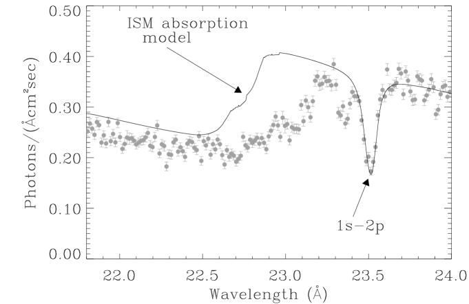
Figure 2: RGS spectrum around the oxygen K edge of Sco-X1 (grey data points). The solid black line represents the theoretical interstellar absorption (Fig. 1) convolved with the RGS instrumental resolution for an ISM column density of $N_{\rm{H}}=2.0\times 10^{21}\rm{cm}^{-2}$. The ISM 1s-2p absorption feature is also indicated.

Fig. 2 shows the RGS spectrum around the oxygen K edge for Sco-X1. Overplotted is the theoretical profile based on the cross sections of Fig. 1, convolved with the RGS instrument response and using an extinction column depth of $N_{\rm{H}}=2.0\times 10^{21}\leavevmode\nobreak\ \rm{cm}^{-2}$. With this column depth the 1s-2p absorption line fits the data after applying a 30 mÅ shift of the theoretical position to longer wavelengths. This is somewhat larger than expected based on the known accuracy of the RGS wavelength scale of $1\sigma=8$ mÅ (den Herder et al., herder (2001)).

Figure 3: Relation between equivalent line width of the 1s-2p absorption and $N_{\rm{O}}$ column density. The solid lines show the curves for neutral oxygen for different velocity dispersions of 10, 30 and 100 km/s from the lowest to the highest solid line respectively. Curves for velocities $\leq$ 10 km/s overlap with the lowest curve (10 km/s). The broken lines show the same for singly ionised oxygen (O ii).

Due to the very high optical depth of the narrow 1s-2p line core, saturation effects can be expected. Given the cross sections of the 1s-2p line as shown in Fig. 1, the expected relation between equivalent width of the line and the column density was computed for a variety of velocity dispersions. This is shown in Fig. 3. The bend in the curves for high column density does indicate saturation effects, but due to the broad wings in the line (contrary to e.g. lines of O i in the UV), the equivalent width of the line keeps increasing steadily even for high optical depths. This means that even for high extinction the column density can be reasonably well determined from the equivalent width. However, the actual equivalent width and depth of the observed line profile do depend on the velocity dispersion along the line of sight. Entering realistic velocity dispersions ($<$ 200 km/s) did not improve the fit sufficiently to allow for tight constraints on the velocity dispersion and column depth. Therefore a fit of the 1s-2p line only, leaves a rather large uncertainty on the actual column density. Fixing the column depth to $N_{\rm{H}}=2.0\times 10^{21}\leavevmode\nobreak\ \rm{cm}^{-2}$ and performing more detailed modeling of the 1s-2p line depth using the SPEX package (Kaastra, 2002c ) points to a velocity dispersion in the range of 30 - 50 km/s. However, this is highly dependent on the real distribution of the velocity components. In addition, given the errors on the equivalent widths (Table 2) and too poor resolution of the RGS for this purpose, the fitted velocity dispersion can only be seen as an indication only.

Since the depth of the absorption below the edge (below 22.5 Å) is a measure for the total of ISM and instrumental extinction, it was checked whether the difference between ISM absorption model and data below the edge can be attributed to the instrument. The depth of the instrumental oxygen absorption determined later in this paper, does indeed match this offset. Since the depth of the absorption below the edge extends over a large wavelength range and is therefore not influenced by ISM velocity dispersions, it is believed that the current fit does give a good measure of the true oxygen column depth for this source. The derived column density is also in good agreement with the numbers retrieved from H i observations (see Table 1).

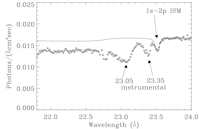
Figure 4: RGS combined spectrum around the oxygen K edge for the low extinction sources (Mrk~421, PKS~2155-304). A fit of the theoretical ISM absorption model to the 1s-2p line at 23.5 Å is also shown (black line). Main difference with the data points is due to the additional instrumental absorption. Two key instrumental features at 23.05 and 23.35 Å are indicated.

Fig. 4 shows the RGS spectrum for the sum of Mrk~421 and PKS~2155-304 data. This is the “low extinction” data. Of course this summed spectrum yields a kind of weighted average of the spectral characteristics of the two individual objects Mrk~421 and PKS~2155-304. Since we are not interested in the intrinsic source spectra the large scale shape of the combined spectrum is not relevant. The $N_{\rm{H}}$ column depth for both sources is low and does not differ too much between the sources. It is therefore estimated that the distortion of the ISM absorption profile due to adding the two sources is well within the statistical uncertainty of the individual data points.

For these “low extinction” data, the model wavelengths are shifted by 35 mÅ to longer wavelengths to fit the 1s-2p feature. This shift is consistent with the 30 mÅ shift in Fig. 2 given the 8 mÅ  error on the RGS wavelength scale. Main difference between the data points of these low extinction sources and the overplotted ISM absorption is due to the additional instrumental absorption. Two key instrumental features can be clearly recognised at around 23.05 and 23.35 Å. This is the fingerprint of the actual compounds in the instrument which cause the absorption. These dips can also be noticed in Fig. 2, in the Sco-X1 data. The fact that the equivalent width of the 23.35 feature (see Table 2) is the same for both Sco-X1 and the low extinction sources, despite the fact that the $N_{\rm{H}}$ column densities differ more than a factor of 10, does confirm the instrumental nature of this feature.

Taking the ratio between the “low” and “high” extinction data will remove all the features which are constant between the data, in particular the instrumental features. What is left must represent the true interstellar extinction. This ratio is shown in Fig. 5 (black data points).

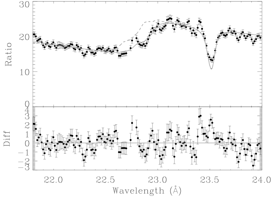
Figure 5: Ratio of the spectra of Figs. 2 and 4 (black data points). This represents the variable interstellar extinction between the sources. The broken grey line shows the fitted theoretical extinction. The solid grey line shows this theoretical extinction with the edge shifted by 0.13 Å. Error bars shown represent the $1\sigma$ statistical error.

The theoretical ISM extinction curve (broken grey line) is fitted to the depth of the edge below 22.5 Å. By comparing the theoretical oxygen edge with the extinction data, it appears that the shape of the edge matches the data, but that the position of the edge is shifted. The solid grey line shows this effect. It is identical to the broken line but with the edge (all the resonance structures identified with the indicated edge in Fig. 1) shifted by 0.13 Å, to larger wavelengths. The error uncertainty of this shift is estimated at 0.02 Å. Hereafter, we use these absorption cross sections with shifted oxygen edge as our model of the interstellar oxygen K edge.

It shows clearly in Fig. 5 that the absorption dips around 23.05 and 23.35 Å, which are present in both the low and high extinction data (Figs. 2 and 4) have largely disappeared in the ratio plot, which indicates that both features are generated by the RGS instrument itself. Possible residues deviate less than $3\sigma$ from the model.

Any deviations in Fig. 5 from the model can point to absorption features of other components, in particular other forms of oxygen. Any amount of oxygen, either atomic, in molecules or solid compounds will be reflected by the depth of the oxygen edge. Therefore the depth of the edge by itself cannot separate different components. Oxygen compounds other then the neutral atomic form can only be seen if they show distinct, sufficiently narrow, absorption features. In order to judge possible strengths of other absorption features, the level of the fitted continuum is important. In Fig. 5 it shows that the continuum is very well constrained by the data below 22.5 Å and above 23.7 Å. Although fit residues between 22.5 and 23.5 Å seem to suggest additional structure, the tight constraints on the continuum level do not allow much freedom to move the continuum up to a higher level such that there is room for clear absorptions. Taking into account the error on the fitted continuum, the fit residues can be analysed in terms of upper limits on possible other oxygen compounds.

A striking feature in the fit residue is the feature around 22.77 Å. At this wavelength some excess flux appears in the ratio plot (Fig. 5), which means that this feature is not present in the Sco-X1 data (Fig. 2). Inspection of the individual XMM data show that this feature is present in both Mrk~421 and PKS~2155-304 data but not in the 4U 0614+91 and Sco-X1 spectra. The spectrum of the combined low extinction sources, Fig. 6 shows this feature as a clear distinct absorption feature. It is unlikely that the apparent excess flux in the ratio plot is caused by two absorption dips on both sides of the 22.77 Å feature, e.g. due to solid ISM oxygen compounds. In that case the Sco-X1 should have shown the 22.77 Å feature in “emission” as well. In the subsequent section we will show that the Chandra data of PKS~2155-304 and 4U 0614+91 show the same behaviour as the RGS data. For this reason this feature is attributed to the PKS~2155-304 and Mrk~421 source spectra.

If we tentatively identify this feature (Fig. 6) in the PKS~2155-304 and Mrk~421 spectra with an O iv absorption blend at 22.75 Å, given the equivalent width of $\approx 10$mÅ, we derive a column density of $N_{{O\textsc{iv}}}$ of $6\times 10^{15}\rm{cm}^{-2}$. The most likely candidate for this absorption is the local filament as observed e.g. in O vii by Nicastro et. al. (nicastro (2002)), with a column density of $4\times 10^{15}\rm{cm}^{-2}$. However, since Nicastro et. al. derive an O vi column of only $0.1\times 10^{15}\rm{cm}^{-2}$, the O iv is most likely due to a less ionised component. If the gas is photo ionised, we expect O iv to peak at $\rm{log}\xi\simeq-0.8$. For this ionization parameter the column density of the neighbouring O iii and O v ions is a factor of 3 smaller than the O iv column and we estimate the strongest spectral features of those ions to be at 22.33 Å(O v, eq. width = 4 mÅ) and 23.08 Å(O iii, eq. width = 2 mÅ). Equivalent widths of this order of magnitude are not completely excluded by the data, taking into account that these lines positions are uncertain by about $\approx 0.03$ Å. Unfortunately, there is no clear positive indication of these lines.

Looking in detail to other features in the fit residues of the ratio spectrum of Fig. 5, features can be recognized at 23.05 and 23.35 Å. The 23.05 Å feature seems an incomplete cancellation of the 23.05 Å instrumental feature and has an equivalent width of $3\pm 3$ mÅ. Finally there seems some structure around 23.35 Å which has an equivalent width of $4\pm 3$ mÅ. A tentative explanation could be traces of O iii (at 23.05 Å) and O ii (at 23.35 Å). This implies column densities of $\approx 5\times 10^{15}\rm{cm}^{-2}$ (see Fig. 3). All these column densities are sufficiently low, such that their combined K-edge has an optical depth less than 0.01. This puts constraints on the average ionization stage of oxygen in the interstellar medium. Higher ionization stages of Oxygen may dominate the hotter components of the interstellar medium.

Apart from possible lines of ionised oxygen, oxygen locked in solids may cause features in the fit residues of Fig. 5. It is well known that in solids the spectral features of X-ray absorption lines can be shifted (see e.g. Sevier, sevier (1979)) and broadened with respect to the corresponding lines in free atoms. For broader lines saturation effects are less critical. If the combined features identified above would be attributed to shifted and broadened 1s-2p lines of neutral oxygen in solid compounds, we estimate the amount of oxygen in these features at less than 10 % of the neutral oxygen. In case of possible saturation effects the estimated upper limits will become smaller. If however the combined chemical shifts of lines of oxygen locked in solids smear out its signature over a broad wavelength band, its signature will be completely lost and large amounts of oxygen may be hidden in solids which are simply not detected by X-ray absorption features.

The fact that the depth of the 1s-2p line does not quite match the data is not really relevant. As explained before, the relative depths of the edge and the line of the high extinction component in the ratio data is rather arbitrary and depends on other factors (ISM velocity field) then just the column depth of the absorbing material.

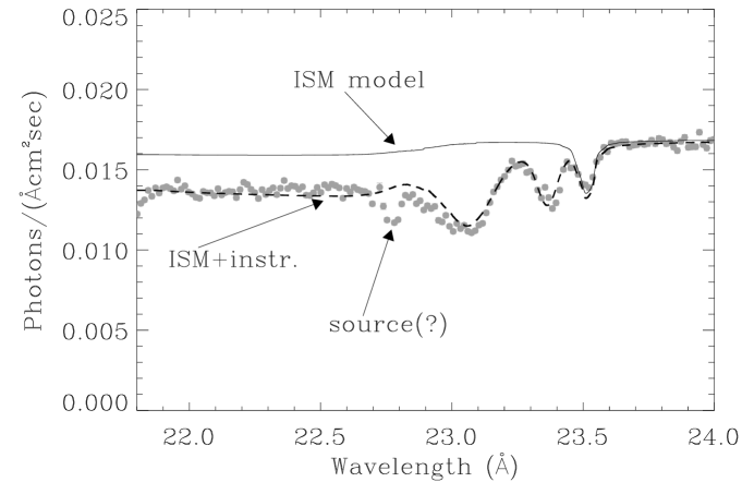
Figure 6: Fit of modified 1s-2p lines to the instrumental features for the low extinction data (Fig. 4). The broken line shows the combination of our interstellar extinction model (black line) and the fit of a broadened shifted atomic 1s-2p line model to the 23.05 and 23.35 Å instrumental features.

If the instrumental features at 23.05 and 23.35 Å are interpreted as shifted 1s-2p lines of bound oxygen in some solid compounds located on the detectors or optics, the column density for these features can be fitted. First our interstellar extinction model is fitted to the interstellar 1s-2p line of the low extinction data at 23.5 Å(Fig. 6). Fig. 3 shows that for the fitted ISM column density of $N_{\rm{H}}=1.5\leavevmode\nobreak\ \times\leavevmode\nobreak\ 10^{20}\leavevmode\nobreak\ \rm{cm^{-2}}$, which corresponds to $N_{\rm{O}}=0.76\leavevmode\nobreak\ \times\leavevmode\nobreak\ 10^{17}\leavevmode\nobreak\ \rm{cm^{-2}}$, line saturation effects are minor and only uncertainty in velocity dispersion will influence the determined column density. We assumed velocity dispersions $\leq 10$ km/s for these high galactic latitude sources.

In addition to this ISM absorption the instrumental 23.05 and 23.35 Å features are fitted by shifting and broadening the 1s-2p line. It now appears that with this instrument model the depth of the edge below 22.5 Å is also well fitted. This is interpreted as a confirmation that the 23.05 and 23.35 Å features are indeed shifted and broadened 1s-2p lines. The oxygen column density in both instrumental features amounts to $N_{\rm{O}}=2.5\pm 0.2\leavevmode\nobreak\ \times 10^{17}\leavevmode\nobreak\ \rm{cm}^{-2}$. If all this instrumental oxygen would be in the form of water(ice) only, this column density amounts to a layer of about $750\pm 50$ Å thickness. However, the fact that we see two features might indicate that the oxygen is present in two different compounds.

The actual difference in Fig. 6 between the fitted theoretical interstellar extinction curve and the data (ignoring the 22.77 Å  feature) can be interpreted as the instrumental oxygen absorption. For these low extinction sources, any uncertainty in the exact shape of the interstellar oxygen edge, whether or not features of other forms of oxygen then just neutral oxygen are present, hardly plays a role. The derived corresponding efficiency of the RGS instrument is plotted in Fig. 7. This efficiency is implemented in the current calibration files (CCF) for the RGS response, used by the XMM SAS data reduction software package (Jansen et al. jansen (2001)). Note that some of the sharp “edges” in the graph result from the fitting process used to derive the instrumental curves. They have no physical meaning. These sharp features disappear when this correction is applied to the instrument response.

Figure 7: The derived instrumental efficiency due to the instrumental oxygen absorption. The extrapolations beyond the wavelength range of 21.8 - 24.0 Å have been derived from the Henke (henke (1982)) tables (broken lines).

Our interstellar and instrumental absorption models around the oxygen K edge were verified by applying them to 3C~273. The statistical and systematic (due to warm/hot columns in the RGS CCDs) noise is higher for this data than the datasets used above. Using a column depth of $N_{\rm{H}}=1.76\times 10^{20}\leavevmode\nobreak\ \rm{cm}^{-2}$, derived from independent Chandra data, yields an acceptable fit to these data (Fig. 8).

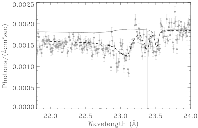
Figure 8: Fit of our interstellar model with a column depth of $N_{\rm{H}}=1.76\times 10^{20}\rm{cm}^{-2}$ and our instrumental efficiency model to the RGS spectrum of 3C~273 in the wavelength range around the oxygen K edge

4 Cross checking on Chandra data

The method to compare data from low and high extinction sources to derive absorption characteristics of the ISM can also be applied to Chandra data. We looked at a subset of Chandra LETG HRC data, since this Chandra grating/detector combination has the highest effective area at the oxygen K-edge. The observations are listed in Table 1.

Fig. 9 shows the Chandra observation of the low extinction source PKS~2155-304. Comparing with the XMM-RGS observation of the low extinction sources in Fig. 4 it is immediately apparent that the deep instrumental absorption feature seen at 23.05 Å in the XMM data is largely absent in the Chandra data. The 23.35 Å instrumental absorption feature however can be recognised in the Chandra data. This feature is treated similarly as for the XMM-RGS, by assuming it to be a shifted/broadened instrumental 1s-2p line. This fit is shown with the plotted broken line. Also the suspected absorption due to the source at 22.77 Å can be recognised in the Chandra data.

From these observations it follows that the general instrumental absorption characteristics between Chandra-LETG-HRC and XMM-RGS differ, but the 23.35 Å component is common in both instruments.

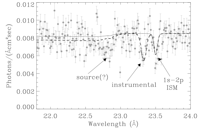
Figure 9: Chandra LETG HRC observation of PKS~2155-304. The solid black line represents the ISM absorption using our $N_{\rm{H}}$ of $1.25\times 10^{20}\rm{cm}^{-2}$. The broken line shows a fit to the instrumental line at 23.35 Å which can also be recognised in the XMM-RGS data. Here, this fit corresponds to an oxygen column depth of $8\times 10^{16}\rm{cm}^{-2}$. The feature at 22.77 Å, which is also seen in the XMM-RGS is attributed to the source itself.

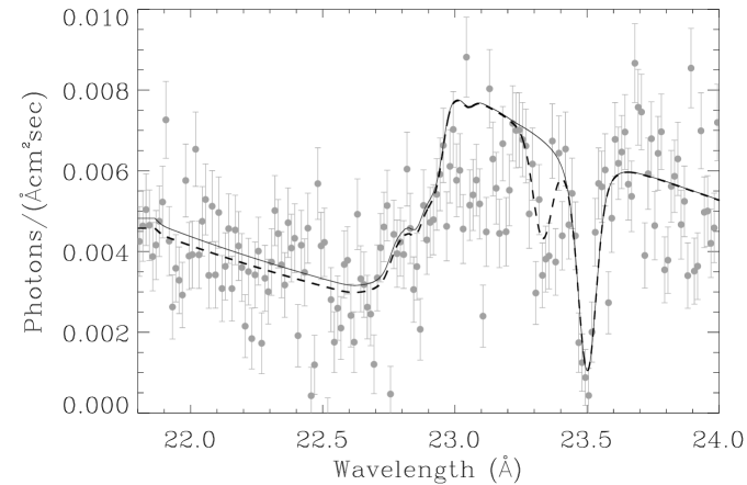
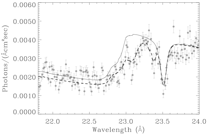
Figure 10: Chandra LETG HRC observation of 4U~0614+091. The solid line shows the modeled interstellar absorption using the Chandra wavelength resolution, while the broken line adds the instrumental absorption as determined in the PKS~2155-304 observation (Fig. 9).

Figure 11: XMM-RGS observation of 4U 0614+91. These data can be directly compared with Fig. 11. The broken line adds the RGS instrumental absorption. It can be seen that the 1s-2p line in the Chandra data shows deeper absorption due to the higher spectral resolution of Chandra.

A high extinction source observed by Chandra is 4U~0614+091 (Paerels et al.,  paerels (2000)). The Chandra spectrum of this source is shown in Fig. 11. The corresponding XMM-RGS spectrum is shown in Fig. 11. It can be noted that the Chandra 1s-2p line shows a deeper absorption than the XMM-RGS spectrum. This is due to the higher spectral resolution of Chandra of $\Delta\lambda=0.045$ FWHM (Chandra Proposers Observatory Guide) compared to $\Delta\lambda=0.065$ FWHM (den Herder et al. herder (2001)) for the RGS and means that this line is not resolved by the XMM-RGS.

Both PKS~2155-304 and 4U~0614+091 Chandra data show an apparent wavelength inconsistency of 50 mÅ to larger wavelengths compared to the theoretical position of the 1s-2p line. This can be compared with the 30 to 35 mÅ shift in the same direction for the XMM-RGS data noted before. The systematic wavelength error on the Chandra data is estimated at 10 mÅ in our wavelength region (Kaastra et al., 2002b ), while we mentioned a wavelength inaccuracy of 8 mÅ for the RGS before. This means that, within the errors reported, the Chandra and RGS wavelength scales match, but that likely the R-matrix theoretical 1s-2p line position requires a slight adaptation of $35\pm 10$ mÅ to longer wavelengths. This can be compared with the noted discrepancies between the theoretical R-matrix computations and laboratory measurements of $\approx$0.25 % or 60 mÅ. Laboratory measurements report wavelengths between 23.49 Å  (Menzel et al., menzel (1996)) and 23.53 Å  (Stolte et al., stolte (1997)).

In fig. 11 the broken black line shows the fitted model spectrum corrected for the chandra instrumental absorption as derived from fig.  9. There is a hint for some additional (instrumental) absorption between 23.0 - 23.2 Å, although the PKS~2155-304 data do not show this absorption that clearly. However, the Chandra data are quite noisy in this respect.

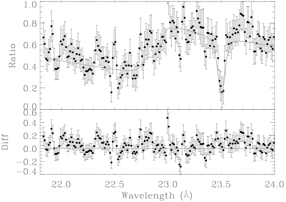
Figure 12: Ratio of the spectra of Figs. 11 and 9 (black data points). This shows the interstellar extinction according to Chandra. Overplotted (grey line) is our interstellar extinction model which includes the 0.13 Å shift of the oxygen edge.

Combining the Chandra spectra of Figs. 11 and 9 yields the interstellar extinction curve according to Chandra, shown in Fig. 12. Since all instrumental features are removed from this plot, it can be directly compared with the corresponding XMM-RGS plot of Fig. 5. The solid grey line in both plots shows our ISM absorption model which is identical in both Fig. 5 and Fig. 12. Although the Chandra profile is much noisier, the profiles are remarkably identical. Even the positive excursions around 22.77 Å which hint at source absorption features, are repeated in the Chandra data although with far less significance. This similarity between the XMM-RGS and Chandra derived interstellar oxygen absorption features confirms the validity of the data analysis.

Table 2: Summary of spectral features around the neutral oxygen-K edge

wavelength		Observed equivalent widtha (mÅ) in source spectrum
(Å)	identification	Mrk421	PKS 2155	3C273	Sco-X1	4U 0614
$23.50\pm 0.01^{\mathrm{b}}$	neutral oxygen 1s-2p interstellar absorption line	$16\pm 3$	$15\pm 3$ $20\pm 5^{\mathrm{d}}$	$20\pm 8$	$60\pm 5$	$70\pm 8$ $80\pm 5^{\mathrm{d}}$
$22.6-23.0^{\mathrm{e}}$	interstellar oxygen-K edge absorption structure	$)^{\rm{f}}$	$)^{\rm{f}}$	$)^{\rm{f}}$	$)^{\rm{f}}$	$)^{\rm{f}}$
$23.05\pm 0.08^{\mathrm{c}}$	instrumental absorption	$)^{\rm{g}}$	$)^{\rm{g}}$	$)^{\rm{g}}$	$)^{\rm{g}}$	$)^{\rm{g}}$
$23.35\pm 0.02$	instrumental absorption	$18\pm 4$	$15\pm 4$ $25\pm 5^{\mathrm{d}}$	$18\pm 6$	$19\pm 4$	$19\pm 3$ $30\pm 7^{\mathrm{d}}$
$22.77\pm 0.03$	possible local intergalactic absorption	$9\pm 2$	$11\pm 6$	<5	<3	<5

• Equivalent width of feature in the RGS spectrum, unless noted otherwise.

• Shifted by $35\pm 10$  mÅ to longer wavelengths with respect to the theoretical position of McLaughin and Kirby, (matrix (1998)).

• Broad structure of Oxygen bound in a solid compound. The error also reflects the broad and asymmetric nature of the feature.

• Equivalent width of feature in the Chandra spectrum.

• The K edge is not sharp, but extends over the indicated range. The edge is shifted by $0.13\pm 0.02$ Åwith respect to the theoretical R-matrix calculations.

• An equivalent width has no meaning for an edge structure.

• Since this instrumental feature is very broad the continuum level and structure is very uncertain. For this reason no equivalent width was determined.

5 Discussion and conclusions

Comparing high resolution X-ray spectra of sources with low and high interstellar extinction, absorption features around the oxygen K edge can be separated into instrumental and interstellar components. A summary of all features identified is presented in Table 2.

A clear signature of the RGS instrumental profile is seen through absorption structures at 23.05 and 23.35 Å. These can be interpreted as the 1s-2p line, broadened and shifted due to the bound state of oxygen on the instrument. A total column depth of oxygen on the RGS instrument of $N_{\rm{O}}=2\times 10^{17}\leavevmode\nobreak\ \rm{cm}^{-2}$ is derived.

The RGS instrumental oxygen edge is remarkably stable over time. Early and later observations of Mrk~421 (orbits 84 and 259) show, within statistical errors, exactly the same structure and magnitude of the edge.

The 23.35 Å feature is also seen in the Chandra LETG spectra. If the 23.05 and 23.35 Å features point to different components, it is clear that the 23.35 Å component is common in both instruments, while the 23.05 Å  component is less prominent in Chandra LETG/HRC.

Likely compounds in the instruments which contain oxygen (apart from the known oxygen in the Chandra filter polyamide carrier) are water(ice) and oxidised metal surfaces.

Both XMM-RGS and Chandra LETG have metal surfaces, which will be slightly oxidised. One could therefore argue that the 23.35 Å feature corresponds to metal oxides. For RGS, the active Si of the RGS CCD detectors is covered with a 270 Å  $\mathrm{MgF_{2}}$ insulation layer which, on top of that, holds an Al light shield, with a thickness in between 450 and 740 Å, depending on the CCD (Den Herder et al. herder (2001)). In the Chandra HRC there is a separate filter which holds an aluminium layer. In both instruments the oxides can be resident on the aluminium filters or optical components. For RGS the computed oxygen column density for the 23.35 Å feature corresponds to an aluminium oxide layer of about 35 Å. An independent measurement, using ellipsometry, of the oxide layer on the top of the Al light shield on one of the flight spare RGS CCDs indicated a layer of only $\approx 10$ Å. Additional metal oxides will be present on the active Si as well on the optics. In the Chandra data the fit of the 23.35 Å feature yields an equivalent aluminium oxide layer thickness of about 110 Å.

The 23.05 Å feature dominates the RGS instrument response. Contamination (ice forming on the cooled detectors) is very unlikely the origin of this absorption feature in view of the stable response of the instrument over a prolonged period of time during repeated observations of Mrk~421. In addition, the relative intensities of the RGS aluminium and fluor calibration sources, which show X-ray lines at 1.487 and 0.677 keV respectively, did not change from before launch to recent times (orbit 440). These intensity ratios are very sensitive to accumulation of oxygen (water-ice) on the detectors.

Another source of oxygen may be absorption of water by the $\mathrm{MgF_{2}}$ insulation layer during manufacturing of the CCD’s, before the Al light shield was applied. This process would lock the water behind the Al light shield, without any possibility to escape. $\mathrm{MgF_{2}}$ is known to be porous, and may be able to absorb considerable quantities of water, depending on the way it was deposited on the CCD surface. When all of the oxygen of the 23.05 Å feature would be in the form of water, we would need a layer of 550 Å to be able to account for the observed column density. Despite the fact that the thickness of the $\mathrm{MgF_{2}}$ layer is only known for the “solid equivalent” (assuming that the $\mathrm{MgF_{2}}$ is not porous), the required quantity of water seems quite large and is hard to account for solely in the 270 Å $\mathrm{MgF_{2}}$.

Laboratory measurements of RGS flight-spare CCDs are consistent with the instrumental oxygen edge measured in flight. The systematic error for the laboratory measurements, however, is high compared to the flight measurement.

The interstellar (ISM) extinction derived from XMM-RGS and Chandra LETG/HRC data is fully consistent between the instruments, confirming the validity of the analysis.

The interstellar component is compared with theoretical predictions based on the R-matrix (McLaughlin and Kirby, matrix (1998)) computations of cross sections for atomic oxygen. There is indication that the theoretical 1s-2p line position requires a slight shift of about $35\pm 10$ mÅ to larger wavelengths. The structure around the K edge is shifted relative to the 1s-2p line by $0.13\pm 0.02$ Å to longer wavelengths (closer to the 1s-2p line), when compared to the theory. The overall shape of the edge, which reflects the detailed resonance structure convolved with the instrument response, fits the actual data well. The total interstellar X-ray absorption fits the expected profile for neutral atomic oxygen. No unambiguous additional signature of oxygen bound in other compounds (e.g. interstellar dust grains) is found. However, we are only sensitive to sufficiently narrow features. If the type of solid state oxygen in dust grains would exhibit very broad absorption features we would not recognise it. An upper limit of oxygen compounds other than neutral oxygen, which have distinct and narrow features around the oxygen edge is estimated at less than 10 % of the neutral oxygen.

A possible interstellar absorption feature of the local intergalactic medium was found around 22.77 Å in both PKS~2155-304 and Mrk~421 spectra. The exact compound causing this possible absorption feature is not unambiguous, but the fact that this feature is not seen in our galactic sources does point to an extragalactic origin. We tentatively identify this feature with O iv absorption.

- (1) Bradshaw, C.F., Fomalont, E.B.,& Geldzahler, B.J., 1999, ApJ, 512 L121
- (2) Brandt, S., Castro-Tirado, A.J., Lund, N., et al. 1992, A&A, 262, L15-L16
- (3) Brinkman, A.C., Gunsing C.J.T., Kaastra, J.S., et al. 2000, ApJ, 530, L111-L114
- (4) Dame, T.M., Ungerechts, H., Cohen, R.S., et al. 1987, ApJ, 322, 706
- (5) Hartmann, D.,& Burton, W.B., 1997, Atlas of Galactic Neutral Hydrogen, Cambridge University Press, ISBN 0-521-47111-7
- (6) Henke, B.L., Lee, P., Tanaka, T.J., et al. 1982, Atomic Data Nucl. Data Tables, 27, 1
- (7) Den Herder, J.W., Brinkman, A.C., Kahn, S., et al. 2001, A&A, 365, L7-L17
- (8) Jansen, F., Lumb, D., Altieri, B., et al., 2001, A&A, 365, L1-L6
- (9) Kaastra, J.S., 2002, Calibration XMM/Chandra using PKS2155-304, SRON internal report.
- (10) Kaastra, J.S., Steenbrugge, K.C., Raassen, A.J.J., et al., 2002b, A&A, 386, 427
- (11) Kaastra, J.S., Mewe, R.,& Raassen, A.J.J., 2002c, Proceedings Symposium ”New Visions of the X-ray Universe in the XMM and Chandra Era”
- (12) Lockman, F.J.,& Savage, B.D., 1995, ApJS, 97, 1
- (13) McLaughlin, B. M., & Kirby, K. P. 1998, J. Phys., 31, 4991
- (14) Menzel A., Benzaid S,. Krause M., et al., 1996, Phys. Rev. A 54, 991
- (15) Morrison, R.,& McCammon, D., 1983, ApJ, 270, 119
- (16) Nicastro, F., Zesas, A., Drake, J., et al. 2002, ApJ, 573, 157
- (17) Paerels, F., Brinkman, A.C., van der Meer, R.L.J., et al. 2000, ApJ, 546, 338
- (18) Sevier, K.D., 1979, Atom. Data and Nuc. Data Tab. 24, 323
- (19) Stolte W.C., Samson, J.A.R., Hemmers, O., et al., 1997, J. Phys. B, 30, 4489
- (20) Wilms, J., Allen, A.,& McCray R., 2000, ApJ, 542, 914