Detailed Analysis of Nearby Bulgelike Dwarf Stars III. $\alpha$ and Heavy-element abundances

Abstract

The present sample of nearby bulgelike dwarf stars has kinematics and metallicities characteristic of a probable inner disk or bulge origin. Ages derived by using isochrones give 10-11 Gyr for these stars and metallicities are in the range -0.80$\leq$ [Fe/H]$\leq$ +0.40. We calculate stellar parameters from spectroscopic data, and chemical abundances of Mg, Si, Ca, Ti, La, Ba, Y, Zr and Eu are derived by using spectrum synthesis.

We found that [$\alpha$-elements/Fe] show different patterns depending on the element. Si, Ca and Ti-to-iron ratios decline smoothly for increasing metallicities, and follow essentially the disk pattern. O and Mg, products of massive supernovae, and also the $r$-process element Eu, are overabundant relative to disk stars, showing a steeper decline for metallicities [Fe/H] $>$ -0.3 dex. [$s$-elements/Fe] roughly track the solar values with no apparent trend with metallicity for [Fe/H] $<$ 0, showing subsolar values for the metal rich stars. Both kinematical and chemical properties of the bulgelike stars indicate a distinct identity of this population when compared to disk stars.

1 Introduction

The inner stellar populations of the Milky Way are a fundamental key for the understanding of the chemical and dynamical history of the Galaxy, and they are templates for the study of unresolved populations in external galaxies. These stellar populations have not been well studied because of the reddening and dust contamination in the line of sight towards the Galactic center. Due to the distance and reddening, basically only luminous objects such as AGB stars, M and K giants and planetary nebulae have been studied in this region, many of them located in windows of low extinction as the Baade’s Window (BW) and the fields of Blanco & Terndrup (1989).

The innermost part of the Galaxy comprises a nucleus, within a few hundred parsecs to the center and the bulge, a structure of about 2.8$\times$2.1 kpc at wavelength of 12$\mu$m according to Habing et al. (1985), or a region within a Galactocentric radius R_GC $<$ 4 kpc if the characteristics of globular clusters are considered (Barbuy et al. 1999a). The nucleus of the Galaxy or the Galactic Center, has a huge molecular cloud, the Central Molecular Zone (e.g. Serabyn & Morris 1996; Lis et al. 2001), with intense star formation, and possibly harboring a black hole (Eckart et al. 2001; Ghez et al. 2000). The bulge is a more extended and sparse component than the Galactic center, with high velocity dispersion, $\sigma$ $\sim$ 100 kms^-1 (e.g. Sadler et al. 1996), and sustained by rotation (e.g. Wyse & Gilmore 1992). Studies of the COBE - DIRBE data and other sources showed that the Milky Way contains a central bar (e.g. Blitz & Spergel 1991; Weiland et al. 1994; Wada et al. 1994; Nikolaev & Weinberg 1997), although it is not clear if bulge and bar are the same structure or share the same stellar populations (e.g. Kuijken 1996; Combes 1998; Gerhard 2000; van Loon et al. 2003 and references therein). The outer border of the bulge, where it connects to the inner disk, and the inner disk itself, still have a poorly known structure (Wyse et al. 1997; Gerhard 2000).

As the center of the gravitation potential well, the inner Galaxy is populated with stars in transit, born in halo and disk environments. Within the Galactic Center, M supergiants, OH-IR, luminous AGB and Wolf-Rayet stars were identified (e.g. Catchpole et al. 1990; Krabbe et al. 1995; Blum et al. 1996; Frogel et al. 1999). Only recently high-resolution metallicities have been reported for some of these objects (Ramirez et al. 2000; Carr et al. 2000), indicating a mean metallicity near the solar one. Age measurements suggest that a fraction of stars of the Galactic center was formed in the last 3-7 Gyr (Tamblyn & Rieke 1993; Krabbe et al. 1995; Frogel et al. 1999).

A few studies of the bulge population have been published during the last two decades (e.g. Whitford & Rich 1983; Rich 1988; McWilliam 1997; Wyse et al. 1997; Wyse 2000; and references therein). Age determinations from HST data have confirmed that most of the bulge stars are old, with $\sim$ 13 Gyr (Ortolani et al. 1995; Feltzing & Gilmore 2000; Ortolani et al. 2001). The metallicity distribution of this population ranges from [Fe/H] $\simeq$ -1.6 to + 0.55 dex (McWilliam & Rich 1994, hereafter MR94) with a mean of [Fe/H] $\approx$ -0.25 or [M/H] $\approx$ 0 (MR94; Zoccali et al. 2003). MR94 and Rich & McWilliam (2000, hereafter RM00) performed a detailed abundance analysis of a sample of K giants in the BW. Abundances of $\alpha$, $r$ and $s$-process elements were derived revealing some peculiarities, with $\alpha$-elements showing different behaviors depending on the element: O, Mg and Ti are overabundant, while Si and Ca show a trend similar to disk stars. $s$-process elements track roughly the behavior of disk stars while the $r$-process element Eu is enhanced.

Very few data were published about inner disk stars and the metallicity distribution of this region has not been investigated in detail. One high-resolution abundance analysis was performed for a sample of B stars showing enhanced chemical abundances relative to solar neighborhood for $\alpha$-elements, except for oxygen (Smartt et al. 2001).

In the present work we derive chemical abundances for a sample of 35 stars pertaining to a population with peculiar kinematics. It consists of stars with highly eccentric orbits, pericentric distances R_p $<$ 5.5 kpc, and absolute vertical velocities of less than 20 kms^-1. Isochronal ages of 10-11 Gyr were inferred for this population (Grenon 1998). The metallicity distribution is identical to that of the bulge sample studied by MR94 (Grenon 1999). The details on kinematical properties and theories about the origin of such population are described in Pompéia, Barbuy & Grenon (2002a, hereafter Paper I) and in a series of papers by Grenon (1990, 1999, 2000), and Castro et al. (1997). The main goal of this work is to analyse a larger sample of these stars in order to improve our knowledge on the chemical distribution of stars from the inner Galaxy. These results could shed some light on the following questions: (1) what is the abundance pattern of this group?; (2) are the chemical distributions of this population similar to the population of any other component of the Galaxy?; (3) given the chemical distributions, what can be inferred about the origin of this population?

2 Observations

Sample stars were observed at the 1.52m ESO telescope at La Silla, Chile, in September 1999. The spectra were obtained using the FEROS spectrograph, with coverage from 356 to 920 nm and resolution of R 48,000. Most spectra have signal to noise ratios S/N $>$ 100. Reductions were performed using the DRS (online data reduction system of FEROS) and for a subsequent reduction, tasks of the IRAF package were applied (see also Paper I).

3 Analysis

3.1 Stellar Parameters

In Paper I, gravities and metallicities were derived enforcing the ionization equilibrium of Fe I and Fe II lines, but the reliability of such method has been questioned. In the atmosphere of late-type stars, Fe I lines are formed under non-LTE (NLTE) conditions, and two main points have been observed about the derived stellar parameters: gravities measured through ionization equilibrium are usually lower than those derived from accurate astrometric values (e.g. Fuhrmann et al. 1997; Nissen et al. 1997; Allende Prieto et al. 1999), and metallicities calculated applying NLTE corrections are higher than those derived by the ionization imbalance (Thevénin & Idiart 1999). In order to increase the accuracy of our abundances, we have reanalyzed the stellar parameters as follows.

As in Paper I, the effective temperatures were estimated by fitting the H$\alpha$ line profiles; trigonometric gravities derived using Hipparcos paralaxes (see Paper I) are adopted; microturbulence velocities were inferred requiring that the $\epsilon$(Fe I) vs. EW (equivalent widths) gives no slope; metallicities were calculated from the Fe II lines and checked with metallicities derived from Geneva photometry. MARCS model atmospheres (Gustafsson et al. 1975) were employed.

The reliability of the determination of temperature of cool dwarf stars by Balmer line profiles has been discussed in detail in literature (e.g. Furhmann et al. 1993, 1994; Furhmann 1998; Cowley & Castelli 2002), even for stars as cool as T_eff $\sim$ 4800 K (Barklem et al. 2002), showing that the involved errors are small.

In Table 1 the inferred stellar parameters are reported. Metallicities derived from both Fe I and Fe II lines are given, together with the standard deviations. Fe I and Fe II line lists and EW are given in Paper I. We have improved our Fe II line list with 5 lines, 6149.25, 6179.40, 7222.39, 7224.46 and 7449.33 $\rm\AA$ from Chen et al. (2003). As expected, metallicities derived from Fe I give smaller values than those derived from Fe II (e.g. Thevénin & Idiart 1999). HD 11306 show a large difference between metallicity values and a high standard deviation for Fe II lines. For this star we chose [FeI/H] = -0.63 which yields the best fit to the stellar spectrum. The uncertainties of the fundamental parameters are: $\sigma$(T_eff) = 50 K; $\sigma$(log $g$) = 0.15 dex, $\sigma$([Fe/H]) = 0.10 dex; and $\sigma$ $\xi_{t}$ = 0.10.

3.2 Line List

Atomic lines are selected based on the paper of MR94, and improved with lines of Barbuy et al. (1999b, 2003) and Smith et al. (2000). Oscillator strengths, adopted from the cited papers and other sources (see Table 2), are tested by fitting the synthetic to the observed line profiles in the Solar Flux Atlas of Kurucz et al. (1984). The solar abundances are from Grevesse et al. (1996). Synthetic lines with a very good match to the solar spectra are chosen, with the exception of one barium line, which is discussed below. In Table 2 we give the atomic line list for the $\alpha$ and heavy-element lines used in this work.

Oxygen abundances derived in Paper I are recalculated using the new stellar parameters and taking into account the Ni I line at 6300.34 $\rm\AA$ with log gf = -2.31 (Allende Prieto et al. 2002). For the solar abundance we adopted [O/Fe] = 8.77. Hyperfine structures (HFS) for the Eu I 6645.41 $\rm\AA$ and the Ba II 4554.03, 4934.10 and 6496.41 $\rm\AA$ lines are taken into account following François (1996 and private communication) and Hill et al. (2000). Below we discuss the selected line list.

3.2.1 $\alpha$-elements

The four selected Ca I lines are relatively intense and were well fitted to the solar spectrum. Six Ti I lines were chosen, with three moderately weak lines at 6303.77, 6312.24 and 6336.11 $\rm\AA$. Such lines are near to the Fe I features at 6303.46 and 6336.83 $\rm\AA$, but we found a good separation between lines thanks to the high resolution and good quality of the spectra. The Ti I line at 6554.22 $\rm\AA$ is also near the H$\alpha$ profile, which required a careful definition of the continuum near lines.

Three of the five Si I lines adopted, at 6237.33, 7405.79 and 7415.96 $\rm\AA$, are moderately intense. Although the two last features are blended to CN and Cr I lines, the spectrum synthesis yielded a good match to the solar spectrum. The remaining two Si I 6721.84, and 7226.21 $\rm\AA$ lines are weak but apparently free of blendings. Only the line 6319.24 $\rm\AA$ from the magnesium triplet at 6316 - 6319 $\rm\AA$ showed a good fit to the solar spectrum. The second Mg I line adopted, at 7387.70 $\rm\AA$, has features of Co I near the blue wing, and Mg I in the red, but we found a good agreement between solar and synthetic features.

3.2.2 Heavy elements

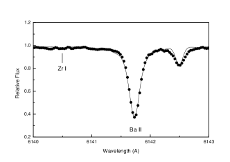
Figure 1: Synthetic fit in the region of the Zr I 6140.46 $\rm\AA$ and Ba II 6141.73 $\rm\AA$ lines for the star HD 152391.

Both La II lines are very small features even if free of blendings. Therefore most of the derived abundances for this element represent upper limits. Also the adopted zirconium Zr II 6114.85 $\rm\AA$, and Zr I 6134.57, 6140.46 and 6762.40 $\rm\AA$ lines are very small. The line at 6140.46 $\rm\AA$ is near the strong Ba II feature at 6141.73 $\rm\AA$, which required a more careful fit of the continuum. In Figure 1 we show the synthetic and observed spectra of this region for HD 152391. Yttrium and europium are represented in our sample by the single weak lines Y I 6795.41 and Eu II 6645.10 $\rm\AA$ respectively. The Y I line is near the Fe I 6795.80 $\rm\AA$ feature, but no blendings were observed. Y, Zr and La show very small features in the spectra of the stars (see Tables 4 and 5), and hyperfine structures were not taken into account in the abundance analysis.

Barium, a special case: barium lines are very intense and with many isotopic components, some subject to hyperfine splittings. Although many isotopes are present in the resonant lines, the isotopic shifts are very small, $\leq$ 2 m$\rm\AA$ (Mashonkina et al. 1999). Three Ba II lines are adopted to infer the barium abundances: the resonance lines at 4554.03 and 4934.10 $\rm\AA$, and one line in the red, 6496.91 $\rm\AA$. Atomic HFS components of François (1996 and private communication), based on the HFS of Rutten (1978), are adopted.

In the synthesis of the solar spectrum, where the barium lines are saturated, we found a non-solar barium abundance, [Ba/Fe] = +0.22, for the 6496.91 $\rm\AA$ line (see sect. 3.3.2). We also found that the core of the observed profile of this line and the two resonant lines are slightly deeper than the synthetic ones. Due to the saturation, the core of these lines form in a shallower atmospheric layer, under NLTE conditions. Problems with abundance analysis of barium lines have long been discussed in the literature (e.g. Rutten 1978; Magain 1995; Sneden et al. 1996; McWilliam 1997; Mashonkina et al. 1999, Mashonkina & Gehren 2000), particularly involving the fitting of the core of the solar Ba II lines, as described by Mashonkina et al. (1999) and Mashonkina & Gehren (2000), and non-solar abundances have been reported for the synthesis of these lines (e.g. Smith et al. 2000).

3.3 Abundances

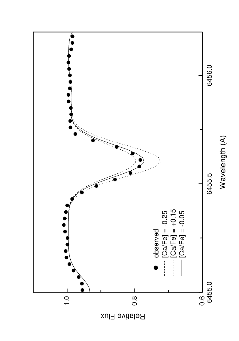
Figure 2: Examples of the fitting procedure for HD 10758. Observed (dots) and synthetic (lines) spectra for three abundance values (see the legends) around Ca I 6455.60 $\rm\AA$ and Ba II 6496.91 $\rm\AA$ lines. The best fit give [Ca/Fe] = 0.05 and [Ba/Fe] = 0.25.

LTE stellar abundances of Mg, Si, Ca, Ti, Y, Zr, Ba, La and Eu are derived by fitting the synthetic to the observed spectra. The spectrum synthesis code is described in Cayrel et al. (1991) and Barbuy et al. (2003). The synthetic spectra were convolved with Gaussian profiles with FWHM from 0.10 to 0.15 $\rm\AA$. Molecules of MgH (A${}^{2}\Sigma-\rm X^{2}\Pi$), C${}_{2}(\rm A^{3}\Pi-\rm X^{3}\Pi)$, CN blue ($\rm B^{2}\Sigma-\rm X^{2}\Sigma$), CH ($\rm A^{2}\Delta-\rm X^{2}\Pi$), CH ($\rm B^{2}\Delta-\rm X^{2}\Pi$), CN red ($\rm A^{2}\Pi-\rm X^{2}\ Sigma$) and TiO $\gamma$ ($\rm A^{3}\Phi-X^{3}\Delta$) are included. In Figure 2 we show the fit to the Ca I 6455.60 $\rm\AA$ line (top) and the Ba II 6496.91 $\rm\AA$ line (bottom) for HD 10758. In Table 3 we report the derived abundances along with the scatter (standard deviation) among different lines. In Tables 4 and 5, equivalent widths are given for each line.

3.3.1 Continuum absorption for $\alpha$-enhanced atmospheres

The continuum absorption has been computed by taking into account the $\alpha$-element (O, Mg, Si, Ca and Ti) enhancement for the stars showing [$\alpha$/Fe] $\geq$ 0.2, as being equal to 0.2. This is important because the $\alpha$-elements are electron donors (magnesium being the most important element in this respect). With $\alpha$ enhancement the electron pressure increases, therefore the continuum absorption by H^- increases. As a consequence, a certain optical depth will be reached at a shallower layer, where the gas pressure is lower, therefore the line wings will be less strong.

The continuum is affected in two ways: (i) molecular bands or a number of atomic lines involving the $\alpha$-elements will affect indices in the pseudo-continuum as well as the features; (ii) the true continuum is dominated by H^-, and therefore it will depend on electron donors, among which the $\alpha$-elements Mg and Si are important, whereas Ti is not important in this respect.

3.3.2 Abundance Errors

Errors in derived abundances depend on many factors. The uncertainties in stellar parameters are an important error source. To evaluate the effect of these uncertainties, we changed the stellar parameters of HD 143016 and HD 10576 by $\Delta$ T_eff +50 K, $\Delta$ log $g$ = +0.15 dex, $\Delta\xi$ = +0.10 and [Fe/H] = 0.10 dex, and calculated the abundance variations. Abundance changes are summarized in Table 6, where the total errors, $\delta_{t}$, are also given. Table 6 also shows that most abundances vary by less than 0.1 dex, with a maximum value of 0.15 dex.

The scatter among different lines given in Table 3 are probably due to a sum of factors: uncertainties in the adopted oscillator strengths and stellar parameters, and due to NLTE and blending effects. Abundances estimated by using very weak lines as Zr I lines, are subject to errors due to the adoption of upper limits.

Some of the lines studied here form under departure from LTE, therefore, errors due to non-LTE (NLTE) conditions should be considered. Zhao et al. (1998) studied NLTE effects on the abundances derived from Mg I lines. They found a difference of 0.05 dex between NLTE and LTE analysis for the Mg I 6319.49 $\rm\AA$ line. NLTE effects for Mg I lines were also derived for a large sample of dwarf stars by Shimanskaya & Mashonkina (2001), where it was found that standard errors for most of the stars are $\leq$ 0.07 dex. Ca I lines are subject to NLTE effects, however Drake (1991) found that the errors are negligible for dwarf stars. Thorén & Feltzing (2000) and Thorén (2000) found small changes between LTE and NLTE abundances for Ca I lines in cool dwarf stars, with T_eff $\leq$ 5800 K.

NLTE effects as high as $\sim$0.2 dex were inferred by Mashonkina & Gehren (2000) for the Ba II 6496.91 $\rm\AA$ line in some cool dwarf stars. In spite of such a high discrepancy, we found a satisfactory agreement among lines for our sample stars, and all Ba II lines are taken into account in the abundance analysis. Another error source for the barium lines is the $r$/$s$ solar mixture choice (Sneden et al. 1996). It affects the isotopic splittings since odd-isotopes are mainly produced by the $r$-process, while even isotopes, by the $s$-process. But changes of $\sim$ 0.1 dex or less are expected in abundances due to different isotopic distributions (Burris et al. 2000).

4 Results

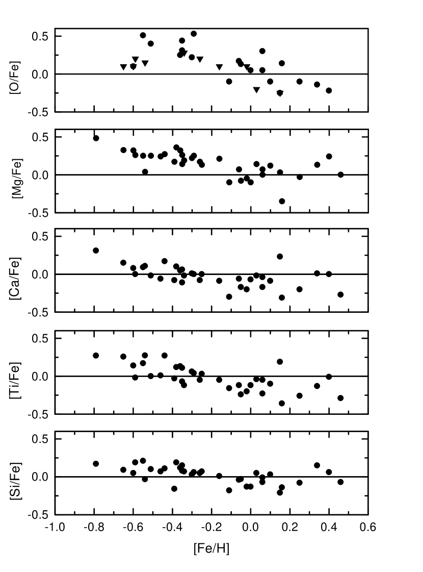
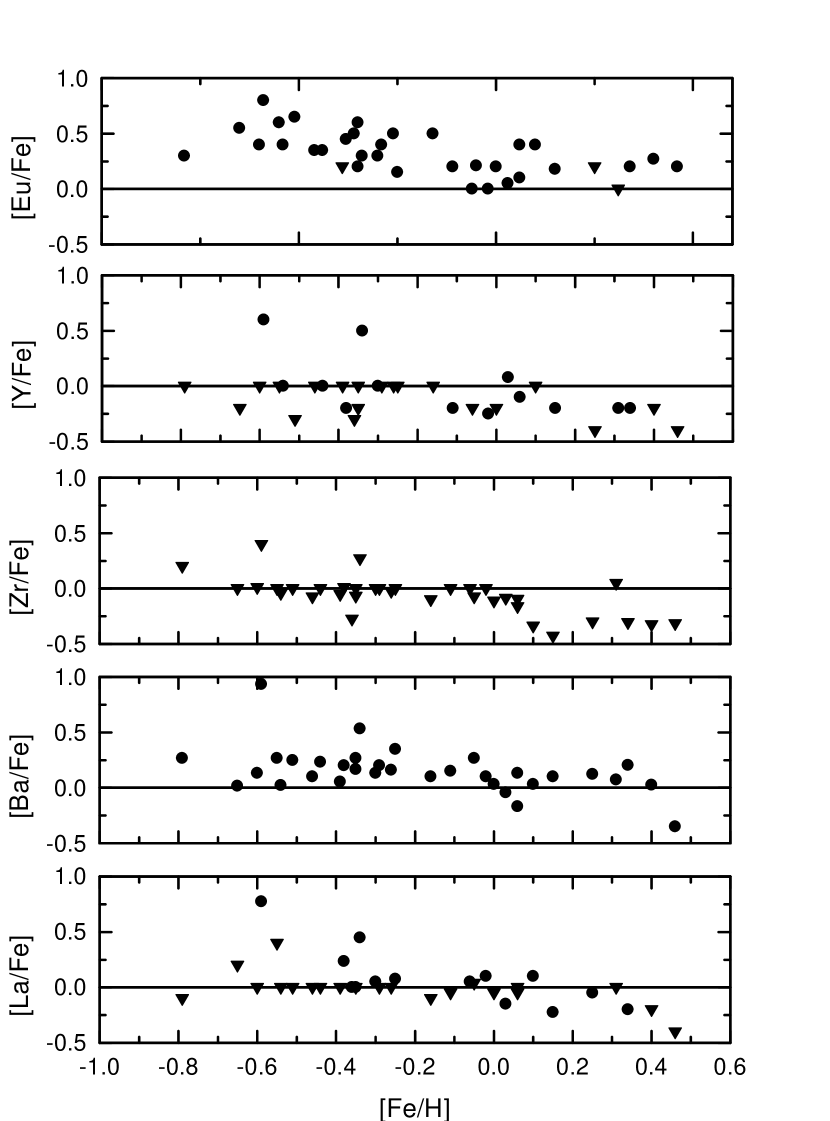
Figure 3: [$\alpha$/Fe] (left), [$r$-process/Fe] and [$s$-process/Fe] (right) vs. [Fe/H] relations for the bulgelike stars. Downtriangles represent upper limits.

In Figure 3 we show the abundance trends for the sample bulgelike stars. Upper limits are depicted by down triangles. It seems from these plots that the $\alpha$-elements have different behaviors depending on the element, and can be roughly divided into two groups. The first group includes Si, Ca and Ti, and the second, O and Mg, which have similar pattern (except for the upper limit values) to the $r$-process element Eu. In the following sections we describe the derived distributions and the formation theories of these elements.

4.1 Si, Ca and Ti

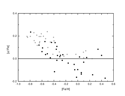
Figure 6: [$\alpha$’/Fe] vs. [Fe/H] relation: $\bullet$ present sample, + Edv93.

Si and Ca are prototypical $\alpha$-elements, synthesized during hydrostatic burning of massive stars (Woosley & Weaver 1995), with a small contribution by Type Ia supernovae (SN Ia) (Tsujimoto et al. 1995). The typical enrichment timescale of the interestellar medium (ISM) due to massive stars is of some $\sim$ 10⁶ yr. The formation efficiency of both Si and Ca depends on the mass of the progenitor of the Type II supernova (SNe II). The production factor of these elements are larger for a $\approx$ 25 M_⊙ progenitor, while declining factors are predicted for lower or higher mass stars (see Figure 6 of RM00). Nucleosynthetic prescriptions associate Ti formation to the iron peak elements (Thielemann et al. 1996), but the observations strongly suggest connections with the $\alpha$-elements (e.g. Wheeler et al. 1989; Edvardsson et al. 1993, hereafter Edv93; Chen et al. 2000, hereafter Chen00).

In Figure 3, the [$\alpha$-elements/Fe] vs. [Fe/H] distributions for Si, Ca and Ti are depicted. Such elements show a monotonic decrease with increasing metallicity for metallicities [Fe/H] $<$ -0.2. In the metallicity range -0.2 $<$ [Fe/H] $<$ +0.2, a change in the declining trend, with a flatter pattern and many subsolar values, is seen. An interesting result from our analysis is the notorious similarity between Ca and Ti abundances, with a correlation coefficient of $r$ = 0.89, possibly indicating a common nucleosynthetic process.

4.2 O, Mg and Eu

O and Mg are produced in massive SNe II ($\sim$ 35 M_⊙), and these elements are not predicted in the yields from intermediate to low mass stars (Woosley & Weaver 1995; Thielemann et al. 1996). Eu is produced by the $r$-process through rapid neutron captures onto seed nuclei (e.g. Thielemann et al. 1990). The astrophysical site for this process is still debated (Wallerstein et al. 1995; Hoffman et al. 1997; Thielemann et al. 2001) and some possible sites have been suggested: SN II explosion (e.g. Woosley & Hoffman 1992; Takahashi et al. 1994), neutron stars merging (Davies et al. 1994; Rosswog et al. 1999, 2000) and the coalescence of a neutron star and a black hole (Thielemann et al. 2001).

O, Mg and Eu abundances relative to iron in our sample show a slower decrease with increasing metallicity for -0.8 $\leq$ [Fe/H] $\leq$ -0.2, when compared to Ca, Ti and Si. Beyond this value, a decline is seen followed by an almost constant trend in the range -0.2 $<$ [Fe/H] $<$ + 0.2, with Mg showing few subsolar values. For metallicities above the solar value, Mg and Eu seem to increase with increasing [Fe/H]. [Eu/Fe] show a high scatter for all the metallicity range of the sample.

4.3 $s$-process elements

[$s$-element/Fe] vs. [Fe/H] distributions are also plotted in Figure 3. The $s$-process nucleosynthesis consists of slow neutron captures, which occur in intermediate to low mass AGB stars (e.g. Käppeler et al. 1989). The efficiency of such process basically depends on: (i) the abundance of the iron-peak elements, which are the seed nuclei for the $s$-process; (ii) the neutron density at the $s$-process site; (iii) the ¹³C available below the convective envelope at the so called ”¹³C pocket” - note that the ¹³C($\alpha$,n)¹⁶O is the main source of neutrons in low mass AGB stars (see Gay & Lambert 2000); and (iv) the abundance of the neutron poisons, i.e., elements with high cross sections for neutron capture (Gallino et al. 1998; Busso et al. 2001). As these factors behave diversely with metallicity, a complex run of the [$s$-element/Fe] ratios with metallicity is expected (Busso et al. 1999, 2001).

In our sample, the [$s$-element/Fe] values roughly track the solar one, with apparently no trend with metallicity. Ba shows overabundant values for almost all stars. Y, in opposite way, show many subsolar values. La and Zr nearly follow the solar abundance with a possible trend of decrease for higher metallicities. Two stars seem detached from the others in these plots: HD 11397 and HD 14282. HD 11397 has strong $s$-process lines, and was identified as a CH star by Šleivyte & Bartkevičius (1990). It has also a high Li abundance compared to other bulgelike stars (Pompéia et al. 2002b, Paper II) as expected for stars belonging to binary systems. HD 14282 is moderately enriched in $s$-process elements and has lower Li abundance.

5 Comparison to other samples

In this section we compare the chemical distributions of our sample to previous work on the same kinematical sample (Barbuy & Grenon 1990, hereafter BG90; Castro et al. 1997, hereafter Cas97); to disk samples of Edv93, Nissen & Edvardsson (1992, hereafter NE92), Chen00, Carretta et al. (2000, hereafter CGS00), Feltzing & Gustafsson (1998, hereafter FG98), Thorén & Feltzing (2000, hereafter TF00), Smith et al. (2001, hereafter SCK01) and Koch & Edvardsson (2002, hereafter KE02); as well as to bulge samples of MR94 and RM00, and results for the bulge globular cluster NGC 6553 by both Barbuy et al. (1999b) and Cohen et al. (1999). As discussed before (e.g. Prochaska et al. 2000), the temperature scale of Edv93 has an offset of $\Delta$T_eff $\sim$ +100 K when compared to temperatures derived by using the Infrared Flux Method (IRFM) and from H$\alpha$ profiles (Gratton et al. 1996). As our temperatures are inferred from H$\alpha$ profiles, and they agree with IRFM temperatures (Paper I), we modified the Edv93 data by applying the corrections given in their Table 6, for a temperature change of $\Delta$T_eff = -100 K.

5.1 Comparison with BG90 and Cas97

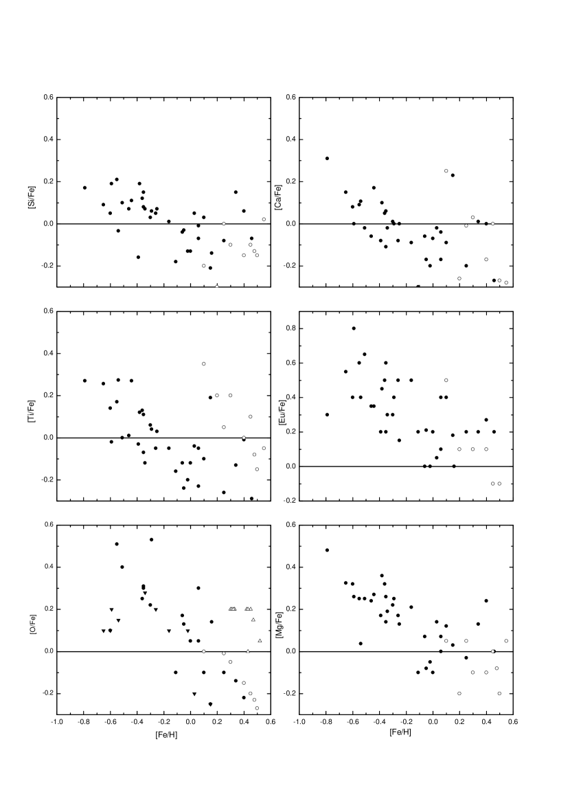
Figure 4: [X/Fe] vs. [Fe/H] relations: $\bullet$ present sample compared with $\circ$ Cas97 and $\triangle$ BG90 samples.

Metal-rich stars ([Fe/H] $\geq$ + 0.2 dex) from the same kinematical sample of our stars have been studied by BG90 and Cas97. BG90 derived oxygen abundances from the [O I] line at 6300 $\rm\AA$ for a sample of 11 stars. Cas97 also derived oxygen abundances from this line, and abundances of Mg, Si, Ca, Ti and Eu among others, for a sample of 9 stars. In Figure 4 we compare our data to BG90 and Cas97. BG90 found an almost continuous value of [O/Fe] $\approx$ + 0.2 for their sample stars and Cas97 found a steep decline in oxygen to iron ratios for increasing metallicities. Our results are similar to Cas97, although showing a higher scatter. For Mg, Si and Ca, Cas97 values appear as a natural sequence of our decreasing trends to higher metallicities. For Ti, a steeper decline with metallicity is observed in Cas97 compared to our abundance ratios. Our Ti determinations are based on six lines, a higher number of lines than that adopted by Cas97, and the trend from our data should be reliable. The overabundant behavior of our [Eu/Fe] values appear to be present also for the higher metallicities of the Cas97 sample.

5.2 Si, Ca and Ti

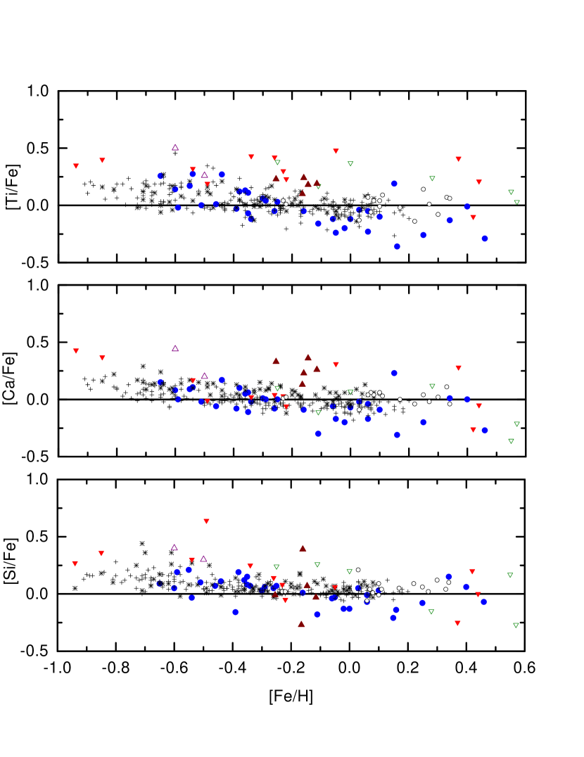
Figure 5: [$\alpha$/Fe] vs. [Fe/H] relations for Ti, Ca and Si: present sample (filled circles), Edv93 (crosses), Chen00 (stars), TF00 (open circles), MR94 (filled downtriangles), and RM00 (open downtriangles), Cohen et al. (1999) (filled triangles), and Barbuy et al. (1999) (open trianlges).

In Figure 5, our sample is compared to disk and bulge results. This figure shows that Si, Ca and Ti follow the disk trend, with a possible steeper decline for increasing metallicities. In Figure 6 we compare the mean of Si and Ca ratios, [$\alpha$’/Fe], to the same ratio of Edv93, for stars with mean galactocentric radius R_m $<$ 7 kpc. We found that the two samples essentially overlap, showing that the abundances of these elements are similar to those of the disk with smaller R_m.

The comparison with the bulge stars shows that our sample show similar values of [Ca/Fe]. On the other hand, the bulge shows higher [Si/Fe] and even higher [Ti/Fe] values, with no apparent declining trend with metallicity. The results from both Barbuy et al. (1999b) and Cohen et al. (1999) for NGC 6553 show higher Si, Ca and Ti abundances, even if the [Fe/H] value found for the cluster differ in these studies ([Fe/H] = -0.55 from Barbuy et al. and [Fe/H] = -0.17 from Cohen et al.).

For metallicities above solar, the samples of Edv93, FG98 and TF00 suggest a roughly constant [Si/Fe] ratio and [Ca/Fe] with a possible decreasing trend. But such trends are not confirmed by Chen00 and Cas97. Our sample, as well as bulge stars from MR94, have a larger scatter with no well-defined trend. For Ti, results from Edv93 show a slightly decreasing pattern, and the opposite behavior is seen in Chen00’s sample.

5.3 O, Mg and Eu

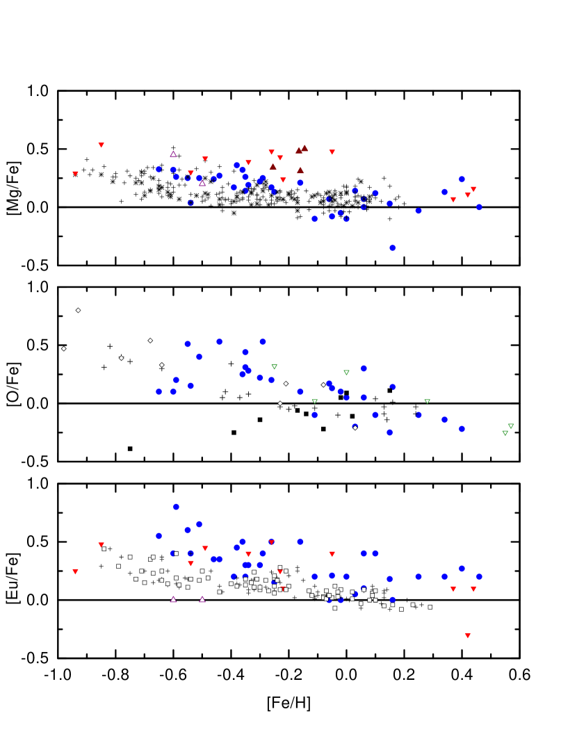
Figure 7: [$\alpha$/Fe] vs. [Fe/H] relations for Mg, O and Eu. Symbols as in Figure 5 except for oxygen, for which we adopted Nissen & Edvardsson (1992) (crosses), and more data from: Carretta et al. (2000) (open diamonds), Smith et al. (2001) (filled squares), and Koch & Edvardsson (2002) (open squares) (see text).

Compared to results for disk stars of NE92, CGS00, SCK01 and KE02, the present sample shows an enhanced pattern for Eu for almost all the metallicity distribution (Figure 7), while Mg and O abundance ratios (when oxygen upper limits are not taken into account) are among the highest values of the disk for [Fe/H] $<$ -0.1. Relative to bulge stars, an overlap is apparent for [Eu/Fe] and [O/Fe], with lower [Mg/Fe] values for the bulgelike stars.

There is a contradictory behavior between O and Mg for supersolar metallicities in NE92, Edv93, FG98 and CGS00 samples. While [Mg/Fe] shows an upturn with increasing trend, [O/Fe] seems to decrease with increasing metallicities. According to GGS00, such behavior suggests that the O/Mg ratio produced in SN II vary as a function of metallicity. The bulge stars seem to follow those trends. Eu observations of disk stars of higher metallicities show conflicting results: while Tomkin et al. (1997) and FG98 found that [Eu/Fe] values increase with metallicity, Woolf et al. (1995), Cas97 and Mashonkina & Gehren (2000) samples point to a decreasing trend. Our data seem to agree with the first group. In the high metallicity range we have very few data and the behavior analysis in this range is not possible.

5.4 $s$-process elements

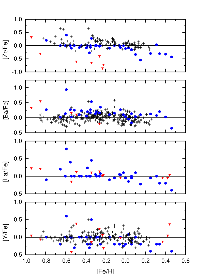
Figure 8: [s-elements/Fe] vs. [Fe/H] relation for Zr, Ba, La and Y. Symbols as in Figure 5.

Fewer data are available in the literature for the s-process elements. In particular, La has very few data in the present metallicity range, and in Figure 8 this element is compared only to the bulge sample of MR94. As can be seen from this Figure, Zr follows the disk distribution with a lower mean value. Compared to bulge stars of MR94, our [Zr/Fe] values are enhanced, although MR94 decided not to use their Zr abundances. Y and Ba distributions for the present sample overlap those of disk stars, with [Ba/Fe] values comparable with the highest values of the disk and apparently following the bulge pattern, while our [Y/Fe] values are comparable with the lowest disk and bulge values. For La a good match between our distribution and the bulge sample is found.

6 Discussion

We draw a series of inferences regarding the sample stars:

1. Abundance trends depend on the star formation history of a given population. In a star forming region, the yields of the SNe II are the first to enrich the interestellar medium (ISM). A large fraction of the iron peak elements is produced later by the SNe Ia, after $\sim$ 1-2 Gyr (e.g. Yoshii et al. 1996). Therefore, in the [$\alpha$/Fe] vs. [Fe/H] plot, a constant [$\alpha$/Fe] ratio or a ”plateau” is seen at low metallicities. When the first SNe Ia begin to explode, this ratio has a downturn, and a knee in the [$\alpha$/Fe] vs. [Fe/H] curve is seen (see e.g. Figure 1 of RM00, McWilliam 1997, Barbuy 1988 and Barbuy & Erdelyi-Mendes 1989).

As well illustrated in Fig. 4 of Matteucci & Brocato (1990, hereafter MB90), for the bulge, the point of downturn of [$\alpha$/Fe] vs. [Fe/H] curves at higher metallicities is a result of a star formation rate more efficient than in the solar vicinity combined to a timescale of formation of the system much shorter (estimated to be of the order 10⁷ yr for the bulge by MB90, but probably somewhat less extreme for the present sample). For the present sample the point of inflexion for [O/Fe], [Mg/Fe] and also that of the $r$-element [Eu/Fe] is around [Fe/H] $\approx$ -0.2, only somewhat less than the estimations for the bulge by MB90. In other words, the knee position in the plot gives information on the star formation rate (SFR). If the SFR is high, a higher metallicity is achieved before the first SNe Ia explode, and the knee is deviated to the right. A fast SF has certainly occurred for our sample stars as well as for the bulge.

2. The level of overabundance of the [$\alpha$/Fe] plateau at low metallicities gives hints on the initial mass function (IMF) of the system. The larger the number of massive stars, the highest the plateau.

3. The slow decreasing trends of Si and Ca with [Fe/H] support the idea that such elements are produced by both SNe II and SNe Ia (Matteucci et al. 1999). Ti follows the same behavior of Si and Ca, also hinting for a production by both SNe types as discussed in previous work (McWilliam 1995a,b). Nevertheless, Ti still has a poorly known formation process and yield predictions (Timmes et al. 1995; Nagataki 1999; Thielemann et al. 2002). Moreover, although in the bulge stars of MR94 and RM00 the other [$\alpha$/Fe]-elements show a similar pattern to our sample, Ti has a puzzling behavior, with an apparently constant value for almost all the present metallicity range.

4. An interesting feature of the $\alpha$-elements distribution in the present sample is the point where the abundance ratios stop the decreasing trend. This occurs for all $\alpha$-elements, with many subsolar values for roughly the same metallicity, [Fe/H] $\sim$ -0.1 dex. Nevertheless, for Ti the subsolar ratios can indicate a systematic error or NLTE effect as discussed by Luck & Bond (1985) and Prochaska et al. (2000). If real, such behavior could be explained by a starburst formation followed by a long interval with negligible SF (Gilmore & Wyse 1991). During this interval the SNe Ia proceed exploding, raising the metallicity of the ISM and eventually decreasing the [$\alpha$/Fe] ratios of the newly forming stars.

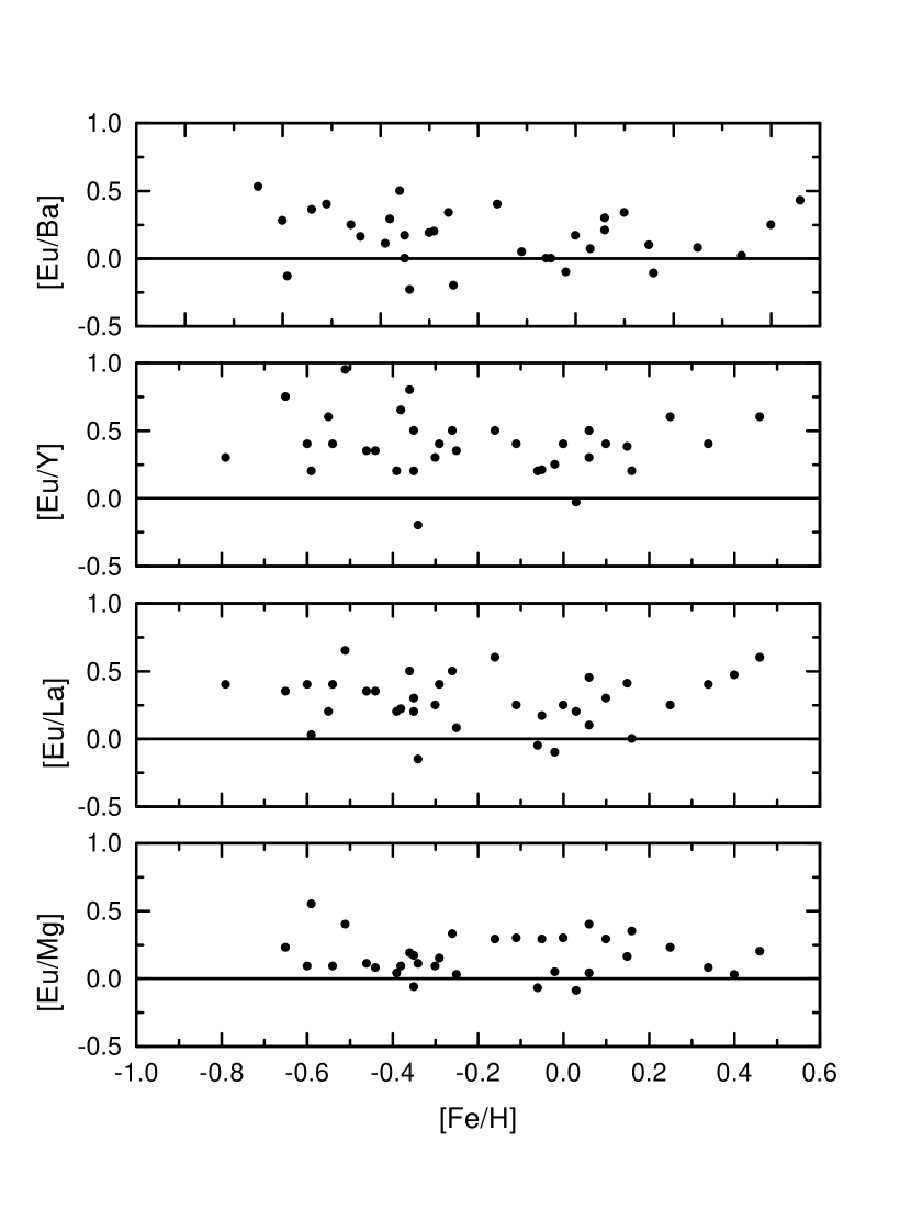
Figure 9: [Eu/X] vs. [Fe/H] relation for the $s$-elements Ba, La and Y, and for the $\alpha$-element Mg.

5. $s$-elements indicate a late evolution of the population given that they are mainly produced by AGB stars in typical timescales of 2-3 Gyr (e.g. Pagel & Tautvaišiene 1997). However a small contribution by the $r$-process is also expected (Truran 1981). A useful diagnostic of the relative importance of the neutron capture processes is the [Eu/$s$] ratio, given that Eu is an almost pure (95%) $r$-process element. In Figure 9 the [Eu/$s$] vs. [Fe/H] relation for Ba, La and Y are plotted, as well as for the $\alpha$-element Mg. [Eu/s-element] curves show a very slow decrease with metallicity until [Fe/H] $\sim$ -0.10, possibly related to the delayed enrichment of the interstellar medium in $s$-elements by AGB stars relative to SNe II. Such decrease is in contrast with the almost constant behavior of [Eu/Mg] over all the metallicity range, suggesting the common origin of these elements. For higher metallicity stars, an increasing trend is seen also hinting for a late burst of SF.

6. The high metallicity of the stars and high eccentricity of the orbits of the present sample points to a probable inner disk or bulge origin. The old and narrow age range of the sample (Grenon 1998) also support this hypothesis. The presence of inner Galaxy stars in the solar neighborhood has been predicted by dynamical simulations of particles under a bar potential well, which triggers chaotic ”hot” movements towards the center and anti-center directions (e.g. Zhao et al. 1994; Raboud et al. 1998; Fux 1997, 2001). From the chemical distribution of our sample, a fast star formation within a possible starburst regime is inferred. If such stars are indeed bulge stars, this result is consistent with an inside-out scenario of Galaxy formation, with a short timescale for bulge formation (MB90; Wyse & Gilmore 1992; Matteucci & Romano 1999, Matteucci et al. 1999). The inner disk origin hypothesis is more difficult to be evaluated because of the paucity of data for the metallicity distribution, age, and chemical features of stars of this region.

7 Summary

In the present work we show that on chemical and kinematical grounds the bulgelike sample represents a distinct population when compared to the disk population. Eu/Fe, O/Fe and Mg/Fe abundance ratios show an enhanced pattern relative to disk stars, a signature of a higher enrichment by SNe II yields, indicating a faster evolution process when compared to the disk.

The point of inflexion of [O, Mg, Eu/Fe] vs. [Fe/H] curves at metallicities [Fe/H] $\approx$ -0.2 are a result of a star formation rate more efficient than in the solar vicinity, combined to a shorter timescale of formation of the system. The point of inflexion derived from our observations is at a somewhat lower metallicity than the estimations for the bulge by MB90.

Si and Ca, on the other hand, follow the disk and bulge trends, consistent with the theories of different sites of nucleosynthetic formation. Ti has a puzzling behavior when compared to bulge stars. In our sample it follows the disk trend while in bulge stars it has an almost constant and high value.

The differences between the $\alpha$-elements O, Mg on one hand, and Si and Ca on the other, has already been found in other samples, in particular the field bulge stars studied by MR94 and RM00, as well as in bulge clusters by Barbuy et al. (1999).

From the chemical distributions of our sample, a fast star formation within a possible starburst regime is inferred. If such stars are indeed bulge stars, this result is consistent with an inside-out scenario of Galaxy formation, with a short timescale for bulge formation (MB90; Wyse & Gilmore 1992; Matteucci & Romano 1999, Matteucci et al. 1999).

$Acknowledgments$ L. P. acknowledges R. Gallino, K. Nomoto, G. Tautvaišiene, T. Tsujimoto, Y. Z. Qian and C. Fryer for very useful discussions during the ”Stellar Abundances and Nucleosynthesis Conference”, and the organizers of this excellent meeting, in particular G. Wallerstein, for this opportunity and financial support. We gratefully thank A. McWilliam and V. Hill for very useful discussions on hyperfine structures. L. P. thanks A. Ardila-Rodriguez and R. R. Rosa for technical support. L. P. acknowledges FAPESP PhD and pos-doc fellowships n^o 98/00014-0 and 01/14594-2. We acknowledge FAPESP project n^o 1998/10138-8.

Table 1: Atmospheric Parameters for the sample stars

Name	Number	Teff	log g	[FeI/H]	$\sigma$(FeI)	[FeII/H]	$\sigma$(FeII)	$\xi(\rm kms^{-1})$
HD 143016	b1	5575	4.11	-0.59	0.12	-0.35	0.14	0.70
HD 143102	b2	5500	3.85	-0.02	0.13	0.03	0.16	1.05
HD 148530	b3	5350	4.43	-0.12	0.14	0.10	0.15	0.80
HD 149256	b4	5350	3.73	0.30	0.16	0.34	0.16	0.80
HD 152391	b5	5300	4.45	-0.12	0.14	-0.05	0.12	0.50
HD 326583	b6	5600	3.81	-0.44	0.13	-0.30	0.17	0.60
HD 175617	b7	5550	4.56	-0.50	0.09	-0.44	0.14	0.60
HD 178737	b8	5575	3.90	-0.37	0.13	-0.35	0.14	0.60
HD 179764	b9	5450	4.26	-0.12	0.13	0.06	0.10	1.10
HD 181234	b10	5350	4.25	0.25	0.14	0.40	0.19	1.10
HD 184846	b11	5600	4.40	-0.29	0.10	0.06	0.07	0.50
BD-176035	b12	4750	4.36	0.21	0.15	0.46	0.13	0.70
HD 198245	b13	5650	4.31	-0.69	0.11	-0.60	0.10	0.60
HD 201237	b14	4950	4.08	0.13	0.16	0.15	0.18	0.50
HD 211276	b15	5500	4.05	-0.61	0.13	-0.39	0.14	0.50
HD 211532	b16	5350	4.46	-0.69	0.15	-0.54	0.18	0.80
HD 211706	b17	5800	4.25	-0.04	0.12	0.16	0.22	0.80
HD 214059	b18	5550	3.81	-0.17	0.11	-0.38	0.14	0.75
CD-40 15036	b19	5350	4.34	-0.11	0.12	0.00	0.13	0.70
HD 219180	b20	5400	4.35	-0.73	0.15	-0.46	0.03	0.65
HD 220536	b21	5850	4.17	-0.23	0.11	-0.11	0.10	0.50
HD 220993	b22	5600	4.15	-0.33	0.12	-0.16	0.08	0.80
HD 224383	b23	5800	4.14	-0.07	0.12	-0.06	0.11	1.00
HD 4308	b24	5600	4.31	-0.45	0.10	-0.26	0.09	0.80
HD 6734	b25	5000	3.40	-0.50	0.09	-0.36	0.10	0.75
HD 8638	b26	5500	4.38	-0.47	0.10	-0.29	0.13	0.60
HD 9424	b27	5350	4.35	-0.03	0.14	0.25	0.12	0.70
HD 10576	b28	5850	4.00	-0.16	0.08	-0.02	0.10	1.25
HD 10785	b29	5850	4.16	-0.25	0.11	-0.25	0.16	1.20
HD 11306	b30	5200	4.09	-0.63	0.11	-0.98	0.19	0.80
HD 11397	b31	5400	4.34	-0.76	0.10	-0.59	0.15	0.65
HD 14282	b32	5800	3.91	-0.43	0.12	-0.34	0.14	0.65
HD 16623	b33	5700	4.26	-0.60	0.09	-0.51	0.15	0.60
BD-02 603	b34	5450	3.75	-0.77	0.12	-0.79	0.14	0.70
HD 21543	b35	5650	4.37	-0.62	0.10	-0.55	0.15	0.50

Table 2: Atomic Line List

Element	$\lambda$	$\xi$exc	log $gf$	Reference
Ca I	6161.30	2.52	$-$1.03	S
Ca I	6455.60	2.52	$-$1.28	B
Ca I	6508.85	2.52	$-$2.50	MR
Ca I	6572.79	0.00	$-$4.30	N
O I	6300.31	0.00	$-$9.76	C
Ti I	6303.77	1.4	$-$1.57	N
Ti I	6312.24	1.46	$-$1.55	N
Ti I	6336.11	1.44	$-$1.74	N
Ti I	6554.22	1.44	$-$1.22	N
Ti I	6599.13	0.9	$-$2.09	N
Ti I	6743.13	0.9	$-$1.63	N
La II	6390.48	0.320	$-$1.52	MR
La II	6774.26	0.130	$-$1.81	MR
Eu II	6645.13	1.38	0.20	H
Mg I	6319.24	5.110	$-$2.22	MR
Mg I	7387.70	5.150	$-$1.15	B
Si I	6237.33	5.610	$-$1.01	MR
Si I	6721.84	5.860	$-$1.17	MR
Si I	7226.21	5.610	$-$1.44	MR
Si I	7405.79	5.610	$-$0.63	B
Si I	7415.96	5.610	$-$0.73	MR
Y II	6795.41	1.73	$-$1.25	MR
Zr II	6114.85	1.67	$-$1.7	S
Zr I	6134.57	0.00	$-$1.28	S
Zr I	6140.46	0.52	$-$1.41	S
Zr I	6762.40	0.00	$-$1.3	B
Ba II	4554.03	0.00	0.17	F
Ba II	4934.10	0.00	$-$1.15	F*
Ba II	6496.91	0.60	$-$0.38	F

References. — N - NIST (http:/ physics.nist.gov/cgi-bin/AtData/main-asd), MR - McWilliam & Rich (1994), S - Smith et al. (2000), C - Castro et al. (1997), B - Barbuy et al. (1999, 2002), F - François (1996), F* - François (private communication), Hill et al. (2000).

Table 3: Abundances

Star	[Ca/Fe]	[Si/Fe]	[Ti/Fe]	[Mg/Fe]	[Ba/Fe]	[Zr/Fe]	[La/Fe]	[Y/Fe]	[Eu/Fe]	[O/Fe]
b1	$-$0.11 $\pm$ 0.12	0.08 $\pm$ 0.06	$-$0.07 $\pm$ 0.10	0.14 $\pm$ 0.01	0.13 $\pm$ 0.15	$<$-0.07 $\pm$ 0.06	0.00 $\pm$ 0.00	$<$-0.20	0.30	0.44
b2	$-$0.02 $\pm$ 0.04	0.05 $\pm$ 0.04	$-$0.04 $\pm$ 0.09	0.14 $\pm$ 0.06	$-$0.02 $\pm$ 0.18	$<$-0.09 $\pm$ 0.12	$-$0.15 $\pm$ 0.21	0.08	0.05	$<$ -0.2
b3	$-$0.09 $\pm$ 0.07	0.03 $\pm$ 0.12	$-$0.10 $\pm$ 0.06	0.12 $\pm$ 0.12	0.06 $\pm$ 0.15	$<$-0.34 $\pm$ 0.05	0.10 $\pm$ 0.14	$<$0.00	0.40	$-$0.1
b4	0.01 $\pm$ 0.10	0.15 $\pm$ 0.04	$-$0.13 $\pm$ 0.04	0.13 $\pm$ 0.11	0.18 $\pm$ 0.05	$<$-0.31 $\pm$ 0.16	$-$0.20 $\pm$ 0.14	$-$0.20	0.20	$-$0.14
b5	$-$0.17 $\pm$ 0.10	$-$0.03 $\pm$ 0.05	$-$0.24 $\pm$ 0.09	$-$0.08 $\pm$ 0.04	0.21 $\pm$ 0.21	$<$-0.08 $\pm$ 0.15	$<$0.04 $\pm$ 0.20	$<$0.00	0.21	$<$ 0.13
b6	0.01 $\pm$ 0.13	0.03 $\pm$ 0.08	0.06 $\pm$ 0.12	0.22 $\pm$ 0.05	0.11 $\pm$ 0.16	$<$0.00 $\pm$ 0.00	0.05 $\pm$ 0.07	0.00	0.30	0.22
b7	0.17 $\pm$ 0.12	0.11 $\pm$ 0.09	0.27 $\pm$ 0.15	0.27 $\pm$ 0.04	0.19 $\pm$ 0.08	$<$0.00 $\pm$ 0.00	$<$0.00 $\pm$ 0.00	0.00	0.35	0.53
b8	0.06 $\pm$ 0.06	0.15 $\pm$ 0.06	0.11 $\pm$ 0.08	0.26 $\pm$ 0.01	0.20 $\pm$ 0.03	$<$0.00 $\pm$ 0.00	$<$0.00 $\pm$ 0.00	$<$0.00	0.20	0.31
b9	$-$0.04 $\pm$ 0.06	$-$0.01 $\pm$ 0.07	$-$0.05 $\pm$ 0.05	0.07 $\pm$ 0.05	$-$0.11 $\pm$ 0.15	$<$-0.16 $\pm$ 0.13	$<$0.00 $\pm$ 0.00	$<$-0.20	0.10	0.05
b10	0.00 $\pm$ 0.03	0.06 $\pm$ 0.08	$-$0.01 $\pm$ 0.02	0.24 $\pm$ 0.01	0.02 $\pm$ 0.18	$<$-0.33 $\pm$ 0.05	$<$-0.20 $\pm$ 0.14	-	0.27	$-$0.22
b11	$-$0.17 $\pm$ 0.11	$-$0.07 $\pm$ 0.03	$-$0.23 $\pm$ 0.09	0.00 $\pm$ 0.00	0.10 $\pm$ 0.12	$<$-0.10 $\pm$ 0.17	$<$-0.05 $\pm$ 0.07	$-$0.10	0.40	0.3
b12	$-$0.27 $\pm$ 0.11	$-$0.07 $\pm$ 0.11	$-$0.29 $\pm$ 0.20	0.00 $\pm$ 0.00	$-$0.23 $\pm$ 0.35	$<$-0.32 $\pm$ 0.07	$<$-0.40 $\pm$ 0.00	$<$-0.40	0.20	-
b13	0.08 $\pm$ 0.10	0.05 $\pm$ 0.10	0.14 $\pm$ 0.14	0.32 $\pm$ 0.09	0.12 $\pm$ 0.06	$<$0.01 $\pm$ 0.00	$<$0.00 $\pm$ 0.00	$<$0.00	0.40	$<$ 0.1
b14	0.23 $\pm$ 0.15	$-$0.21 $\pm$ 0.09	0.19 $\pm$ 0.12	0.03 $\pm$ 0.04	0.08 $\pm$ 0.06	$<$-0.43 $\pm$ 0.25	$-$0.23 $\pm$ 0.04	$-$0.20	0.18	$<$ -0.25
b15	$-$0.08 $\pm$ 0.08	$-$0.16 $\pm$ 0.17	$-$0.03 $\pm$ 0.12	0.17 $\pm$ 0.21	0.09 $\pm$ 0.09	$<$-0.05 $\pm$ 0.10	$<$0.00 $\pm$ 0.00	$<$0.00	$<$0.20	-
b16	0.11 $\pm$ 0.20	$-$0.03 $\pm$ 0.15	0.27 $\pm$ 0.09	0.31 $\pm$ 0.10	0.04 $\pm$ 0.13	$<$-0.04 $\pm$ 0.17	$<$0.00 $\pm$ 0.00	0.00	0.40	$<$ 0.15
b17	$-$0.31 $\pm$ 0.09	$-$0.14 $\pm$ 0.06	$-$0.36 $\pm$ 0.11	$-$0.35 $\pm$ 0.21	0.11 $\pm$ 0.13	$<$0.05 $\pm$ 0.06	$<$0.00 $\pm$ 0.00	$-$0.20	$<$0.00	0.14
b18	0.10 $\pm$ 0.11	0.19 $\pm$ 0.09	0.12 $\pm$ 0.06	0.36 $\pm$ 0.06	0.16 $\pm$ 0.05	$<$0.01 $\pm$ 0.00	0.24 $\pm$ 0.16	$-$0.20	-	-
b19	$-$0.07 $\pm$ 0.08	$-$0.13 $\pm$ 0.06	$-$0.12 $\pm$ 0.07	$-$0.10 $\pm$ 0.14	0.03 $\pm$ 0.06	$<$-0.11 $\pm$ 0.09	$<$-0.05 $\pm$ 0.07	$<$-0.20	0.20	0.05
b20	$-$0.06 $\pm$ 0.10	0.07 $\pm$ 0.14	0.01 $\pm$ 0.10	0.24 $\pm$ 0.17	0.10 $\pm$ 0.10	$<$-0.08 $\pm$ 0.15	$<$0.00 $\pm$ 0.00	$<$0.00	0.35	-
b21	$-$0.30 $\pm$ 0.07	$-$0.18 $\pm$ 0.05	$-$0.16 $\pm$ 0.14	$-$0.10 $\pm$ 0.00	0.15 $\pm$ 0.17	$<$0.00 $\pm$ 0.00	$<$-0.05 $\pm$ 0.07	$-$0.20	0.20	$-$0.1
b22	$-$0.09 $\pm$ 0.09	0.01 $\pm$ 0.08	$-$0.05 $\pm$ 0.08	0.21 $\pm$ 0.13	0.10 $\pm$ 0.10	$<$-0.10 $\pm$ 0.12	$<$-0.10 $\pm$ 0.00	$<$0.00	0.50	$<$ 0.1
b23	$-$0.06 $\pm$ 0.12	$-$0.04 $\pm$ 0.06	$-$0.12 $\pm$ 0.06	0.07 $\pm$ 0.02	0.00 $\pm$ 0.20	$<$0.00 $\pm$ 0.00	0.05 $\pm$ 0.07	$<$-0.20	0.00	0.17
b24	$-$0.08 $\pm$ 0.07	0.05 $\pm$ 0.06	$-$0.05 $\pm$ 0.08	0.17 $\pm$ 0.01	0.16 $\pm$ 0.05	$<$-0.03 $\pm$ 0.05	$<$0.00 $\pm$ 0.00	$<$0.00	0.50	$<$ 0.2
b25	0.05 $\pm$ 0.07	0.12 $\pm$ 0.03	0.13 $\pm$ 0.04	0.32 $\pm$ 0.05	0.00 $\pm$ 0.00	$<$-0.28 $\pm$ 0.15	0.00 $\pm$ 0.00	$<$-0.30	0.50	0.25
b26	0.00 $\pm$ 0.11	0.06 $\pm$ 0.05	0.04 $\pm$ 0.08	0.25 $\pm$ 0.00	0.20 $\pm$ 0.00	$<$0.00 $\pm$ 0.00	$<$0.00 $\pm$ 0.00	$<$0.00	0.40	0.53
b27	$-$0.20 $\pm$ 0.08	$-$0.08 $\pm$ 0.06	$-$0.26 $\pm$ 0.08	$-$0.03 $\pm$ 0.11	0.12 $\pm$ 0.15	$<$-0.30 $\pm$ 0.16	$-$0.05 $\pm$ 0.07	$<$-0.40	$<$0.20	$-$0.1
b28	$-$0.20 $\pm$ 0.12	$-$0.13 $\pm$ 0.07	$-$0.20 $\pm$ 0.05	$-$0.05 $\pm$ 0.00	0.10 $\pm$ 0.11	$<$0.00 $\pm$ 0.00	0.10 $\pm$ 0.07	$-$0.25	0.00	$<$0.1
b29	0.00 $\pm$ 0.18	0.07 $\pm$ 0.05	0.03 $\pm$ 0.12	0.13 $\pm$ 0.04	0.35 $\pm$ 0.09	$<$0.00 $\pm$ 0.00	0.08 $\pm$ 0.11	$<$-0.20	0.15	-
b30	0.15 $\pm$ 0.12	0.09 $\pm$ 0.09	0.26 $\pm$ 0.08	0.33 $\pm$ 0.04	0.02 $\pm$ 0.04	$<$0.00 $\pm$ 0.00	$<$0.20 $\pm$ 0.14	$<$-0.20	0.55	$<$0.1
b31	0.00 $\pm$ 0.09	0.19 $\pm$ 0.02	$-$0.02 $\pm$ 0.06	0.26 $\pm$ 0.04	0.93 $\pm$ 0.12	$<$0.40 $\pm$ 0.27	0.78 $\pm$ 0.11	0.60	0.80	$<$0.2
b32	$-$0.02 $\pm$ 0.13	0.07 $\pm$ 0.02	$-$0.12 $\pm$ 0.10	0.19 $\pm$ 0.01	0.53 $\pm$ 0.15	$<$0.27 $\pm$ 0.23	0.45 $\pm$ 0.07	0.50	0.30	$<$0.28
b33	$-$0.02 $\pm$ 0.08	0.10 $\pm$ 0.04	0.00 $\pm$ 0.08	0.25 $\pm$ 0.18	0.25 $\pm$ 0.00	$<$0.00 $\pm$ 0.00	$<$0.00 $\pm$ 0.00	$<$-0.30	0.65	0.4
b34	0.31 $\pm$ 0.10	0.17 $\pm$ 0.09	0.27 $\pm$ 0.06	0.48 $\pm$ 0.00	0.27 $\pm$ 0.12	$<$0.20 $\pm$ 0.23	$<$-0.10 $\pm$ 0.14	$<$0.00	0.30	-
b35	0.09 $\pm$ 0.07	0.21 $\pm$ 0.06	0.17 $\pm$ 0.15	0.25 $\pm$ 0.18	0.27 $\pm$ 0.13	$<$0.00 $\pm$ 0.00	$<$0.40 $\pm$ 0.28	$<$0.00	0.60	0.51

Table 4: Measured equivalent widths for the atomic lines: b1 to b17

Element	$\lambda$	b1	b2	b3	b4	b5	b6	b7	b8	b9	b10	b11	b12	b13	b14	b15	b16	b17
Ba II	4554.03	155	154	186	202	202	150	152	159	177	194	158	212	134	208	149	145	167
Ba II	4934.10	159	172	164	176	181	160	162	157	172	146	159	182	140	187	146	147	163
Ba II	6496.93	88	116	104	123	124	93	81	92	105	111	88	118	72	106	89	58	106
Zr II	6114.85	-	-	-	-	-	-	-	-	-	11	-	-	-	-	-	-	-
Zr I	6134.57	-	3	5	9	5	-	2	-	3	-	-	29	-	19	-	17	-
Zr I	6140.46	-	-	-	-	-	-	-	-	-	141	-	5	-	5	-	7	-
Zr I	6762.40	-	-	-	14	5	-	-	-	3	-	-	15	3	11	-	-	-
La II	6390.48	-	5	-	7	-	8	-	-	6	10	-	9	-	6	-	-	-
La II	6774.26	4	-	-	-	-	-	2	-	-	10	-	-	-	5	-	-	-
Y II	6795.41	-	10	-	6	6	-	5	-	-	-	-	-	-	3	-	-	-
Eu II	6645.10	7	13	6	15	7	-	5	14	8	12	22	11	6	9	-	27	9
Ca I	6161.30	33	85	89	113	64	61	61	60	88	108	71	-	50	-	-	62	65
Ca I	6455.60	45	72	77	88	72	52	56	52	76	95	62	113	40	104	45	-	65
Ca I	6508.85	-	19	17	35	15	7	7	10	17	37	13	44	3	44	10	11	8
Ca I	6572.79	20	60	65	84	57	38	45	34	69	85	37	127	23	116	25	44	28
Si I	6237.33	47	85	64	95	57	57	42	55	68	87	58	55	38	47	27	32	69
Si I	6721.84	31	64	52	84	45	41	29	41	54	81	45	58	26	41	24	26	51
Si I	7226.21	34	56	46	66	44	35	25	45	37	48	40	39	23	27	26	44	42
Si I	7405.79	72	107	93	120	92	64	79	83	100	115	86	89	68	76	68	57	100
Si I	7415.96	69	116	80	132	92	80	78	79	95	94	86	81	63	50	-	45	100
Ti I	6303.77	8	18	22	31	18	-	18	13	18	39	11	70	5	54	7	13	20
Ti I	6312.24	7	17	19	31	17	7	15	-	20	40	15	61	4	53	3	21	6
Ti I	6336.11	6	11	19	25	11	92	93	8	12	35	9	51	5	48	-	8	105
Ti I	6554.22	13	28	34	-	27	17	-	19	32	59	17	80	-	65	14	-	-
Ti I	6599.13	8	19	26	36	16	10	15	12	23	46	12	65	-	54	10	26	5
Ti I	6743.13	13	36	47	56	33	18	27	19	31	-	20	88	15	79	15	28	113
Mg I	6319.24	21	44	45	65	27	29	25	31	37	76	36	67	17	41	19	26	32
Mg I	7387.70	55	87	102	127	76	73	65	74	86	142	82	108	60	105	56	75	35
O I	6300.31	8	5	7	16	4	7	5	9	6	9	10	-	-	6	-	11	5

Table 5: Measured equivalent widths for the atomic lines: b18 to b35

Element	$\lambda$	b18	b19	b20	b21	b22	b23	b24	b25	b26	b27	b28	b29	b30	b31	b32	b33	b34	b35
Ba II	4554.03	162	185	138	135	159	162	159	179	150	184	182	167	170	264	178	141	159	142
Ba II	4934.10	159	182	147	164	155	153	154	166	152	164	170	161	165	240	168	152	161	147
Ba II	6496.93	98	97	82	103	97	106	87	104	85	105	116	102	88	142	111	83	85	80
Zr II	6114.85	-	5	-	-	-	-	-	-	-	-	-	-	-	4	-	-	-	-
Zr I	6134.57	-	-	-	-	-	-	-	6	-	6	5	-	8	6	-	-	3	-
Zr I	6140.46	-	-	-	-	-	-	-	2	-	-	-	-	-	-	-	-	-	-
Zr I	6762.40	-	-	-	-	-	-	-	-	4	-	-	-	-	-	-	-	-	-
La II	6390.48	7	-	-	-	4	4	3	6	3	6	-	4	7	10	4	-	-	-
La II	6774.26	8	-	-	-	-	-	-	6	-	5	7	-	-	9	-	-	-	-
Y II	6795.41	-	-	-	-	-	-	-	-	-	-	-	-	-	9	13	-	-	-
Eu II	6645.10	9	6	7	8	12	7	7	14	7	4	12	7	6	7	9	10	8	6
Ca I	6161.30	63	83	75	54	66	66	62	86	69	92	67	57	69	54	50	47	59	61
Ca I	6455.60	57	69	48	46	59	55	53	73	54	55	78	42	64	46	46	41	45	46
Ca I	6508.85	10	21	10	7	-	9	8	11	9	22	12	-	16	6	10	9	10	7
Ca I	6572.79	36	53	27	16	33	40	31	76	42	60	28	-	63	28	20	20	30	30
Si I	6237.33	55	56	33	51	64	62	57	45	54	70	69	61	43	43	53	48	-	50
Si I	6721.84	23	45	28	36	45	47	39	39	36	56	53	40	28	26	43	35	33	31
Si I	7226.21	35	37	29	30	19	52	36	36	31	45	-	38	-	26	41	35	-	-
Si I	7405.79	94	85	67	87	89	91	81	79	85	97	91	90	70	72	94	75	63	82
Si I	7415.96	78	78	-	80	84	97	80	79	79	95	89	91	67	71	86	74	60	73
Ti I	6303.77	11	18	11	8	10	12	7	31	13	23	7	4	23	6	6	7	7	66
Ti I	6312.24	12	19	10	-	111	6	5	28	12	19	6	4	26	6	-	5	8	8
Ti I	6336.11	8	13	88	-	8	5	5	20	6	14	5	2	15	85	4	3	7	6
Ti I	6556.06	-	31	17	33	19	18	20	56	-	41	-	-	-	-	-	-	16	-
Ti I	6599.13	13	20	13	5	12	10	10	38	15	26	27	6	29	9	-	4	13	8
Ti I	6743.13	23	36	16	-	22	16	20	58	28	47	-	12	44	21	-	-	18	17
Mg I	6319.24	34	54	22	20	36	35	31	41	35	46	33	26	36	27	26	23	34	25
Mg I	7387.70	71	80	46	62	77	83	73	87	68	99	60	73	66	-	-	-	48	44
O I	6300.31	-	-	-	4	4	7	3	15	13	6	-	-	7	5	4	6	-	6

Table 6: Abundance errors due to stellar parameters uncertainties.

Star	Element	$\Delta$ Teff = +50 K	$\Delta$ log$g$ = +0.15 dex	$\Delta\xi$ = +0.10 dex	$\Delta$ [Fe/H] = 0.10	$\delta_{t}$
b1	[Ca/Fe]	0.03	0.02	0.01	0.10	0.11
	[Si/Fe]	0.00	0.00	0.02	0.08	0.08
	[Ti/Fe]	0.00	0.01	0.04	0.10	0.10
	[Mg/Fe]	0.02	0.03	0.00	0.09	0.10
	[Ba/Fe]	0.04	0.02	0.04	0.00	0.05
	[Zr/Fe]	0.02	0.03	0.02	0.06	0.07
	[La/Fe]	0.02	0.00	0.05	0.10	0.11
	[Y/Fe]	0.00	0.00	0.00	0.12	0.12
	[Eu/Fe]	0.02	0.05	0.03	0.07	0.09
	[O/Fe]	0.01	0.01	0.01	0.09	0.09
b28	[Ca/Fe]	0.06	0.00	0.02	0.06	0.09
	[Si/Fe]	0.03	0.06	0.01	0.12	0.14
	[Ti/Fe]	0.02	0.01	0.02	0.10	0.10
	[Mg/Fe]	0.02	0.03	0.02	0.14	0.14
	[Ba/Fe]	0.00	0.02	0.01	0.04	0.05
	[Zr/Fe]	0.00	0.04	0.00	0.03	0.05
	[La/Fe]	0.05	0.04	0.00	0.04	0.07
	[Y/Fe]	0.00	0.05	0.05	0.09	0.11
	[Eu/Fe]	0.03	0.15	0.13	0.10	0.22
	[O/Fe]	0.00	0.03	0.00	0.06	0.07

References

- b (88) Barbuy, B. 1988, A&A 191, 121
- b (89) Barbuy, B., Erdelyi-Mendes, M. 1989, A&A 214, 239
- Barbuy & Grenon (1990) Barbuy, B. & Grenon, M., 1990. In Bulges of Galaxies, 1st ESO / CTIO workshop, ESO Workshop and Conference Proceedings no 35, eds B. Jarvis, D. Terndrup, (ESO: Garching bei München), 83
- Barbuy et al. (1999a) Barbuy, B., Ortolani, S., Bica, E., Desidera, S. 1999b, A&A 348, 783
- Barbuy et al. (1999b) Barbuy, B., Renzini, A., Ortolani, S., Bica, E., Guarnieri, M. D. 1999a, A&A 341, 539
- Barbuy et al. (2003) Barbuy, B., Perrin, M.-N., Katz, D., Coelho, P., Cayrel, R., Spite, M., van’t Veer-Menneret, C. 2003, A&A, in press
- Barklem et al. (2002) Barklem, P. S., Stempels, H. C., Allende Prieto, C., Kochukhov, O. P., Piskunov, N., O’Mara, B. J., A&A 385, 951
- Blanco & Terndrup (1989) Blanco, V. M., Terndrup, D. M. 1989, AJ 98, 843
- Blitz & Spergel (1991) Blitz, L., Spergel, D.N. 1991, ApJ 379, 631
- Blum et al. (1996) Blum, R. D., Sellgren, K., Depoy, D. L. 1996, ApJ 470, 864
- Burris et al. (2000) Burris, D.L., Pilachowski, C.A., Armandroff, T.E., Sneden, C., Cowan, J.J., Roe, H. 2000, ApJ 544, 302
- Busso et al. (1999) Busso, M., Gallino, R., Wasserburg, J. 1999 ARA&A 37, 239
- Busso et al. (2001) Busso, M., Gallino, R., Lambert, D., Travaglio, C., Smith, V. 2001, ApJ 557, 802
- Carr et al. (2000) Carr, J.S., Sellgren, K., Balachandran, S.C. 2000, ApJ 530, 307
- Carretta et al. (2000) Carretta, E., Gratton, R.G., Sneden, C. 2000, A&A 356, 238
- Castro et al. (1997) Castro, S., M. Rich, R., Grenon, M., Barbuy, B., McCarthy, J. 1997, AJ 114, 376
- Catchpole et al. (1991) Catchpole, R. M., Whitelock, P. A., Glass, I. S. 1991, MNRAS 247, 479
- Cayrel et al. (1991) Cayrel, R. 1991, Perrin, M.-N., Barbuy, B., Buser, R. 1991, A&A, 247, 108
- Chen et al. (2000) Chen, Y. Q., Nissen, P. E., Zhao, G., Zhang, H. W., Benoni, T. 2000, A&AS 141, 491
- Chen et al. (2003) Chen, Y. Q., Nissen, P. E., Zhao, Asplund, M. 2003, astro-ph/0206075
- Cohen (1999) Cohen, J.G., Gratton, R.G., Behr, B.B., Carretta, E. 1999, ApJ 523, 739
- Combes (1998) Combes, F. 1998, in ”The central regions of the Galaxy and galaxies”, Proc. IAU Symp. 184, Yoshiaki Sofue (ed.) Dordrecht: Kluwer, Kyoto, 495
- Cowley (2002) Cowley, C.R., Castelli, F. 2002, astro-ph/0201258
- Davies et al. (1994) Davies, M. B., Benz, W., Piran, T., Thielemann, F. K. 1994, ApJ 431, 742
- Drake (1991) Drake, J.J. 1991, MNRAS 251, 369
- Eckart et al. (2001) Eckart, A., Ott, T., Genzel, R. 2001, in ”Black Holes in Binaries and Galactic Nuclei”, Proc.ESO Workshop, Lex Kaper, Edward P. J. van den Heuvel, Patrick A. Woudt (eds.), Garching, Germany, Springer, 63
- Edvardsson et al. (1993) Edvardsson, B. Andersen, J., Gustafsson, B., Lambert, D. L., Nissen, P. E., Tomkin, J. 1993, A&A, 275, 101
- Feltzing & Gustafsson (1998) Feltzing, S., Gustafsson, B. 1998, A&AS 129, 237
- Feltzing & Gilmore (2000) Feltzing, S., Gilmore, G. 2000, A&A 355, 949
- François (1996) François, P. 1996, A&A 313, 229
- Frogel et al. (1999) Frogel, Jay A., Tiede, Glenn P., Kuchinski, Leslie E. 1999, AJ 117, 2296
- Fuhrmann et al. (1993) Fuhrmann, K., Axer, M., Gehren, T. 1993, A&A, 271, 451
- Fuhrmann et al. (1994) Fuhrmann, K., Axer, M., Gehren, T. 1994, A&A, 285, 585
- Fuhrmann (1998) Fuhrmann, K. 1998, A&A 338, 161
- Fux (1997) Fux, R. 1997, A&A, 327, 983
- Fux (2002) Fux, R. 2002, A&A, 373, 511
- GayL (2000) Gay, P.L., Lambert, D.L. 2000, ApJ, 533, 260
- Gallino et al. (1998) Gallino, R., Arlandini, C., Busso, M., Lugaro, M., Travaglio, C., Straniero, O., Chieffi, A., Limongi, M. 1998, ApJ 497, 388
- Gerhard (1999) Gerhard, O. 2000, in ”Dynamics of Galaxies: from the Early Universe to the Present”, 15th IAP meeting, Paris, France, Eds.: Françoise Combes, Gary A. Mamon, and Vassilis Charmandaris, ASP Conf. Series, 197, 201.
- Ghez et al. (2000) Ghez, A. M., Morris, M., Becklin, E. E., Tanner, A., Kremenek, T. 2000, Nature 407, 349
- Gilmore & Wyse (1991) Gilmore, G., Wyse, R. 1991, ApJ 367, 55
- Gratton et al. (1996) Gratton, R. G., Carretta, E., Castelli, F. 1996, A&A 314, 191
- Grenon (1990) Grenon, M. 1990, in Bulges of Galaxies, 1st ESO/CTIO workshop, ESO Workshop and Conference Proceedings n. 35, eds B. Jarvis, D. Terndrup, 143
- Grenon (1998) Grenon, M. 1998, in Highlights of Astronomy, ed. J. Andersen, 11, 560
- Grenon (1999) Grenon, M. 1999, Ap&SS, 265, 331
- Grenon (2000) Grenon, M. 2000, in ”The Evolution of the Milky Way”, F. Matteucci and F. Giovannelli (eds.), Kluwer Academic Publishers, 47
- Grevesse et al. (1996) Grevesse, N., Noels, A., Sauval, J. 1996, in ASP Conf. Ser. 99, eds. S.S. Holt, G. Sonneborn, 117
- Gustafsson et al. (1975) Gustafsson, B., Bell, R. A., Eriksson, K., Nordlund, Å. 1975, A&A, 42, 407
- Habing et al. (1985) Habing, H. J., Olnon, F. M., Chester, T., Gillett, F., Rowan-Robinson, M. 1985, A&A 152, L1
- Hill et al. (2000) Hill, V., Barbuy, B., Spite, M., Spite, F., Cayrel, R., Plez, B., Beers, T. C., Nordström, B., Nissen, P. E. 2000, A&A 353, 557
- Hoffman et al. (1997) Hoffman, R. D., Woosley, S. E., Qian, Y.-Z.1997, ApJ 482, 951
- Kappeler et al. (1989) Käppeler, F., Beer, H., Wisshak, K. 1989, Rep. Pr. Ph. 52, 945
- Koch & Edvardsson (2002) Koch, A., Edvardsson, B. 2002, A&A 381, 500
- Krabbe et al. (1995) Krabbe, A., Genzel, R., Eckart, A., Najarro, F., Lutz, D., Cameron, M., Kroker, H., Tacconi-Garman, L. E., Thatte, N., Weitzel, L., Drapatz, S., Geballe, T., Sternberg, A., Kudritzki, R. 1995, ApJ 447, 95
- Kuijken (1996) Kuijken, K. 1996, Proc. of the IAU Symp. 169, 1994, Leo Blitz and Peter Teuben. eds, 71, Dordrecht Kluwer: The Netherlands, The Hague
- Kurucz et al. (1984) Kurucz, R.L., Furenlid, I., Brault, J. 1984, National Solar Observatory Atlas, Sunspot, New Mexico: National Solar Observatory, 1, 984
- Lis et al. (2001) Lis, D. C., Serabyn, E., Zylka, R., Li, Y. 2001, ApJ 550, 761
- Magain (1995) Magain, P. 1995, 297, 686
- Mashonkina et al. (1999) Mashonkina, L., Gehren, T., Bikmaev, I.1999, A&A 343, 519
- Mashonkina & Gehren (2000) Mashonkina, L., Gehren, T. 2000, A&A 364, 249
- Mashonkina & Gehren (2000) Mashonkina, L., Gehren, T. 2000, A&A 364, 249
- Matteucci & Brocato (1990) Matteucci, F., Brocato, E. 1990, ApJ 365, 539
- Matteucci & Romano (1999) Matteucci, F., Romano,D. 1998, Ap&SS 265, 311
- Matteucci et al. 1999 (1999) Matteucci, F., Romano, D., Molaro, P. 1999, A&A 341, 458
- McWilliam & Rich (1994) McWilliam, A., Rich, M. 1994, ApJS 91, 749
- McWilliam, A. (1995a) McWilliam, A., Preston, G.W., Sneden, C., Searle, L. 1995a, AJ 109, 2757
- McWilliam, A. (1995b) McWilliam, A., Preston, G.W., Sneden, C., Searle, L. 1995b, AJ 109, 2736
- McWilliam, A. (1997) McWilliam, A. 1997, ARA&A 35, 503
- Nagatali (1999) Nagataki, S. 1999, ApJ 511, 341
- Nikolaev & Weinberg (1997) Nikolaev, S., Weinberg, M.D. 1997, ApJ 487, 885
- Nissen & Edvardsson (1992) Nissen, P. E., Edvardsson, B. 1992, A&A, 261, 255
- Ortolani et al. (1995) Ortolani, S., Renzini, A., Gilmozzi, R., Marconi, G., Barbuy, B., Bica, E., Rich, R. M. 1995, Nature 377, 701
- Ortolani et al. (1995) Ortolani, S., Barbuy, B., Bica, E., Renzini, A., Zoccali, M., Rich, R. M., Cassisi, S. 2001, A&A 376, 878
- Pagel & Tautvaišiene, (1997) Pagel, B. E. J., Tautvaišiene, G. 1997, MNRAS 288, 108
- Pompéia et al. (2002a) Pompéia, L., Barbuy, B. & Grenon, M. 2002, ApJ, 566, 845 (Paper I)
- Pompéia et al. (2002b) Pompéia, L., Barbuy, B., Grenon, M. & Castilho, B.V. 2002, ApJ, 570, 820 (Paper II)
- Prochaska et al. (2000) Prochaska, J.X., Naumov, S. O., Carney, B.W., McWilliam, A., Wolfe, A.M. 2000, AJ 120, 2513
- Raboud (1998) Raboud D., Grenon M., Martinet L., Fux L., Udry S. 1998, A&A 335, L61
- Ramirez et al. (2000) Ramírez, S.V., Sellgren, K., Carr, J.S., Balachandran, S.C., Blum, R., Terndrup, D.M., Steed, A. 2000, ApJ 537, 205
- (80) Rich, R.M. 1988, AJ, 95, 828
- Rich & McWilliam (2000) Rich, R.M., McWilliam, A. 2000, Proc. SPIE Vol. 4005, 150, in Discoveries and Research Prospects. From 8- to 10-Meter-Class Telescopes, ed. Jacqueline Bergeron
- Rosswog et al. (1999) Rosswog, S., Liebendörfer, M., Thielemann, F.-K., Davies, M. B., Benz, W., Piran, T. 1999, A&A 341, 499
- Rosswog et al. (2000) Rosswog, S., Freiburghaus, C., Thielemann, F.-K. 2000, A&A 360, 171
- Rutten (1978) Rutten, R.J. 1978, Sol. Phys. 56, 237
- Serabyn & Morris (1996) Serabyn, E., Morris, M. 1996, Nature 382, 602
- Shimanskaya& Shimanskaya, N. N., Mashonkina, L. I. 2001 Astronomy Reports, 45, 100
- Šleivyte & Bartkevičius (1990) Šleivyte, J., Bartkevičius, A. 1990, Vilnius Astron. Obs. Biul., 85, 3
- Smartt et al. (2001) Smartt, S.J., Venn, K.A., Dufton, P.L., Lennon, D.J., Rolleston, W.R. J., Keenan, F.P. 2001, A&A 367, 86
- Smith et al. (2000) Smith, V.V., Suntzeff, N.B., Cunha, K., Gallino, R., Busso, M., Lambert, D.L., Straniero, O. 2000, AJ 119, 1239
- Smith et al. (2001) Smith, V.V., Cunha, K., King, J.R. 2001, AJ 122, 370
- Sneden et al. (1996) Sneden, C., McWilliam, A., Preston, G.W., Cowan, J.J., Burris, D.L., Armosky, B.J. 1996, ApJ 467, 819
- Takahashi et al. (1994) Takahashi, K., Witti, J., Janka, H.-T.1994, A&A 286, 857
- Tamblyn & Rieke (1993) Tamblyn, P., Rieke, G.H. 1993, ApJ 414, 573
- Thielemann et al. (1990) Thielemann, F.-K., Hashimoto, M., Nomoto, K. 1990, ApJ 349, 222
- Thielemann et al. (1996) Thielemann, F.-K., Nomoto, K., Hashimoto, M. 1996, ApJ 460, 408
- Thielemann et al. (2001) Thielemann, F.-K., Brachwitz, F., Freiburghaus, C., Kolbe, E., Martinez-Pinedo, G., Rauscher, T., Rembges, F., Hix, W. R., Liebend rfer, M., Mezzacappa, A., Kratz, K.-L., Pfeiffer, B., Langanke, K., Nomoto, K., Rosswog, S., Schatz, H., Wiescher, W. 2001, PPNP, 46, 5
- Thielemann et al. (2002) Thielemann, F.-K., Argast, D., Brachwitz, F., Martinez-Pinedo, G., Oechslin, R., Rauscher, T., Hix, W.R., Liebendoerfer, M., Mezzacappa, A., Hoeflich, P,. Iwamoto, K., Nomoto, K., Schatz, H., Wiescher, M.C., Kratz, K.-L., Pfeiffer, B., Rosswog S. 2002, astro/ph 0202453
- Thorén (2000) Thorén, P. 2000, A&A 358L, 21
- Thorén & Feltzing (2000) Thorén, P., Feltzing, S. 2000, A&A 363L, 692
- Timmes et al. (1995) Timmes, F. X., Woosley, S. E., Weaver, T.A. 1995, ApJS 98, 617
- Tomkin et al. (1997) Tomkin, J., Edvardsson, B., Lambert, D. L., Gustafsson, B. 1997, A&A 327, 587
- Truran (1981) Truran, J.W. 1981, A&A 97, 391
- Tsujimoto et al. (1995) Tsujimoto, T., Nomoto, K., Yoshii, Y., Hashimoto, M., Yanagida, S., Thielemann, F.-K. 1995, MNRAS 277, 945
- Jacco van Loon et al. (2003) van Loon, Jacco Th., Gilmore, G. F., Omont, A., Blommaert, J. A. D. L., Glass, I. S., Messineo, M., Schuller, F., Schultheis, M., Yamamura, I., Zhao, H. S. 2003, MNRAS 338, 857
- Wada et al. (1994) Wada, K., Taniguchi, Y., Habe, A., Hasegawa, T. 1994, ApJ 437, 123
- Wallerstein et al. (1995) Wallerstein, G., Vanture, A.D., Jenkins, E.B., Fuller, G.M. 1995, ApJ 449, 688
- Wheeler et al. (1989) Wheeler, J.C., Sneden, C., Truran, J.W., Jr. 1989, ARA&A 27, 279
- (108) Whitford, A.E., Rich, R.M. 1983, ApJ, 274, 723
- Weiland et al. (1994) Weiland, J. L., Arendt, R. G., Berriman, G. B., Dwek, E., Freudenreich, H. T., Hauser, M. G., Kelsall, T., Lisse, C. M., Mitra, M., Moseley, S. H., Odegard, N. P., Silverberg, R. F., Sodroski, T. J., Spiesman, W. J., Stemwedel, S. W. 1994, ApJ 425, 81
- Woof et al. (1995) Woolf, V.M., Tomkin, J., Lambert, D.L. 1995, ApJ 453, 660
- Woosley & Hoffman (1992) Woosley, S. E., Hoffman, R. D. 1992, ApJ 395, 202
- Woosley & Weaver (1995) Woosley, S.E., Weaver, T.A. 1995, ApJS 101, 181
- Wyse & Gilmore (1992) Wyse, R.F. G., Gilmore, G. 1992, AJ 104, 144
- Wyse et al. (1997) Wyse, R.F.G., Gilmore, G., Franx, M. 1997, ARA&A 35, 637
- Wyse (2000) Wyse, R.F.G. 2000, astro-ph/0003150
- Yoshii et al. (1996) Yoshii, Y., Tsujimoto, T., Nomoto, K. 1996, ApJ 462, 266
- Zoccali et al. (2003) Zoccali, M., Renzini, A., Ortolani, S., Saviane, I., Cassisi, S., Barbuy, B., Bica, E., Rich, R.M. 2003, A&A, 399, 931
- Zhao et al. (1994) Zhao, G., Spergel, D.N., Rich, R.M. 1994, AJ 108, 2154
- Zhao et al. (1998) Zhao, G., Butler, K., Gehren, T. 1998, A&A 333, 219