Reconstruction of the early Universe as a convex optimization problem

Abstract

We show that the deterministic past history of the Universe can be uniquely reconstructed from the knowledge of the present mass density field, the latter being inferred from the 3D distribution of luminous matter, assumed to be tracing the distribution of dark matter up to a known bias. Reconstruction ceases to be unique below those scales – a few Mpc – where multi-streaming becomes significant. Above $6\,h^{-1}$  Mpc we propose and implement an effective Monge–Ampère–Kantorovich method of unique reconstruction. At such scales the Zel’dovich approximation is well satisfied and reconstruction becomes an instance of optimal mass transportation, a problem which goes back to Monge (1781). After discretization into $N$ point masses one obtains an assignment problem that can be handled by effective algorithms with not more than $O(N^{3})$ time complexity and reasonable CPU time requirements. Testing against $N$-body cosmological simulations gives over 60% of exactly reconstructed points.

We apply several interrelated tools from optimization theory that were not used in cosmological reconstruction before, such as the Monge–Ampère equation, its relation to the mass transportation problem, the Kantorovich duality and the auction algorithm for optimal assignment. Self-contained discussion of relevant notions and techniques is provided.

1 Introduction

Can one follow back in time to initial locations the highly structured present distribution of mass in the Universe, as mapped by redshift catalogues of galaxies? At first this seems an ill-posed problem since little is known about the peculiar velocities of galaxies, so that equations governing the dynamics cannot just be integrated back in time. In fact, it is precisely one of the goals of reconstruction to determine the peculiar velocities. Since the pioneering work of Peebles (1989), a number of reconstruction techniques have been proposed, which frequently provided non-unique answers.

Cosmological reconstruction should however take advantage of our knowledge that the initial mass distribution was quasi-uniform at baryon-photon decoupling, about 14 billion years ago (see, e.g., Susperregi & Binney, 1994). In a recent Letter to Nature (Frisch et al., 2002), four of us have shown that, with suitable assumptions, this a priori knowledge of the initial density field makes reconstruction a well-posed instance of what is called the optimal mass transportation problem.

A well-known fact is that, in an expanding universe with self-gravitating matter, the initial velocity field is ‘slaved’ to the initial gravitational field, which is potential; both fields thus depend on a single scalar function. Hence the number of unknowns matches the number of constraints, namely the single density function characterising the present distribution of mass.

This observation alone, of course, does not ensure uniqueness of the reconstruction. For this, two restrictions will turn out to be crucial. First, from standard redshift catalogues it is impossible to resolve individual streams of matter with different velocities if they occupy the same space volume. This ‘multi-streaming’ is typically confined to relatively small scales of a few megaparsecs (Mpc), below which reconstruction is hardly feasible. Second, to reconstruct a given finite patch of the present Universe, we need to know its initial shape at least approximately.

It is our purpose in the present paper to clarify the physical nature of the factors permitting a unique reconstruction and of obstacles limiting it, and to give a detailed account of the way some recent developments in the optimal mass transportation theory are applicable. (Fig. 1 may give the reader some feeling of what mass transportation is about.)

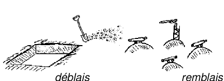
Figure 1: A sketch of Monge’s mass transportation problem in which one searches the optimal way of transporting earth from cuts (déblais) to fills (remblais), each of prescribed shape; the cost of transporting a molecule of earth is a given function of the distance. The MAK method of reconstructing the early Universe described in this paper corresponds to a quadratic cost.

The paper is organized as follows. In Section 2 we formulate the reconstruction problem in an expanding universe and state the main result about uniqueness of the solution.

In the next three sections we devise and test a reconstruction technique called MAK (for Monge–Ampère–Kantorovich) within a restricted framework where the Lagrangian map from initial to present mass locations is taken potential. In Section 3 we discuss the validity of the potentiality assumption and its relation to various approximations used in cosmology; then we derive the Monge–Ampère equation, a simple consequence of mass conservation, introduce its modern reformulation as a Monge–Kantorovich problem of optimal mass transportation and finally discuss different limitations on uniqueness of the reconstruction. In Section 4 we show how discretization turns optimization into an instance of the standard assignment problem; we then present effective algorithms for its solution, foremost the ‘auction’ algorithm of D. Bertsekas. Section 5 is devoted to testing the MAK reconstruction against $N$-body cosmological simulations.

In Section 6, we show how the general case, without the potentiality assumption, can also be recast as an optimization problem with a unique solution and indicate a possible numerical strategy for such reconstruction. In Section 7 we compare our reconstruction method with other approaches in the literature. In Section 8 we discuss perspectives and open problems.

A number of topics are left for appendices. In Appendix A we derive the Eulerian and Lagrangian equations in the form used throughout the paper (and provide some background for non-cosmologists). Appendix B is devoted to the history of optimal mass transportation theory, a subject more than two centuries old (Monge, 1781), which has undergone significant progress within the last two decades. Appendix C is a brief elementary introduction to the technique of duality in optimization, which we use several times throughout the paper. Appendix D gives details of the uniqueness proof that is only outlined in Section 6.

Finally, a word about notation (see also Appendix A). We are using comoving coordinates denoted by ${\mn@boldsymbol{x}}$ in a frame following expansion of the Universe. Our time variable is not the cosmic time but the so-called linear growth factor, here denoted by $\tau$, whose use gives to certain equations the same form as for compressible fluid dynamics in a non-expanding medium. The subscript $0$ refers to the present time (redshift $z=0$), while the quantities evaluated at the initial epoch take the subscript or superscript ‘in.’ Following cosmological usage, the Lagrangian coordinate is denoted ${\mn@boldsymbol{q}}$.

2 Reconstruction in an expanding universe

The most widely accepted explanation of the large-scale structure seen in galaxy surveys is that it results from small primordial fluctuations that grew under gravitational self-interaction of collisionless cold dark matter (CDM) particles in an expanding universe see, e.g., Bernardeau et al. (2002) and references therein. The relevant equations of motion, derived in Appendix A, are the Euler–Poisson equations written here for a flat, matter-dominated Einstein–de Sitter universe (for more general case see, e.g., Catelan et al., 1995):

$${\partial_{\tau}}{\mn@boldsymbol{v}}+({\mn@boldsymbol{v}}\cdot{\nabla_{{\mn@boldsymbol{x}}}}){\mn@boldsymbol{v}} = -\frac{3}{2\tau}({\mn@boldsymbol{v}}+{\nabla_{{\mn@boldsymbol{x}}}}\varphi_{\mathrm{g}}),$$ (1)

$${\partial_{\tau}}\rho+{\nabla_{{\mn@boldsymbol{x}}}}\cdot(\rho{\mn@boldsymbol{v}}) = 0,$$ (2)

$${\nabla^{2}_{{\mn@boldsymbol{x}}}}\varphi_{\mathrm{g}} = \frac{\rho-1}{\tau}.$$ (3)

Here ${\mn@boldsymbol{v}}$ denotes the velocity, $\rho$ denotes the density (normalized by the background density $\bar{\varrho}$) and $\varphi_{\mathrm{g}}$ is a rescaled gravitational potential. All quantities are expressed in comoving spatial coordinates ${\mn@boldsymbol{x}}$ and linear growth factor $\tau$, which is used as the time variable; in particular, ${\mn@boldsymbol{v}}$ is the Lagrangian $\tau$-time derivative of the comoving coordinate of a fluid element.

2.1 Slaving in early-time dynamics and its fossils

The right-hand sides of the momentum and Poisson equations (1) and (3) contain denominators proportional to $\tau$. Hence, a necessary condition for the problem not to be singular as $\tau\to 0$ is

$${\mn@boldsymbol{v}}_{\rm in}({\mn@boldsymbol{x}})+{\nabla_{{\mn@boldsymbol{x}}}}\varphi^{\rm in}_{\rm g}=0,\qquad\rho_{\rm in}({\mn@boldsymbol{x}})=1.$$ (4)

In other words, (i) the initial velocity must be equal to (minus) the gradient of the initial gravitational potential and (ii) the initial normalized mass distribution is uniform. We shall refer to these conditions as slaving. Note that the density contrast $\rho-1$ vanishes initially, but the rescaled gravitational potential and the velocity, as defined here, stay finite thanks to our choice of the linear growth factor as time variable. Therefore we refer to the initial mass distribution as ‘quasi-uniform.’

In the sequel, when we mention the Euler–Poisson initial-value problem, it is always understood that we start at $\tau=0$ and assume slaving. Hence we are extending the Newtonian matter-dominated post-decoupling description back to $\tau=0.$ By examination of the Lagrangian equations for ${\mn@boldsymbol{x}}({\mn@boldsymbol{q}},\tau)$ near $\tau=0$, which can be linearized because the displacement ${\mn@boldsymbol{x}}-{\mn@boldsymbol{q}}$ is small, it is easily shown that slaving implies the absence of the ‘decaying mode,’ which behaves as $\tau^{-3/2}$ in an Einstein–de Sitter universe and is thus singular at $\tau=0$ (for details see Appendix A).

Slaving is also a sufficient condition for the initial problem to be well posed. It is indeed easily shown recursively that (1)–(3) admit a solution in the form of a formal Taylor series in $\tau$ (a related expansion involving only potentials may be found in Catelan et al., 1995):

$${\mn@boldsymbol{v}}({\mn@boldsymbol{x}},\tau) = {\mn@boldsymbol{v}}^{(0)}({\mn@boldsymbol{x}})+\tau{\mn@boldsymbol{v}}^{(1)}({\mn@boldsymbol{x}})+\tau^{2}{\mn@boldsymbol{v}}^{(2)}({\mn@boldsymbol{x}})+\cdots,$$ (5)

$$\varphi_{\mathrm{g}}({\mn@boldsymbol{x}},\tau) = \varphi_{\mathrm{g}}^{(0)}({\mn@boldsymbol{x}})+\tau\varphi_{\mathrm{g}}^{(1)}({\mn@boldsymbol{x}})+\tau^{2}\varphi_{\mathrm{g}}^{(2)}({\mn@boldsymbol{x}})+\cdots,$$ (6)

$$\rho({\mn@boldsymbol{x}},\tau) = 1+\tau\rho^{(1)}({\mn@boldsymbol{x}})+\tau^{2}\rho^{(2)}({\mn@boldsymbol{x}})+\cdots.$$ (7)

Furthermore, ${\mn@boldsymbol{v}}^{(n)}({\mn@boldsymbol{x}})$ is easily shown to be curl-free for any $n$.

Several important consequences of slaving extend to later times as ‘fossils’ of the earliest dynamics. First, as already stressed in the Introduction, the whole dynamics is determined by only one scalar field (e.g., the initial gravitational potential) which we can hope to determine from the knowledge of the present density field.

Second, slaving trivially rules out multi-streaming up to the time of formation of caustics. Since we are working with collisionless matter, the dynamics should in principle be governed by the Vlassov–Poisson kinetic equation which allows at each $({\mn@boldsymbol{x}},\tau)$ point a non-trivial distribution function $f({\mn@boldsymbol{x}},{\mn@boldsymbol{v}},\tau)$. Slaving selects a particular class of solutions for which the distribution function is concentrated on a single-speed manifold, thereby justifying the use of the Euler–Poisson equation without having to invoke any hydrodynamical limit (see, e.g., Vergassola et al., 1994; Catelan et al., 1995).

Third, it is easily checked from (1) that the initial slaved velocity, which is obviously curl-free, remains so for all later times (up to formation of caustics). Note that this vanishing of the curl holds in Eulerian coordinates. A similar property in Lagrangian coordinates can only hold approximately but will play an important role in the sequel (Section 3).

2.2 Formulation of the reconstruction problem

The present Universe is replete with high-density structures: clusters (point-like objects), filaments (line-like objects) and perhaps sheets or walls.

The internal structure of such mass concentrations certainly displays multi-streaming and cannot be described in terms of a single-speed solution to the Euler–Poisson equations. In $N$-body simulations, multi-stream regions are usually found to be of relatively small extension in one or several space directions, typically not more than a few Mpc, and hence have a small volume, although they contain a significant fraction of the total mass (see, e.g. Weinberg & Gunn, 1990).

In order not to have to deal with tiny multi-stream regions, we replace the true mass distribution by a ‘macroscopic’ one which has a regular part and a singular (collapsed) part, the latter concentrated on objects of dimension less than three, such as points or lines.

The general problem of reconstruction is to find as much information as possible on the history of the evolution that carries the initial uniform density into the present macroscopic mass distribution, including the evolution of the velocities. In principle we would like to find a solution of the Euler–Poisson initial-value problem leading to the present density field $\rho_{0}({\mn@boldsymbol{x}})$.

A more restricted problem, which we call the ‘displacement reconstruction,’ is to find the Lagrangian map ${\mn@boldsymbol{q}}\mapsto{\mn@boldsymbol{x}}({\mn@boldsymbol{q}})$ and its inverse ${\mn@boldsymbol{x}}\mapsto{\mn@boldsymbol{q}}({\mn@boldsymbol{x}})$, or in other words to answer the question: where does a given ‘Monge molecule’ of matter originate from? Of course, the inverse Lagrangian map will not be single-valued on mass concentrations. Furthermore, for practical cosmological applications, we define a ‘full reconstruction problem’ as (i) displacement reconstruction and (ii) obtaining the initial and present peculiar velocity fields, ${\mn@boldsymbol{v}}_{\rm in}({\mn@boldsymbol{q}})$ and ${\mn@boldsymbol{v}}_{0}({\mn@boldsymbol{x}})$.

We shall show in this paper that the displacement reconstruction problem is uniquely solvable and that the full reconstruction problem has a unique solution outside of mass concentrations; as to the latter, they are traced back to collapsed regions in the Lagrangian space whose shape and positions are well defined but the inner structure of density and velocity fluctuations is irretrievably lost.

3 Potential Lagrangian maps: the MAK reconstruction

In this and the next two sections we shall assume that the Lagrangian map from initial positions to present ones is potential

$${\mn@boldsymbol{x}}=\nabla_{{\mn@boldsymbol{q}}}\Phi({\mn@boldsymbol{q}}),$$ (8)

and furthermore that the potential $\Phi({\mn@boldsymbol{q}})$ is convex, which is, as we shall see, related to the absence of multi-streaming.

3.1 Approximations leading to maps with convex potentials

The motivation for the potential assumption, first used by Bertschinger & Dekel (1989), comes from the Zel’dovich approximation (Zel’dovich, 1970), denoted here by ZA, and its refinements. To recall how the ZA comes about, let us start from the equations for the Lagrangian map ${\mn@boldsymbol{x}}({\mn@boldsymbol{q}},\tau)$, written in the Lagrangian coordinate ${\mn@boldsymbol{q}}$ (Appendix A)

$${D^{2}_{\tau}}{\mn@boldsymbol{x}} = -\frac{3}{2\tau}({D_{\tau}}{\mn@boldsymbol{x}}+{\nabla_{{\mn@boldsymbol{x}}}}\varphi_{\mathrm{g}}),$$ (9)

$${\nabla^{2}_{{\mn@boldsymbol{x}}}}\varphi_{\mathrm{g}} = \frac{1}{\tau}\left[\left(\det{\nabla_{{\mn@boldsymbol{q}}}}{\mn@boldsymbol{x}}\right)^{-1}-1\right],$$ (10)

where ${D_{\tau}}$ is the Lagrangian time derivative and $\nabla_{x_{i}}\equiv(\partial{q_{j}}/\partial{x_{i}})\nabla_{q_{j}}$ is the Eulerian gradient rewritten in Lagrangian coordinates. As shown in Appendix A, in one space dimension the Hubble drag term ${D_{\tau}}{\mn@boldsymbol{x}}$ and the gravitational acceleration term ${\nabla_{{\mn@boldsymbol{x}}}}\varphi_{\mathrm{g}}$ cancel exactly. Slaving, discussed in Section 2.1, means that the same cancellation holds to leading order in any dimension for small $\tau$. The ZA extends this as an approximation without the restriction of small $\tau$. Within the ZA, the acceleration ${D^{2}_{\tau}}{\mn@boldsymbol{x}}$ vanishes. Hence the Lagrangian map has the form

$${\mn@boldsymbol{x}}({\mn@boldsymbol{q}},\tau) = {\mn@boldsymbol{q}}+\tau({D_{\tau}}{\mn@boldsymbol{x}})_{\rm in}({\mn@boldsymbol{q}})={\mn@boldsymbol{q}}-\tau{\nabla_{{\mn@boldsymbol{q}}}}\varphi^{\rm in}_{\rm g}({\mn@boldsymbol{q}})$$

$$= {\nabla_{{\mn@boldsymbol{q}}}}\Phi({\mn@boldsymbol{q}},\tau)$$

with the potential

$$\Phi({\mn@boldsymbol{q}},\tau)\equiv\frac{|{\mn@boldsymbol{q}}|^{2}}{2}-\tau\varphi^{\rm in}_{\rm g}({\mn@boldsymbol{q}}).$$ (12)

Furthermore, taking the time derivative of (3.1), we see that the velocity ${D_{\tau}}{\mn@boldsymbol{x}}({\mn@boldsymbol{q}},\tau)$ is curl-free with respect to the Lagrangian coordinate ${\mn@boldsymbol{q}}$.

Potentiality of the Lagrangian map (and consequently the Lagrangian potentiality of the velocity) is perhaps the most important feature of the ZA. Unlike the vanishing of the acceleration, it does not depend on the choice of the linear growth factor as the time variable. However, unaccelerated but vortical flow would fail to exhibit the cancellation necessary for the ZA to hold. It is noteworthy that the potentiality is not limited to the ZA: indeed, the latter can be formulated as the first order of a systematic Lagrangian perturbation theory in which, up to second order, the Lagrangian map is still potential under slaving Moutarde et al., 1991; Buchert, 1992; Buchert & Ehlers, 1993; Munshi, Sahni & Starobinsky, 1994; Catelan, 1995.

It is well known that the ZA map defined by (3.1) ceases in general to be invertible due to the formation of multi-stream regions bounded by caustics. Since particles move along straight lines in the ZA, the formation of caustics proceeds just as in ordinary optics in a uniform medium in which light rays are also straight. One of the problems with the ZA is that caustics, which start as localized objects, quickly grow in size and give unrealistically large multi-stream regions.

A modification of the ZA that has no multi-streaming at all, but sharp mass concentrations in the form of shocks and other singularities, has been introduced by Gurbatov & Saichev 1984; Gurbatov et al., 1989; Shandarin & Zel’dovich, 1989, see also. It is known as the adhesion model. In Eulerian coordinates it amounts to using a multidimensional Burgers equation (see, e.g., Frisch & Bec, 2002)

$${\partial_{\tau}}{\mn@boldsymbol{v}}+({\mn@boldsymbol{v}}\cdot{\nabla_{{\mn@boldsymbol{x}}}}){\mn@boldsymbol{v}}=\nu{\nabla^{2}_{{\mn@boldsymbol{x}}}}{\mn@boldsymbol{v}},\qquad{\mn@boldsymbol{v}}=-{\nabla_{{\mn@boldsymbol{x}}}}\varphi_{\mathrm{v}},$$ (13)

taken in the limit where the viscosity $\nu$ tends to zero. In Lagrangian coordinates, the adhesion model is obtained from the ZA by replacing the velocity potential $\Phi({\mn@boldsymbol{q}},t)$ given by (12) by its convex hull $\Phi_{c}({\mn@boldsymbol{q}},t)$ in the ${\mn@boldsymbol{q}}$ variable (Vergassola et al., 1994).

Convexity is a concept which plays an important role in this paper, and a few words on it are in order here (see also Appendix C.1). A body in the three-dimensional space is said to be convex if, whenever it contains two points, it contains also the whole segment joining them. A function $f({\mn@boldsymbol{q}})$ is said to be convex if the set of all points lying above its graph is convex. The convex hull of the function $\Phi({\mn@boldsymbol{q}})$ is defined as the largest convex function whose graph lies below that of $\Phi({\mn@boldsymbol{q}})$. In two dimensions it can be visualized by wrapping the graph of $\Phi({\mn@boldsymbol{q}})$ tightly from below with an elastic sheet.

Note that $\Phi({\mn@boldsymbol{q}},\tau)$ given by (12) is obviously convex for small enough $\tau$ since it is then very close to the parabolic function $|{\mn@boldsymbol{q}}|^{2}/2$. After caustics form, convexity is lost in the ZA but recovered with the adhesion model. It may then be shown that those regions in the Lagrangian space where $\Phi({\mn@boldsymbol{q}},t)$ does not coincide with its convex hull will be mapped in the Eulerian space to sheets, lines and points, each of which contains a finite amount of mass. At these locations the Lagrangian map does not have a uniquely defined Lagrangian antecedent but such points form a set of vanishing volume. Everywhere else, there is a unique antecedent and hence no multi-streaming.

Although the adhesion model has a number of known shortcomings, such as non-conservation of momentum in more than one dimension, it has been found to be in better agreement with $N$-body simulations than the ZA (Weinberg & Gunn, 1990). Other single-speed approximations to multi-stream flow, overcoming difficulties of the adhesion model, are discussed e.g. by Shandarin & Sathyaprakash (1996); Buchert & Dominguez (1998); Fanelli & Aurell (2002). In such models, multi-streaming is completely suppressed by a mechanism of momentum exchange between neighbouring streams with different velocities. This is of course a common phenomenon in ordinary fluids, where it is due to viscous diffusion; dark matter is however essentially collisionless and the usual mechanism for generating viscosity does not operate, so that a non-collisional mechanism must be invoked. A qualitative explanation using the modification of the gravitational forces after the formation of caustics has been proposed by Shandarin & Zel’dovich (1989). In our opinion the mechanism limiting multi-streaming to rather narrow regions is poorly understood and deserves considerable further investigation.

3.2 The Monge–Ampère equation: a consequence of mass conservation and potentiality

We now show that the assumption that the Lagrangian map is derived from a convex potential leads to a pair of non-linear partial differential equations, one for this potential and another for its Legendre transform.

Let us first assume that the present distribution of mass has no singular part, an assumption which we shall relax later. Since in our notation the initial quasi-uniform mass distribution has unit density, mass conservation implies $\rho_{0}({\mn@boldsymbol{x}})\,\mathrm{d}^{3}{\mn@boldsymbol{x}}=\mathrm{d}^{3}{\mn@boldsymbol{q}}$, which can be rewritten in terms of the Jacobian matrix ${\nabla_{{\mn@boldsymbol{q}}}}{\mn@boldsymbol{x}}$ as

$$\det{\nabla_{{\mn@boldsymbol{q}}}}{\mn@boldsymbol{x}}=\frac{1}{\rho_{0}({\mn@boldsymbol{x}}({\mn@boldsymbol{q}}))}.$$ (14)

Under the potential assumption (8), this takes the form

$$\det(\nabla_{q_{i}}\nabla_{q_{j}}\Phi({\mn@boldsymbol{q}}))=\frac{1}{\rho_{0}\bigl{(}{\nabla_{{\mn@boldsymbol{q}}}}\Phi({\mn@boldsymbol{q}})\bigr{)}}.$$ (15)

A similar equation follows also from Eqs. (1) and (2) of Bertschinger & Dekel (1989).

A simpler equation, in which the unknown appears only in the left-hand side, viz Eq. (19) below, is obtained for the potential of the inverse Lagrangian map ${\mn@boldsymbol{q}}({\mn@boldsymbol{x}})$. Key is the observation that the inverse of a map with a convex potential has also a convex potential, and that the two potentials are Legendre transforms of each other. A purely local proof of this statement is to observe that potentiality of ${\mn@boldsymbol{q}}({\mn@boldsymbol{x}})$ is equivalent to the symmetry of the inverse Jacobian matrix ${\nabla_{{\mn@boldsymbol{x}}}}{\mn@boldsymbol{q}}$ which follows because it is the inverse of the symmetrical matrix ${\nabla_{{\mn@boldsymbol{q}}}}{\mn@boldsymbol{x}}$; convexity is equivalent to the positive-definiteness of these matrices. Obviously the function

$$\Theta({\mn@boldsymbol{x}})\equiv{\mn@boldsymbol{x}}\cdot{\mn@boldsymbol{q}}({\mn@boldsymbol{x}})-\Phi({\mn@boldsymbol{q}}({\mn@boldsymbol{x}})),$$ (16)

which is the Legendre transform of $\Phi({\mn@boldsymbol{q}})$, is the potential for the inverse Lagrangian map. The modern definition of the Legendre transformation (see Appendix C.1), needed for generalization to non-smooth mass distributions, is

$$\Theta({\mn@boldsymbol{x}}) = \max_{\mn@boldsymbol{q}}\,{\mn@boldsymbol{x}}\cdot{\mn@boldsymbol{q}}-\Phi({\mn@boldsymbol{q}}),$$ (17)

$$\Phi({\mn@boldsymbol{q}}) = \max_{\mn@boldsymbol{x}}\,{\mn@boldsymbol{x}}\cdot{\mn@boldsymbol{q}}-\Theta({\mn@boldsymbol{x}}).$$ (18)

In terms of the potential $\Theta$, mass conservation is immediately written as

$$\det(\nabla_{x_{i}}\nabla_{x_{j}}\Theta({\mn@boldsymbol{x}}))=\rho_{0}({\mn@boldsymbol{x}}).$$ (19)

This equation, which has the determinant of the second derivatives of the unknown in the left-hand side and a prescribed (positive) function in the right-hand side, is called the (elliptic) Monge–Ampère equation (see Appendix B for a historical perspective).

Notice that our Monge–Ampère equation may be viewed as a non-linear generalization of the Poisson equation (used for reconstruction by Nusser & Dekel (1992); see also Section 7.1), to which it reduces if particles have moved very little from their initial positions.

In actual reconstructions we have to deal with mass concentration in the present distribution of matter. Thus the density in the right-hand side of (19) has a singular component (a Dirac distribution concentrated on sets carrying the concentrated mass) and the potential $\Theta$ ceases to be smooth. As we now show, a generalized meaning can nevertheless be given to the Monge–Ampère equation by using the key ingredient in its derivation, namely mass conservation, in integrated form.

For a nonsmooth convex potential $\Theta$, taking the gradient ${\nabla_{{\mn@boldsymbol{x}}}}\Theta({\mn@boldsymbol{x}})$ still makes sense if one allows it to be multivalued at points where the potential is not differentiable. The gradient at such a point ${\mn@boldsymbol{x}}$ is then the set of all possible slopes of planes touching the graph of $\Theta$ at $({\mn@boldsymbol{x}},\Theta({\mn@boldsymbol{x}}))$ (this idea is given a precise mathematical formulation in Appendix C.1). As ${\mn@boldsymbol{x}}$ varies over an arbitrary domain $\mathcal{D}_{\mathrm{E}}$ in the Eulerian space, its image ${\mn@boldsymbol{q}}({\mn@boldsymbol{x}})$ sweeps a domain ${\mn@boldsymbol{q}}(\mathcal{D}_{\mathrm{E}})$ in the Lagrangian space, and mass conservation requires that

$$\int_{\mathcal{D}_{\mathrm{E}}}\rho_{0}({\mn@boldsymbol{x}})\,\mathrm{d}^{3}{\mn@boldsymbol{x}}=\int_{{\nabla_{{\mn@boldsymbol{x}}}}\Theta(\mathcal{D}_{\mathrm{E}})}\mathrm{d}^{3}{\mn@boldsymbol{q}},$$ (20)

where we take into account that ${\mn@boldsymbol{q}}({\mn@boldsymbol{x}})={\nabla_{{\mn@boldsymbol{x}}}}\Theta({\mn@boldsymbol{x}})$. Eq. (20) must hold for any Eulerian domain $\mathcal{D}_{\mathrm{E}}$; this requirement is known as the weak formulation of the Monge–Ampère equation (19). A symmetric formulation may be written for (15) in terms of ${\mn@boldsymbol{x}}({\mn@boldsymbol{q}})={\nabla_{{\mn@boldsymbol{q}}}}\Phi({\mn@boldsymbol{q}})$. For further material on the weak formulation see, e.g., Pogorelov (1978).

Considerable literature has been devoted to the Monge–Ampère equation in recent years (see, e.g., Caffarelli, 1999; Caffarelli & Milman, 1999). We mention now a few results which are of direct relevance for the reconstruction problem.

In a nutshell, one can prove that when the domains occupied by the mass initially and at present are bounded and convex, the Monge–Ampère equation – in its weak formulation – is guaranteed to have a unique solution, which is smooth unless one or both of the mass distributions is non-smooth. The actual construction of this solution can be done by a variational method discussed in the next section.

A similar result holds also when the present density field is periodic and the same periodicity is assumed for the map.

Also relevant, as we shall see in Section 3.4, is a recent result of Caffarelli & Li (2001): if the Monge–Ampère equation is considered in the whole space, but the present density contrast $\delta=\rho-1$ vanishes outside of a bounded set, then the solution $\Theta({\mn@boldsymbol{x}})$ is determined uniquely up to prescription of its asymptotic behaviour at infinity, which is specified by a quadratic function of the form

$$\theta({\mn@boldsymbol{x}})\equiv\langle{\mn@boldsymbol{x}},A{\mn@boldsymbol{x}}\rangle+\langle\mn@boldsymbol{b},{\mn@boldsymbol{x}}\rangle+c,$$ (21)

for some positive definite symmetric matrix $A$ with unit determinant, vector $\mn@boldsymbol{b}$ and constant $c$.

3.3 Optimal mass transportation

As we are going to see now, the Monge–Ampère equation (19) is equivalent to an instance of what is called the ‘optimal mass transportation problem.’ Suppose we are given two distributions $\rho_{\rm in}({\mn@boldsymbol{q}})$ and $\rho_{0}({\mn@boldsymbol{x}})$ of the same amount of mass in two three-dimensional convex bounded domains ${\cal D}_{\rm in}$ and ${\cal D}_{0}$. The optimal mass transportation problem is then to find the most cost-effective way of rearranging by a suitable map one distribution into the other, the cost of transporting a unit of mass from a position ${\mn@boldsymbol{q}}\in{\cal D}_{\rm in}$ to ${\mn@boldsymbol{x}}\in{\cal D}_{0}$ being a prescribed function $c({\mn@boldsymbol{q}},{\mn@boldsymbol{x}})$.

Denoting the map by ${\mn@boldsymbol{x}}({\mn@boldsymbol{q}})$ and its inverse ${\mn@boldsymbol{q}}({\mn@boldsymbol{x}})$, we can write the problem as the requirement that the cost

$$I\equiv\int_{{\cal D}_{\rm in}}\!\!\!c({\mn@boldsymbol{q}},{\mn@boldsymbol{x}}({\mn@boldsymbol{q}}))\rho_{\rm in}({\mn@boldsymbol{q}})\,\mathrm{d}^{3}{\mn@boldsymbol{q}}=\int_{{\cal D}_{0}}\!\!\!c({\mn@boldsymbol{q}}({\mn@boldsymbol{x}}),{\mn@boldsymbol{x}})\rho_{0}({\mn@boldsymbol{x}})\,\mathrm{d}^{3}{\mn@boldsymbol{x}}$$ (22)

be minimum, with the constraints of prescribed ‘terminal’ densities $\rho_{\rm in}$ and $\rho_{0}$ and of mass conservation $\rho_{\rm in}({\mn@boldsymbol{q}})\,\mathrm{d}^{3}{\mn@boldsymbol{q}}=\rho_{0}({\mn@boldsymbol{x}})\,\mathrm{d}^{3}{\mn@boldsymbol{x}}$.

This problem goes back to Monge (1781) who considered the case of a linear cost function $c({\mn@boldsymbol{q}},{\mn@boldsymbol{x}})=|{\mn@boldsymbol{x}}-{\mn@boldsymbol{q}}|$ (see Appendix B and Fig. 1).

For our purposes, the central result is that the problem of finding a potential Lagrangian map with presecribed initial and present mass density fields is equivalent to a mass transportation problem with quadratic cost. Indeed, it is known (Brenier, 1987, 1991) that, when the cost is a quadratic function of the distance, so that

$$I=\!\int_{{\cal D}_{\rm in}}\!\!\!\!\frac{|{\mn@boldsymbol{x}}({\mn@boldsymbol{q}})-{\mn@boldsymbol{q}}|^{2}\!\!\!}{2}\,\rho_{\rm in}({\mn@boldsymbol{q}})\,\mathrm{d}^{3}{\mn@boldsymbol{q}}=\!\int_{{\cal D}_{0}}\!\!\!\!\frac{|{\mn@boldsymbol{x}}-{\mn@boldsymbol{q}}({\mn@boldsymbol{x}})|^{2}\!\!\!}{2}\,\rho_{0}({\mn@boldsymbol{x}})\,\mathrm{d}^{3}{\mn@boldsymbol{x}},$$ (23)

the solution ${\mn@boldsymbol{q}}({\mn@boldsymbol{x}})$ to the optimal mass transportation problem is the gradient of a convex function, which then must satisfy the Monge–Ampère equation (19) by mass conservation.

A particularly simple variational proof can be given for the smooth case, when the two mutually inverse maps ${\mn@boldsymbol{x}}({\mn@boldsymbol{q}})$ and ${\mn@boldsymbol{q}}({\mn@boldsymbol{x}})$ are both well defined.

Performing a variation of the map ${\mn@boldsymbol{x}}({\mn@boldsymbol{q}})$, we cause a mass element in the Eulerian space that was located at ${\mn@boldsymbol{x}}({\mn@boldsymbol{q}})$ to move to ${\mn@boldsymbol{x}}({\mn@boldsymbol{q}})+\delta{\mn@boldsymbol{x}}({\mn@boldsymbol{q}})$. This variation is constrained not to change the density field $\rho_{0}$. To express this constraint it is convenient to rewrite the displacement in Eulerian coordinate $\delta{\mn@boldsymbol{x}}_{\rm E}({\mn@boldsymbol{x}})\equiv\delta{\mn@boldsymbol{x}}({\mn@boldsymbol{q}}({\mn@boldsymbol{x}}))$. Noting that the point ${\mn@boldsymbol{x}}$ gets displaced into ${\mn@boldsymbol{y}}={\mn@boldsymbol{x}}+\delta{\mn@boldsymbol{x}}$, we thus require that $\rho_{0}({\mn@boldsymbol{x}})\,\mathrm{d}^{3}{\mn@boldsymbol{x}}=\rho_{0}({\mn@boldsymbol{y}})\,\mathrm{d}^{3}{\mn@boldsymbol{y}}$ or

$$\rho_{0}({\mn@boldsymbol{x}})=\rho_{0}({\mn@boldsymbol{x}}+\delta{\mn@boldsymbol{x}}_{\mathrm{E}}({\mn@boldsymbol{x}}))\,\det\bigl{(}{\nabla_{{\mn@boldsymbol{x}}}}({\mn@boldsymbol{x}}+\delta{\mn@boldsymbol{x}}_{\mathrm{E}}({\mn@boldsymbol{x}}))\bigr{)}.$$ (24)

Expanding this equation, we find that, to the leading order,

$${\nabla_{{\mn@boldsymbol{x}}}}\cdot\left(\rho_{0}({\mn@boldsymbol{x}})\,\delta{\mn@boldsymbol{x}}_{\rm E}({\mn@boldsymbol{x}})\right)=0,$$ (25)

an equation which just expresses the physically obvious fact that the mass flux $\rho_{0}({\mn@boldsymbol{x}})\,\delta{\mn@boldsymbol{x}}_{\rm E}({\mn@boldsymbol{x}})$ should have zero divergence. Performing the variation on the functional $I$ given by (23), we get

$$\delta I = \int_{\mathcal{D}_{\mathrm{in}}}({\mn@boldsymbol{x}}({\mn@boldsymbol{q}})-{\mn@boldsymbol{q}})\cdot\delta{\mn@boldsymbol{x}}({\mn@boldsymbol{q}})\,\rho_{\mathrm{in}}({\mn@boldsymbol{q}})\,\mathrm{d}^{3}{\mn@boldsymbol{q}}$$ (26)

$$= \int_{\mathcal{D}_{0}}({\mn@boldsymbol{x}}-{\mn@boldsymbol{q}}({\mn@boldsymbol{x}}))\cdot\bigl{(}\rho_{0}({\mn@boldsymbol{x}})\,\delta{\mn@boldsymbol{x}}_{\mathrm{E}}({\mn@boldsymbol{x}})\bigr{)}\,\mathrm{d}^{3}{\mn@boldsymbol{x}}=0,$$

which has to hold under the constraint (25). In other words, the displacement ${\mn@boldsymbol{x}}-{\mn@boldsymbol{q}}({\mn@boldsymbol{x}})$ has to be orthogonal (in the $L_{2}$ functional sense) to all divergence-less vector fields and, thus, must be a gradient. Since ${\mn@boldsymbol{x}}$ is obviously a gradient, it follows that ${\mn@boldsymbol{q}}({\mn@boldsymbol{x}})={\nabla_{{\mn@boldsymbol{x}}}}\Theta({\mn@boldsymbol{x}})$ for a suitable potential $\Theta$.

It remains to prove the convexity of $\Theta$. First we prove that the map ${\mn@boldsymbol{x}}\mapsto{\mn@boldsymbol{q}}({\mn@boldsymbol{x}})={\nabla_{{\mn@boldsymbol{x}}}}\Theta({\mn@boldsymbol{x}})$ is monotone, i.e., by definition, that for any ${\mn@boldsymbol{x}}_{1}$ and ${\mn@boldsymbol{x}}_{2}$

$$({\mn@boldsymbol{x}}_{2}-{\mn@boldsymbol{x}}_{1})\cdot({\mn@boldsymbol{q}}({\mn@boldsymbol{x}}_{2})-{\mn@boldsymbol{q}}({\mn@boldsymbol{x}}_{1}))\geq 0.$$ (27)

Indeed, should this inequality be violated for some $\overline{{\mn@boldsymbol{x}}}_{1},\overline{{\mn@boldsymbol{x}}}_{2}$, the continuity of ${\mn@boldsymbol{q}}({\mn@boldsymbol{x}})$ would imply that for all ${\mn@boldsymbol{x}}_{1},{\mn@boldsymbol{x}}_{2}$ close enough to $\overline{{\mn@boldsymbol{x}}}_{1},\overline{{\mn@boldsymbol{x}}}_{2}$

$$\begin{array}[]{l}\displaystyle|{\mn@boldsymbol{q}}({\mn@boldsymbol{x}}_{1})-{\mn@boldsymbol{x}}_{1}|^{2}+|{\mn@boldsymbol{q}}({\mn@boldsymbol{x}}_{2})-{\mn@boldsymbol{x}}_{2}|^{2}\\[6.45831pt] \displaystyle\quad>|{\mn@boldsymbol{q}}({\mn@boldsymbol{x}}_{2})-{\mn@boldsymbol{x}}_{1}|^{2}+|{\mn@boldsymbol{q}}({\mn@boldsymbol{x}}_{1})-{\mn@boldsymbol{x}}_{2}|^{2}.\end{array}$$ (28)

This in turn means that if we interchange the destinations of small patches around $\overline{{\mn@boldsymbol{x}}}_{1}$ and $\overline{{\mn@boldsymbol{x}}}_{2}$, sending them not to the corresponding patches around ${\mn@boldsymbol{q}}(\overline{{\mn@boldsymbol{x}}}_{1})$ and ${\mn@boldsymbol{q}}(\overline{{\mn@boldsymbol{x}}}_{2})$ but vice versa, then the value of the functional $I$ will decrease by a small yet positive quantity, and therefore it cannot be minimum for the original map.

To complete the argument, observe that convexity of a smooth function $\Theta({\mn@boldsymbol{x}})$ follows if the matrix of its second derivatives $\nabla_{x_{i}}\nabla_{x_{j}}\Theta({\mn@boldsymbol{x}})$ is positive definite for all ${\mn@boldsymbol{x}}$. Substituting ${\mn@boldsymbol{q}}({\mn@boldsymbol{x}})={\nabla_{{\mn@boldsymbol{x}}}}\Theta({\mn@boldsymbol{x}})$ into (27), assuming that ${\mn@boldsymbol{x}}_{2}$ is close to ${\mn@boldsymbol{x}}_{1}$ and Taylor expanding, we find that

$$({\mn@boldsymbol{x}}_{2}-{\mn@boldsymbol{x}}_{1})\cdot(\nabla_{x_{i}}\nabla_{x_{j}}\Theta({\mn@boldsymbol{x}}_{1})\,({\mn@boldsymbol{x}}_{2}-{\mn@boldsymbol{x}}_{1}))\geq 0.$$ (29)

As ${\mn@boldsymbol{x}}_{2}$ is arbitrary, this proves the desired positive definiteness and thus establishes the equivalence of the Monge–Ampère equation (19) and of the mass transportation problem with quadratic cost.

This equivalence is actually proved under much weaker conditions, not requiring any smoothness (Brenier, 1987, 1991). The proof makes use of the ‘relaxed’ reformulation of the mass transportation problem due to Kantorovich (1942). Instead of solving the highly non-linear problem of finding a map ${\mn@boldsymbol{q}}({\mn@boldsymbol{x}})$ minimizing the cost (22) with prescribed terminal densities, Kantorovich considered the linear programming problem of minimizing

$$\tilde{I}\equiv\int_{\mathcal{D}_{\mathrm{in}}}\!\!\int_{\mathcal{D}_{0}}c({\mn@boldsymbol{q}},{\mn@boldsymbol{x}})\,\rho({\mn@boldsymbol{q}},{\mn@boldsymbol{x}})\,\mathrm{d}^{3}{\mn@boldsymbol{q}}\,\mathrm{d}^{3}{\mn@boldsymbol{x}},$$ (30)

under the constraint that the joint distribution $\rho({\mn@boldsymbol{q}},{\mn@boldsymbol{x}})$ is nonnegative and has marginals $\rho_{\mathrm{in}}({\mn@boldsymbol{q}})$ and $\rho_{0}({\mn@boldsymbol{x}})$, the latter being equivalent to

$$\int_{\mathcal{D}_{0}}\rho({\mn@boldsymbol{q}},{\mn@boldsymbol{x}})\,\mathrm{d}^{3}{\mn@boldsymbol{x}}=\rho_{\mathrm{in}}({\mn@boldsymbol{q}}),\quad\int_{\mathcal{D}_{\mathrm{in}}}\rho({\mn@boldsymbol{q}},{\mn@boldsymbol{x}})\,\mathrm{d}^{3}{\mn@boldsymbol{q}}=\rho_{0}({\mn@boldsymbol{x}}).$$ (31)

Note that if we assume any of the two following forms for the joint distribution

$$\begin{array}[]{l}\rho({\mn@boldsymbol{q}},{\mn@boldsymbol{x}})=\rho_{0}({\mn@boldsymbol{x}})\,\delta\bigl{(}{\mn@boldsymbol{q}}-{\mn@boldsymbol{q}}({\mn@boldsymbol{x}})\bigr{)}\\[4.30554pt] \rho({\mn@boldsymbol{q}},{\mn@boldsymbol{x}})=\rho_{\rm in}({\mn@boldsymbol{q}})\,\delta\bigl{(}{\mn@boldsymbol{x}}-{\mn@boldsymbol{x}}({\mn@boldsymbol{q}})\bigr{)},\end{array}$$ (32)

we find that $\tilde{I}$ reduces to the cost $I$ as defined in (22). This relaxed formulation allowed Kantorovich to establish the existence of a mimimizing joint distribution.

The relaxed formulation can be used to show that the minimizing solution actually defines a map, which need not be smooth if one or both of the terminal distribution have a singular component (in our case, when mass concentrations are present). The derivation (Brenier, 1987, 1991) makes use of the technique of duality (Appendix C.2), which will also appear in discussing algorithms (Section 4.2) and reconstruction beyond the potential hypothesis (Section 6).

We have thus shown that the Monge–Kantorovich optimal mass transportation problem can be applied to solving the Monge–Ampère equation. The actual implementation (Section 4), done for a suitable discretization, will be henceforth called Monge–Ampère–Kantorovich (MAK).

3.4 Sources of uncertainty in reconstruction

In this section we discuss various sources of non-uniqueness of the MAK reconstruction: multi-streaming, collapsed regions, reconstruction from a finite patch of the Universe.

We have stated before that our uniqueness result applies only in so far as we can treat present-epoch high-density multi-stream regions as if they were truly collapsed, ignoring their width. We now give a simple one-dimensional example of non-uniqueness in which a thick region of multi-streaming is present. Fig. 2 shows a multi-stream Lagrangian map $x(q)$ and the associated density distribution; the inverse map $q(x)$ is clearly multi-valued. The same density distribution may however be generated by a spurious single-stream Lagrangian map shown on the same figure. There is no way to distinguish between the two inverse Lagrangian maps if the various streams cannot be disentangled.

Figure 2: A one-dimensional example of non-unique reconstruction of the Lagrangian map in the presence of multi-streaming. The density distribution (upper graph) is generated by a multi-streaming Lagrangian map (thick line of lower graph) but may also be generated by a spurious single-stream Lagrangian map (dashed line).

Suppose now that the present density has a singular part, i.e. there are mass concentrations present which have vanishing (Eulerian) volumes but possess finite masses. Obviously any such object originates from a domain in the Lagrangian space which occupies a finite volume. A one-dimensional example is again helpful. Fig. 3 shows a Lagrangian map in which a whole Lagrangian shock interval $[q_{1},q_{2}]$ has collapsed into a single point of the $x$ axis. Outside of this point the Lagrangian map is uniquely invertible but the point itself has many antecedents. Note that the graph of the Lagrangian map may be inverted by just interchanging the $q$ and $x$ axes, but its inverse contains a piece of vertical line. The position of the Lagrangian shock interval which has collapsed by the present epoch is uniquely defined by the present mass field but the initial velocity fluctuations in this interval cannot be uniquely reconstructed. In particular there is no way to know if collapse has started before the present epoch. We can of course arbitrarily assume that collapse has just happened at the present epoch; if we also suppose that particles have travelled with a constant speed, i.e. use the Zel’dovich/adhesion approximation, then the initial velocity profile within the Lagrangian shock interval will be linear (Fig. 3). Any other smooth velocity profile joining the same end points would have points where its slope (velocity gradient) is more negative than that of the linear profile (Fig. 3) and thus would have started collapse before the present epoch (in one dimension caustics appear at the time which is minus the inverse of the most negative initial velocity gradient).

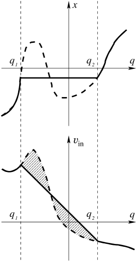
Figure 3: Two initial velocity profiles $v_{\mathrm{in}}(q)$ (bottom, solid and dashed lines) leading to the same Lagrangian map $x=q+\tau v_{\mathrm{in}}(q)$ (top, solid line) in the adhesion approximation. The Zel’dovich approximation would give multistreaming (top, dashed line). Hatched areas (bottom) are equal in the adhesion dynamics.

All this carries over to more than one dimension. The MAK reconstruction gives a unique antecedent for any Eulerian position outside mass concentrations. Each mass concentration in the Eulerian space, taken globally, has a uniquely defined Lagrangian antecedent region but the initial velocity field inside the latter is unknown. In other words, displacement reconstruction is well defined but full reconstruction, based on the Zel’dovich/adhesion approximation for velocities, is possible only outside of mass concentrations (note however that velocities in the Eulerian space are still reconstructed at almost all points). We call the corresponding initial Lagrangian domains collapsed regions.

Finally, we consider a uniqueness problem arising from knowing the present mass distribution only truncated over a finite Eulerian domain ${\cal D}_{0}$, as is necessarily the case when working with a real catalogue. If we also know the corresponding Lagrangian domain ${\cal D}_{\mathrm{in}}$ and both domains are bounded and convex, then uniqueness is guaranteed (see Section 3.2). What we know for sure about ${\cal D}_{\mathrm{in}}$ is its volume, which (in our units) is equal to the total mass contained in ${\cal D}_{0}$. Its shape and position may however be constrained by further information. For example, if we know that the typical displacement of mass elements since decoupling is about ten Mpc in comoving coordinates (see Section 5) and our data extend over a patch of typical size one hundred Mpc, then there is not more than a ten percent uncertainty on the shape of ${\cal D}_{\mathrm{in}}$. Additional information about peculiar velocities may also be used to constrain ${\cal D}_{\mathrm{in}}$.

Note also that a finite-size patch ${\cal D}_{0}$ with unknown antecedent ${\cal D}_{\mathrm{in}}$ will give rise to a unique reconstruction (up to a translation) if we assume that it is surrounded by a uniform background extending to infinity. This is a consequence of the result of Caffarelli & Li mentioned at the end of Section 3.2. The arbitrary linear term in (21) corresponds to a translation; as to the quadratic term, it is constrained by the cosmological principle of isotropy to be exactly $|{\mn@boldsymbol{q}}|^{2}/2$.

4 The MAK method: discretization and algorithmics

In this section we show how to compute the solution to the Monge–Ampère–Kantorovich (MAK) problem the known present density field. First the problem is discretized into an assignment problem (Section 4.1), then we present some general tools which make the assignment problem computationally tractable (Section 4.2) and finally we present, to the best of our knowledge, the most effective method for solving our particular assignment problem, based on the auction algorithm of D. Bertsekas (Section 4.3), and details of its implementation for the MAK reconstruction (Section 4.4).

4.1 Reduction to an assignment problem

Perhaps the most natural way of discretizing a spatial mass distribution is to approximate it by a finite system of identical Dirac point masses, with possibly more than one mass at a given location. This is compatible both with $N$-body simulations and with the intrinsically discrete nature of observed luminous matter. Assuming that we have $N$ unit masses both in the Lagrangian and the Eulerian space, we may write

$$\rho_{0}({\mn@boldsymbol{x}})=\sum_{i=1}^{N}\delta({\mn@boldsymbol{x}}-{\mn@boldsymbol{x}}_{i}),\qquad\rho_{\mathrm{in}}({\mn@boldsymbol{q}})=\sum_{j=1}^{N}\delta({\mn@boldsymbol{q}}-{\mn@boldsymbol{q}}_{j}).$$ (33)

For discrete densities of this form, the mass conservation constraint in the optimal mass transportation problem (Section 3.3) requires that the map ${\mn@boldsymbol{q}}({\mn@boldsymbol{x}})$ induce a one-to-one pairing between positions of the unit masses in the ${\mn@boldsymbol{x}}$ and ${\mn@boldsymbol{q}}$ spaces, which may be written as a permutation of indices that sends ${\mn@boldsymbol{x}}_{i}$ to ${\mn@boldsymbol{q}}_{j(i)}$. Substituting this into the quadratic cost functional (23), we get

$$I=\sum_{i=1}^{N}\frac{|{\mn@boldsymbol{x}}_{i}-{\mn@boldsymbol{q}}_{j(i)}|^{2}}{2}.$$ (34)

We thus reduced the problem to the purely combinatorial one of finding a permutation $j(i)$ (or its inverse $i(j)$) that minimizes the quadratic cost function (34).

This problem is an instance of the general assignment problem in combinatorial optimization: for a cost matrix $c_{ij}$, find a permutation $j(i)$ that minimizes the cost function

$$I=\sum_{i=1}^{N}c_{i\,j(i)}.$$ (35)

As we shall see in the next sections, there exist effective algorithms for finding minimizing permutations.

Before proceeding with the assignment problem, we should mention an alternative approach in which discretization is performed only in the Eulerian space and the initial mass distribution is kept continuous and uniform. Minimization of the quadratic cost function will then give rise to a tesselation of the Lagrangian space into polyhedric regions which end up collapsed into the discrete Eulerian Dirac masses. Basically, the reason why these regions are polyhedra is that the convex potential $\Phi({\mn@boldsymbol{q}})$ of the Lagrangian map has a gradient which takes only finitely many values. This problem, which has been studied by Aleksandrov and Pogorelov (see, e.g., Pogorelov, 1978), is closely related to Minkowski’s (1897) famous problem of constructing a convex polyhedron with prescribed areas and orientations of its faces (in our setting, areas and orientations correspond to masses and values of the gradient). Uniqueness in the Minkowski problem is guaranteed up to a translation. Starting with Minkowski’s own very elegant solution, various methods of constructing solutions to such geometrical questions have been devised. So far, we have not been able to make use of such ideas in a way truly competitive with discretization in both spaces and solving then the assignment problem.

The solution to our assignment problem (with quadratic cost) has the important property that it is monotone: for any two Lagrangian positions ${\mn@boldsymbol{q}}_{1}$ and ${\mn@boldsymbol{q}}_{2}$, the corresponding Eulerian positions ${\mn@boldsymbol{x}}_{1}$ and ${\mn@boldsymbol{x}}_{2}$ are such that

$$({\mn@boldsymbol{x}}_{1}-{\mn@boldsymbol{x}}_{2})\cdot({\mn@boldsymbol{q}}_{1}-{\mn@boldsymbol{q}}_{2})\geq 0.$$ (36)

This is of course the discrete counterpart of (27). In one dimension, when all the Dirac masses are on the same line, monotonicity implies that the leftmost Lagrangian position goes to the leftmost Eulerian position, the second leftmost Lagrangian position to the second leftmost Eulerian position, etc. It is easily checked that this correspondence minimizes the cost (34).

In more than one dimension, a correspondence between Lagrangian and Eulerian positions that is just monotone will usually not minimize the cost (a simple two-dimensional counterexample is given in Fig. 4).

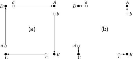
Figure 4: Two monotone assignments sending white points to black ones: (a) an assignment that is vastly non-optimal in terms of quadratic cost but cannot be improved by any pair interchange; (b) the optimal assignment, shown for comparison.

Actually, a much stronger condition, called cyclic monotonicity, is needed in order to minimize the cost. It requires $k$-monotonicity for any $k$ between $2$ and $N$; the latter is defined by taking any $k$ Eulerian positions with their corresponding Lagrangian antecedents and requiring that the cost (34) should not decrease under an arbitrary reassignment of the Lagrangian positions within the set of Eulerian positions taken. Note that the usual monotonicity corresponds to 2-monotonicity (stability with respect to pair exchanges).

A strategy called PIZA (Path Interchange Zel’dovich Approximation) for constructing monotone correspondences between Lagrangian and Eulerian positions has been proposed by Croft & Gaztañaga (1997). In PIZA, a randomly chosen tentative correspondence between initial and final positions is successively improved by swapping randomly selected pairs of initial particles whenever (36) is not satisfied. After the cost (34) ceases to decrease between iterations, an approximation to a monotone correspondence is established, which is generally neither unique, as already observed by Valentine, Saunders & Taylor (2000) in testing PIZA reconstruction, nor optimal. We shall come back to this in Sections 5 and 7.3.

4.2 Nuts and bolts of solving the assignment problem

For a general set of $N$ unit masses, the assignment problem with the cost function (34) has a single solution which can obviously be found by examining all $N!$ permutations. However, unlike computationally hard problems, such as the travelling salesman’s, the assignment problem can be handled in ‘polynomial time’ – actually in not more than $O(N^{3})$ operations. All methods achieving this use a so-called dual formulation of the problem, based on a relaxation similar to that applied by Kantorovich to the optimal mass transportation (Section 3.3; a brief introduction to duality is given in Appendix C.2). In this section we explain the basics of this technique, using a variant of a simple mechanical model introduced in a more general setting by Hénon (1995, 2002).

Consider the general assignment problem of minimizing the cost (35) over all permutations $j(i)$. We replace it by a ‘relaxed,’ linear programming problem of minimizing

$$\tilde{I}=\sum_{i,j=1}^{N}c_{ij}f_{ij},$$ (37)

where auxiliary variables $f_{ij}$ satisfy

$$f_{ij}\geq 0,\qquad\sum_{k=1}^{N}f_{kj}=\sum_{k=1}^{N}f_{ik}=1$$ (38)

for all $i$, $j$, an obvious discrete analogue of (31). We show now that it is possible to build a simple mechanical device (Fig. 5) which solves this relaxed problem and that the solution will in fact determine a minimizing permutation in the original assignment problem (i.e., for any $i$ or $j$ fixed, only one $f_{ij}$ will be unit and all other zero). The device acts as an analogue computer: the numbers involved in the problem are represented by physical quantities, and the equations are replaced by physical laws.

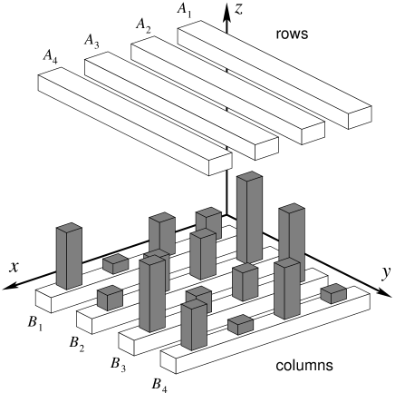
Figure 5: An analogue computer solving the assignment problem for $N=4$.

Define coordinate axes $x$, $y$, $z$ in space, with the $z$ axis vertical. We take two systems of $N$ horizontal rods, parallel to the $x$ and $y$ axes respectively, and call them columns and rows, referring to columns and rows of the cost matrix. Each rod is constrained to move in a corresponding vertical plane while preserving the horizontal orientation in space. For a row rod $A_{i}$, we denote the $z$ coordinate of its bottom face by $\alpha_{i}$ and for a column rod $B_{j}$, we denote the $z$ coordinate of its top face $\beta_{j}$. Row rods are placed above column rods, therefore $\alpha_{i}\geq\beta_{j}$ for all $i,j$ (see Fig. 5).

Upper (row) rods are assumed to have unit weight, and lower (column) rods to have negative unit weight, or unit ‘buoyancy.’ Therefore both groups of rods are subject to gravitational forces pulling them together. However, this movement is obstructed by $N^{2}$ small vertical studs of negligible weight put on column rods just below row rods. A stud placed at projected intersection of column $B_{j}$ and row $A_{i}$ has length $C-c_{ij}$ with a suitably large positive constant $C$ and thus constrains the quantities $\alpha_{i}$ and $\beta_{j}$ to satisfy the stronger inequality

$$\alpha_{i}-\beta_{j}\geq C-c_{ij}.$$ (39)

The potential energy of the system is, up to a constant,

$$U=\sum_{i=1}^{N}\alpha_{i}-\sum_{j=1}^{N}\beta_{j}.$$ (40)

In linear programming, the problem of minimizing (40) under the set of constraints given by (39) is called the dual problem to the ‘relaxed’ one (37)–(38) (see Appendix C.2); the $\alpha$ and $\beta$ variables are called the dual variables.

The analogue computer does in fact solve the dual problem. Indeed, first hold the two groups of rods separated from each other and then release them, so that the system starts to evolve. Rows will go down, columns will come up, and contacts will be made with the studs. Aggregates of rows and columns will be progressively formed and modified as new contacts are made, giving rise to a complex evolution. Eventually the system reaches an equilibrium, in which its potential energy (40) is minimum and all constraints (39) are satisfied (Hénon, 2002). Moreover, it may be shown that the solution to the original problem (37)–(38) is expressible in terms of the forces exerted by the rods on each other at equilibrium and is typically a one-to-one correspondence between the $A_{i}$s and the $B_{j}$s (for details, see Appendix C.3).

The common feature of many existing algorithms for solving the assignment problem, which makes them more effective computationally than the simple enumeration of all $N!$ permutations, is the use of the intrinsically continuous, geometric formulation in terms of the pair of linear programming problems (37)–(38) and (40)–(39). The mechanical device provides a concrete model for this formulation; in fact, assignment algorithms can be regarded as descriptions of specific procedures to make the machine reach its equilibrium state. An introduction into algorithmic aspects of solving the assignment problem, including a proof of the $O(N^{3})$ theoretical bound on the number of operations, based on the Hungarian method of Kuhn (1955), may be found in Papadimitriou & Steiglitz (1982).

In spite of the general $O(N^{3})$ theoretical bound, various algorithms may show very different performance when applied to a specific optimization problem. During the preparation of the earlier publication (Frisch et al., 2002) the dual simplex method of Balinski (1986) was used, with some modifications inspired by algorithm B of Hénon (2002). Several other algorithms were tried subsequently, including an adaptation of algorithm A of the latter reference and the algorithm of Burkard & Derigs (1980), itself based on the earlier work of Tomizawa (1971). For the time being, the fastest running code by far is based on the auction algorithm of Bertsekas (1992, 2001), arguably the most effective of existing ones, which is discussed in the next section. Needless to say, all these algorithms arrive at the same solution to the assignment problem with given data but can differ by several orders of magnitude in the time it takes to complete the computation.

4.3 The auction algorithm

We explain here the essense of the auction algorithm in terms of our mechanical device. Note that the original presentation of this algorithm (Bertsekas, 1981, 1992, 2001) is based on a different perspective, that of an auction, in which the optimal assignment appears as an economic rather than a mechanical equilibrium; the interested reader will benefit much from reading these papers.

Put initially the column rods at zero height and all row rods well above them, so that no contacts are made and constraints (39) are satisfied. To decrease the potential energy, let now the row rods descend while keeping the column rods fixed. Eventually all row rods will meet studs placed on column rods and stop. Some column rods may then come in contact with multiple row rods. Such rods are overloaded: if they were not prevented from moving they would descend.

Note that at this stage any column rod $A_{i}$ has established a contact with a row rod $B_{j}$ for which the stud length $C-c_{ij}$ is the maximum and the cost $c_{ij}$ the minimum among other $B$s; for $c_{ij}=|{\mn@boldsymbol{x}}_{i}-{\mn@boldsymbol{q}}_{j}|^{2}/2$, this means that any Eulerian position ${\mn@boldsymbol{x}}_{i}$ is coupled to its nearest Lagrangian neighbour ${\mn@boldsymbol{q}}_{j}$. This coupling is a reasonable guess for the optimal assignment; should it happen to be one-to-one, then the equilibrium, and with it the optimal assignment, would be reached. It is usually not, so there are overloaded $B$ rods and the following procedure is applied to find a compromise between minimization of the total cost and the requirement of one-to-one correspondence.

Take any overloaded rod $B_{j}$ and let it descend while keeping other column rods fixed. As $B_{j}$ descends, row rods touching it will follow its motion until they meet studs of other column rods and stay behind. The downward motion of $B_{j}$ is stopped only when the last row rod touching $B_{j}$ is about to lose its contact. We then turn to any other overloaded column rod and repeat the procedure as often as needed.

This general step can be viewed as an auction in which row rods bid for the descending column rod, offering prices equal to decreases in their potential energy as they follow its way down. As the column rod descends, thereby increasing its price, the auction is won by the row rod able to offer the largest bidding increment, i.e., to decrease its potential energy by the largest amount while not violating the constraints posed by studs of the rest of column rods. For computational purposes it suffices to compute bidding increments for all competing row rods from the dual $\alpha$ and $\beta$ variables and assign the descending column rod $B_{j}$ to the highest bidder $A_{i}$, decreasing their heights $\beta_{j}$ and $\alpha_{i}$ correspondingly.

Observe that, at each step, the total potential energy $U$ defined by (40) decreases by the largest amount that can be achieved by moving the descending column rod without violating the constraints. Since (40) is obviously nonnegative, the descent cannot proceed indefinitely, and the process may be expected to converge quite fast to a one-to-one pairing that solves the assignment problem.

However, as observed by Bertsekas (1981, 1992, 2001), this ‘naive’ auction algorithm may end up in an infinite cycle if several row rods bid for a few equally favourable column rods, having thus zero bidding increments. To break such cycles and also to accelerate convergence, a perturbation mechanism is introduced in the algorithm. Namely, the constraints (39) are replaced by weaker ones

$$\alpha_{i}-\beta_{j}\geq C-c_{ij}-\epsilon$$ (41)

for a small positive quantity $\epsilon$, and in each auction the descending column rod is pushed down by $\epsilon$ in addition to decreasing its height by the bidding increment. It can be shown that this reformulated process terminates in a finite number or rounds; moreover, if all stud lengths are integer and $\epsilon$ is smaller than $1/N$, then the algorithm terminates at an assignment that is optimal in the unperturbed problem (Bertsekas, 1992).

The third ingredient in the Bertsekas algorithm is the idea of $\epsilon$-scaling. When the values of dual variables are already close to the solution of the dual problem, it usually takes relatively few rounds of auction to converge to a solution. Thus one can start with large $\epsilon$ to compute a rough approximation for dual variables fast, without worrying about the quality of the assignment, and then proceed reducing $\epsilon$ in geometric progression until it passes the $1/N$ threshold, assuring that the assignment thus achieved solves the initial problem.

Bertsekas’ algorithm is especially fast for sparse assignment problems, in which rods $A_{i}$ and $B_{j}$ can be matched only if the pair $(i,j)$ belongs to a given subset $\mathcal{A}$ of the set of $N^{2}$ possible pairs. We call such pairs valid and define the filling factor to be the proportion of valid pairs $f=|\mathcal{A}|/N^{2}$. When this factor is small, computation can be considerably faster: to find the bidding increment for a rod $A_{i}$, we need only to run over the list of rods $B_{j}$ such that $(i,j)$ is a valid pair.

Note also that the decentralized structure of the algorithm facilitates its parallelization (see references in Bertsekas, 1992, 2001).

4.4 The auction algorithm for the MAK reconstruction

We now describe the adaptation of the auction algorithm to the MAK reconstruction. Experiments with various programs contained in Bertsekas’ publicly available package (http://web.mit.edu/dimitrib/www/auction.txt) showed that the most effective for our problem is auction_flp. It assumes integer costs $c_{ij}$, which in our case requires proper scaling of the cost matrix. To achieve this, the unit of length is adjusted so that the size of the reconstruction patch equals 100, and then the square of the distance between an initial and a final position is rounded off to an integer. In our application, row and column rods correspond to Eulerian and Lagrangian positions, respectively. As the MAK reconstruction is planned for application to catalogues of $10^{5}$ and more galaxies, we do not store the cost matrix, which would require an $O(N^{2})$ storage space, but rather compute its elements on demand from the coordinates, which requires only $O(N)$ space.

Our problem is naturally adapted for a sparse description if galaxies travel only a short distance compared to the dimensions of the reconstruction patch. For instance, in the simulation discussed in Section 5, the r.m.s. distance traveled is only about $10\,h^{-1}$ Mpc, or 5% of the size of the simulation box, and the largest distance traveled is about 15% of this size. So we may assume that in the optimal assignment distances between paired positions will be limited. We define then a critical distance $d_{\rm crit}$ and specify that a final position ${\mn@boldsymbol{x}}_{i}$ and an initial position ${\mn@boldsymbol{q}}_{j}$ form a valid pair only if they are within less than $d_{\rm crit}$ from each other. This critical distance must be adjusted carefully: if it is too small, we risk excluding the optimal assignment; if it is taken too large, the benefit of the sparse description is lost.

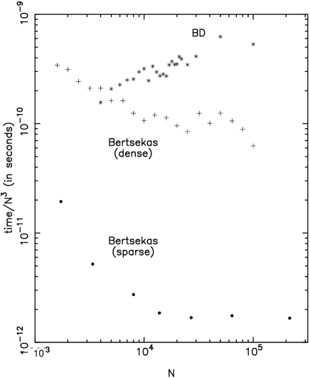
Figure 6: Computing time for different algorithms as a function of the number $N$ of points (divided by $N^{3}$ for normalization). Asterisks, the Burkard & Derigs (1980) algorithm (BD); crosses and points, the dense and sparse versions of the auction algorithm (described in the text).

However, the saving in computing time achieved by sparse description has to be paid for in storage space: to store the set $\mathcal{A}$ of valid pairs, storage of size $|\mathcal{A}|=fN^{2}$ is needed, which takes us back to the $O(N^{2})$ storage requirement. We have explored two solutions to this problem.

1. Use a dense description nevertheless, i.e. the one where all pairs $(i,j)$ are valid and there is no need to store the set $A$. The auction program is easily adapted to this case (in fact this simplifies the code). However, we forfeit the saving in time provided by the sparse structure.

2. The sparse description can be preserved if the set of valid pairs is computed on demand rather than stored. This is easy if initial positions fill a uniform cubic grid, the simplest discrete approximation to the initial quasi-uniform distribution of matter in the reconstruction problem. Thus, for a given final position ${\mn@boldsymbol{x}}_{i}$, the valid pairs correspond to points of the cubic lattice that lie inside a sphere of radius $d_{\rm crit}$ centered at ${\mn@boldsymbol{x}}_{i}$, so their list can be generated at run time.

Fig. 6 gives the computing time as a function of the number of points $N$ used in the assignment problem. Shown are the dense and sparse versions of the auction algorithm (in the latter, the critical distance squared was taken equal to 200) and the Burkard & Derigs (1980) algorithm, which ranked the next fastest in our experiments. The $N$ initial and final positions are chosen from the file generated by an $N$-body simulation described in Section 5; the choice is random except for the sparse algorithm, in which the initial positions are required to fill a cubic lattice. Hence, the performance of the sparse auction algorithm shown in the figure is not completely comparable to that of the two other algorithms.

It is evident that the difference in computing time between the dense auction and the Burkard & Derigs algorithms steadily increases. In the vicinity of $N=10^{5}$, the dense auction algorithm is about 10 times faster than the other one. For the sparse version, the decrease in computing time is spectacular: as could be expected, the ratio of computing times for the two versions of the auction algorithm is of the order of $f$. For large $N$, the $O(N^{3})$ asymptotic of the computing time is quite clear for the sparse auction algorithm. For two other algorithms, similar asymptotic was found for larger $N$ in other experiments (not shown).

In all three cases shown, the initial positions fill a constant volume while $N$ is varied. This is what we call constant-volume computations. In the sparse case, this results in a constant filling factor, equal to the ratio of the volume of the sphere with radius $d_{\mathrm{crit}}$ to the volume occupied by the initial positions. Here this filling factor is about $f=0.019$. Another choice, not shown in the figure, is that of constant-density computations, when the initial positions are taken from a volume whose size increases with $N$. In this case the time dependence of algorithms for large $N$ is of the order of $N^{1.5}$.

We finally observe that the sparse auction algorithm applied to the MAK reconstruction requires 5 hours of single-processor CPU time on a 667 MHz COMPAQ/DEC Alpha machine for 216,000 points.

5 Testing the MAK reconstruction

In this section we present results of our testing the MAK reconstruction against data of cosmological $N$-body simulations. In a typical simulation of this kind, the dark matter distribution is approximated by $N$ particles of identical mass. Initially the particles are put on a uniform cubic grid and given velocities that form a realization of the primordial velocity field whose statistics is prescribed by a certain cosmological model. Trajectories of particles are then computed according to the Newtonian dynamics in a comoving frame, using periodic boundary conditions. The reconstruction problem is therefore to recover the pairing between the initial (Lagrangian) positions of the particles and their present (Eulerian) positions in the $N$-body simulation, knowing only the set of computed Eulerian positions in the physical space.

We test our reconstruction against a simulation of $128^{3}$ particles in a box of $200\,h^{-1}$ Mpc size (where $h$ is the Hubble parameter in units of 100 km  s^-1 Mpc^-1) performed using the adaptive P³M code HYDRA (Couchman, Thomas & Pearce, 1995). A $\Lambda$CDM cosmological model is used with parameters $\Omega_{m}=0.3$, $\Omega_{\Lambda}=0.7$, $h=0.65$, $\sigma_{8}=0.9$. The value of these parameters within the model are determined by fitting the observed cosmic microwave background (CMB) spectrum. The output of the $N$-body simulation is illustrated in Fig. 7 by a projection onto the $x$-$y$ plane of a 10% slice of the simulation box.

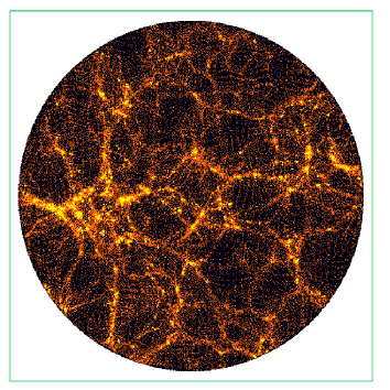
Figure 7: $N$-body simulation output in the Eulerian space used for testing our reconstruction method (shown is a projection onto the $x$-$y$ plane of a 10% slice of the simulation box of size $200h^{-1}$ Mpc). Points are highlighted in yellow when reconstruction fails by more than $6.25\,h^{-1}$ Mpc, which happens mostly in high-density regions.

Since the simulation assumes periodic boundary conditions, some Eulerian positions situated near boundaries may have their Lagrangian antecedents at the opposite side of the simulation box. Suppressing the resulting spurious large displacements is crucial for successful reconstruction. Indeed, for a typical particle displacement of 1/20 the box size, spurious box-wide leaps of 1% of the particles will generate a contribution to the quadratic cost (34) four times larger than that of the rest. To suppress such leaps, for each Eulerian position that has its antecedent Lagrangian position at the other side of the simulation box, we add or subtract the box size from coordinates of the latter (in other words, we are considering the distance on a torus). In what follows we refer to this procedure as the periodicity correction.

We first present reconstructions for three samples of particles initially situated on Lagrangian subgrids with meshes given by $\Delta x=6.25\,h^{-1}$ Mpc, $\Delta x/2$ and $\Delta x/4$. To further reduce possible effects of the unphysical periodic boundary condition, we truncate the data by discarding those points whose Eulerian positions are not within the sphere of radius $16\Delta x$ placed at the centre of the simulation box (for the largest $\Delta x$ its diameter coincides with the box size). The problem is then confined to finding the pairing between the remaining Eulerian positions and the set of their periodicity-corrected Lagrangian antecedents in the $N$-body simulation.

The results are shown in Figs. 8–11. The main plots show the scatter of reconstructed vs. simulation Lagrangian positions for the same Eulerian positions. For these diagrams we introduce a ‘quasi-periodic projection’

$$\tilde{q}\equiv(q_{1}+\sqrt{2}q_{2}+\sqrt{3}q_{3})/(1+\sqrt{2}+\sqrt{3})$$ (42)

of the vector ${\mn@boldsymbol{q}}$, which ensures a one-to-one correspondence between $\tilde{q}$-values and points on the regular Lagrangian grid. The insets are histograms (by percentage) of distances, in reconstruction mesh units, between the reconstructed and simulation Lagrangian positions; the first darker bin, slightly less than one mesh in width, corresponds to perfect reconstruction (thereby allowing a good determination of the peculiar velocities of galaxies).

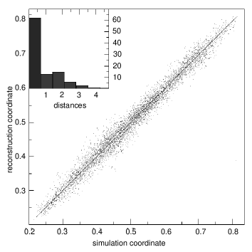
Figure 8: Test of the MAK reconstruction for a sample of $N^{\prime}=17,178$ points initially situated on a cubic grid with mesh $\Delta x=6.25\,h^{-1}$ Mpc. The scatter diagram plots true versus reconstructed initial positions using a quasi-periodic projection which ensures one-to-one correspondence with points on the cubic grid. The histogram inset gives the distribution (in percentages) of distances between true and reconstructed initial positions; the horizontal unit is the sample mesh. The width of the first bin is less than unity to ensure that only exactly reconstructed points fall in it. Note that more than sixty percent of the points are exactly reconstructed.

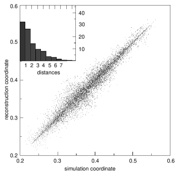
Figure 9: Same as Fig. 8 but with $N^{\prime}=19,187$ and a sample mesh of $\Delta x/2=3.125\,h^{-1}$ Mpc. Exact reconstruction is down to 35%.

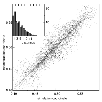
Figure 10: Same as Fig. 8 but with $N^{\prime}=23,111$ and a sample mesh of $\Delta x/4=1.56\,h^{-1}$ Mpc. Exact reconstruction is down to 14%.

With the mesh size $\Delta x$, Lagrangian positions of 62% of the sample of 17,178 points are reconstructed perfectly and about 75% are placed within not more than one mesh. With the $\Delta x/2$ grid, we still have 35% of exact reconstruction out of 19,187 points, but only 14% for the $\Delta x/4$ grid with 23,111 points.

We also performed a reconstruction on a random sample of 100,000 Eulerian positions taken with their periodicity-corrected Lagrangian antecedents out of the whole set of $128^{3}$ particles, without any restrictions. This reconstruction, with the effective mesh size (average distance between neighbouring points) of 4.35$h^{-1}$Mpc, gives 51% of perfect reconstruction (Fig. 11).

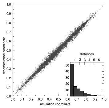
Figure 11: Same as Fig. 8 with $N^{\prime}=10^{5}$ points selected at random, neighbouring points being typically $4.35\,h^{-1}$ Mpc apart. Exact reconstruction is in excess of 50%.

We compared these results with those of the PIZA reconstruction method (see Section 4.1 and Croft & Gaztañaga, 1997), which gives a 2-monotone but not necessarily optimal pairing between Lagrangian and Eulerian positions. We applied the PIZA method on the $\Delta x$ grid and obtained typically 30–40% exactly reconstructed positions, but severe non-uniqueness: for two different seeds of the random generator used to set up the initial tentative assignment, only about half of the exactly reconstructed positions were the same (see figs. 3 and 7 of Mohayaee et al. (2003) for an illustration). We also implemented a modification of the PIZA method establishing 3-monotonicity (monotonicity with respect to interchanges of 3 points instead of pairs) and checked that it does not give a significant improvement over the original PIZA.

In comoving coordinates, the typical displacement of a mass element is about 1/20 the box size, that is about $10\,h^{-1}$ Mpc. This is not much larger than the coarsest grid of $6.25\,h^{-1}$ Mpc used in testing MAK which gave 62% of exact reconstruction. Nevertheless there are 18 other grid points within $10\,h^{-1}$ Mpc of any given grid point, so that this high percentage cannot be trivially explained by the smallness of the displacement. Note that without the periodicity correction, the percentage of exact reconstruction for the coarsest grid degraded significantly (from 62% to 45%) and the resulting cost was far from the true minimum.

For real catalogues, reconstruction has to be performed for galaxies whose positions are specified in the redshift space, where they appear to be displaced radially (along the line of sight) by an amount proportional to the radial component of the peculiar velocity. Thus, at the present epoch, the redshift position ${\mn@boldsymbol{s}}$ of a mass element situated at the point ${\mn@boldsymbol{x}}$ in the physical space is given by

$${\mn@boldsymbol{s}}={\mn@boldsymbol{x}}+\hat{\mn@boldsymbol{x}}\beta\left({\mn@boldsymbol{v}}\cdot\hat{\mn@boldsymbol{x}}\right),$$ (43)

where ${\mn@boldsymbol{v}}$ is the peculiar velocity in the comoving coordinates ${\mn@boldsymbol{x}}$ and the linear growth factor time $\tau$, $\hat{\mn@boldsymbol{x}}$ denotes the unit normal in the direction of ${\mn@boldsymbol{x}}$, and the parameter $\beta$ equals $0.486$ in our $\Lambda$CDM model.

Following Valentine et al. 2000; Monaco & Efstathiou, 1999, see also, we use the Zel’dovich approximation (ZA) to render our MAK quadratric cost function in the ${\mn@boldsymbol{s}}$ variable. As follows from (3.1), in this approximation the peculiar velocity is given by

$${\mn@boldsymbol{v}}=\frac{1}{\tau}({\mn@boldsymbol{x}}-{\mn@boldsymbol{q}}).$$ (44)

At the present time, since $\tau_{0}=1$, this together with (43) gives

$$({\mn@boldsymbol{s}}-{\mn@boldsymbol{q}})\cdot\hat{\mn@boldsymbol{x}} = (1+\beta)({\mn@boldsymbol{x}}-{\mn@boldsymbol{q}})\cdot\hat{\mn@boldsymbol{x}},$$ (45)

$$|{\mn@boldsymbol{s}}-{\mn@boldsymbol{q}}|^{2} = |{\mn@boldsymbol{x}}-{\mn@boldsymbol{q}}|^{2}+\beta(\beta+2)\bigl{(}({\mn@boldsymbol{x}}-{\mn@boldsymbol{q}})\cdot\hat{\mn@boldsymbol{x}}\bigr{)}^{2}.$$ (46)

Combining now these two equations and using the fact that, by (43), the vectors ${\mn@boldsymbol{x}}$ and ${\mn@boldsymbol{s}}$ are collinear and therefore $\hat{\mn@boldsymbol{x}}=\pm\hat{\mn@boldsymbol{s}}$, we may write the quadratic cost function as

$$\frac{1}{2}|{\mn@boldsymbol{x}}-{\mn@boldsymbol{q}}|^{2}=\frac{1}{2}|{\mn@boldsymbol{s}}-{\mn@boldsymbol{q}}|^{2}-\frac{\beta(\beta+2)}{2(\beta+1)^{2}}\bigl{(}({\mn@boldsymbol{s}}-{\mn@boldsymbol{q}})\cdot\hat{\mn@boldsymbol{s}}\bigr{)}^{2}.$$ (47)

The redshift-space reconstruction is then in principle reduced to the physical-space reconstruction. Note however that the redshift transformation of Eulerian positions may fail to be one-to-one if the peculiar component of velocity field in the proper space coordinates exceeds the Hubble expansion component. This undermines the simple reduction outlined above for catalogues confined to small distances.

We have performed a MAK reconstruction with the redshift-modified cost function (47). The redshift positions were computed for the simulation data with peculiar velocities smoothed over a sphere with radius of 1/100 the box size ($2\,h^{-1}$ Mpc). This reconstruction led to 43% of exactly reconstructed positions and 60% which are within not more than one $\Delta x$ mesh from their correct positions (see Fig. 12; a scatter diagram is omitted because it is quite similar to that in Fig. 8). A comparison of the redshift-space MAK reconstruction with the physical-space MAK reconstruction shows that almost 50% of exactly reconstructed positions correspond to the same points. This test shows that the MAK method is robust with respect to systematic errors introduced by the redshift transformation.

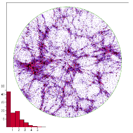
Figure 12: Test of the redshift-space variant of the MAK reconstruction based on the same data as Fig. 8. The circular redshift map (violet points) corresponds to the same physical-space slice as displayed in Fig. 7 (the observer is taken at the center of the simulation box). Points are highlighted in red when reconstruction fails by more than one mesh.

Our results demonstrate the essentially potential character of the Lagrangian map above $\sim 6\,h^{-1}$ Mpc (within the $\Lambda$CDM model) and perhaps at somewhat smaller scales.

Although it is not our intention in this paper to actually implement the MAK reconstruction on real catalogues, a few remarks are in order. The effect of the catalogue selection function can be handled by standard techniques; for instance one can assign each galaxy a ‘mass’ inversely proportional to the catalog selection function (Nusser & Branchini, 2000; Valentine et al., 2000; Branchini et al., 2002). Biasing can be taken into account in a similar manner (Nusser & Branchini, 2000). Both these modifications and the natural scatter of masses in the observational catalogues require that massive objects be represented by clusters of multiple Eulerian points of unit mass (with the correspondingly increased number of points on a finer grid in the Lagrangian space), which reduces the problem to a variant of the usual assignment. We also observe that real catalogues involve truncation, that is data available only over a finite region. As already discussed in Section 3.4, this is not a serious problem provided a sufficiently large patch is available. Actually, as noted earlier in this Section, the data used in testing have been truncated spherically, without significantly affecting the quality of the reconstruction.

In the redshift-space modification, more accurate determination of peculiar velocities can be done using second-order Lagrangian perturbation theory. Note also that, for the observational catalogues, the motion of the local group itself should also be accounted for (Taylor & Valentine, 1999).

6 Reconstruction of the full self-gravitating dynamics

The MAK reconstruction discussed in Sections 3 and 4 was performed under the assumption of a potential Lagrangian map and of the absence of multi-streaming. The tests done in Section 5 indicate that potentiality works well at scales above $6\,h^{-1}$ Mpc, whereas multi-streaming is mostly believed to be unimportant above a few megaparsecs. There could thus remain a substantial range of scales over which the quality of the reconstruction can be improved by relaxing the potentiality assumption and using the full self-gravitating dynamics. Here we show that, as long as the dynamics can be described by a solution to the Euler–Poisson equations, the prescription of the present density field still determines a unique solution to the full reconstruction problem. We give only the main ideas, technical details being left for Appendix D (a mathematically rigorous proof may be found in Loeper (2003)). In order to make the exposition self-contained, we also give in Appendix C an elementary introduction to convexity and duality which are used for the derivation (and also elsewhere in this paper).

We shall start from an Eulerian variational formulation of the Euler–Poisson equations in an Einstein–de Sitter universe, which is an adaptation of a variational principle given by Giavalisco et al. (1993). We minimize the action

$$I=\frac{1}{2}\int_{0}^{\tau_{0}}\mathrm{d}\tau\int\mathrm{d}^{3}{\mn@boldsymbol{x}}\,\tau^{3/2}\left(\rho|{\mn@boldsymbol{v}}|^{2}+\frac{3}{2}|{\nabla_{{\mn@boldsymbol{x}}}}\varphi_{\mathrm{g}}|^{2}\right),$$ (48)

under the following four constraints: the Poisson equation (3), the mass conservation equation (2) and the boundary conditions that the density field be unity at $\tau=0$ and prescribed at the present time $\tau=\tau_{0}$. The constraints can be handled by the standard method of Lagrange multipliers (here functions of space and time), which allows to vary independently the fields $\rho$, $\varphi_{\mathrm{g}}$ and ${\mn@boldsymbol{v}}$. The vanishing of the variation in ${\mn@boldsymbol{v}}$ gives ${\mn@boldsymbol{v}}=\tau^{-3/2}{\nabla_{{\mn@boldsymbol{x}}}}\theta$, where $\theta({\mn@boldsymbol{x}},\tau)$ is the Lagrange multiplier for the mass conservation constraint. Hence, the velocity is curl-free. The vanishing of the variation in $\rho$ gives then

$${\partial_{\tau}}\theta+\frac{1}{2\tau^{3/2}}|{\nabla_{{\mn@boldsymbol{x}}}}\theta|^{2}+\frac{3}{2\tau}\psi=0.$$ (49)

By taking the gradient, this equation goes over into the momentum equation (1), repeated here for convenience:

$${\partial_{\tau}}{\mn@boldsymbol{v}}+({\mn@boldsymbol{v}}\cdot{\nabla_{{\mn@boldsymbol{x}}}}){\mn@boldsymbol{v}}=-\frac{3}{2\tau}({\mn@boldsymbol{v}}+{\nabla_{{\mn@boldsymbol{x}}}}\varphi_{\mathrm{g}}).$$ (50)

It is noteworthy that, if in the action we replace $3/2$ both in the exponent of $\tau$ and in the gravitational energy term by $3\alpha/2$, we obtain (50) but also with a $3\alpha/(2\tau)$ factor in the right-hand side. The Zel’dovich approximation and the associated MAK reconstruction amount clearly to setting $\alpha=0$, so as to recover the ‘free-streaming action’

$$I=\frac{1}{2}\int_{0}^{\tau_{0}}\mathrm{d}\tau\int\mathrm{d}^{3}{\mn@boldsymbol{x}}\;\rho|{\mn@boldsymbol{v}}|^{2},$$ (51)

whose minimization is easily shown to be equivalent to that of the quadratic cost function (23).

Assuming the action (48) to be finite, existence of a minimum is mostly a consequence of the action being manifestedly non-negative. Here it is interesting to observe that the Lagrangian, which is the difference between the kinetic energy and the potential energy, is positive whereas the Hamiltonian which is their sum does not have a definite sign. As a consequence, our two-point boundary problem is, as we shall see, well posed but the initial-value problem for the Euler–Poisson system is not well posed since formation of caustics after a finite time cannot be ruled out.

Does the variational formulation imply uniqueness of the solution? This would be the case if the action were a strictly convex functional (see Appendix C.1), which is guaranteed to have one and only one minimum. The action as written in (48) is not convex in the $\rho$ and ${\mn@boldsymbol{v}}$ variables, but can be rendered so by introducing the mass flux ${\mn@boldsymbol{J}}=\rho\,{\mn@boldsymbol{v}}$; the kinetic energy term becomes then $|{\mn@boldsymbol{J}}|^{2}/(2\rho)$, which is convex in the ${\mn@boldsymbol{J}}$ and $\rho$ variables.

Strict convexity is particularly cumbersome to establish, but there is an alternative way, known as duality: by a Legendre-like transformation the variational problem is carried into a dual problem written in terms of dual variables; the minimum value for the original problem is the maximum for the dual problem. It turns out that the difference of these equal values can be rewritten as a sum of non-negative terms, each of which must thus vanish. This is then used to prove (i) that the difference between any two solutions to the variational problem vanishes and (ii) that any curl-free solution to the Euler–Poisson equations with the prescribed boundary conditions for the density also minimizes the action. All this together establishes uniqueness. For details see Appendix D.

Several of the issues raised in connection with the MAK reconstruction appear in almost the same form for the Euler–Poisson reconstruction. First, we are faced again with the problem that, when reconstructing from a finite patch of the present universe, we need either to know the shape of the initial domain or to make some hypothesis as to the present distribution of matter outside this patch. Second, just as for the MAK reconstruction, the proof of uniqueness still holds when the present density $\rho_{0}({\mn@boldsymbol{x}})$ has a singular part, that is, when some matter is concentrated. Again, we shall have full information on the initial shape of collapsed regions but not on the initial fluctuations inside them. The particular solution obtained from the variational formulation is the only solution which stays smooth for all times prior to $\tau_{0}$.

We also note that, at this moment and probably for quite some time, 3D catalogues sufficiently dense to allow reconstruction will be limited to fairly small redshifts. Eventually, it will however become of interest to perform reconstruction ‘along our past light-cone’ with data not all at $\tau_{0}$. The variational approach can in principle be adapted to handle such reconstruction.

In previous sections we have seen how to implement reconstruction using MAK, which is equivalent to using the simplified action (51). Implementation using the full Euler–Poisson action (48) is mostly beyond the scope of this paper, but we shall indicate some possible directions. In principle it should be possible to adapt to the Euler–Poisson reconstruction the method of the augmented Lagrangian which has been applied to the two-dimensional Monge–Ampère equation (Benamou & Brenier, 2000). An alternative strategy, which allows reduction to MAK-type problems, uses the idea of ‘kicked burgulence’ (Bec, Frisch & Khanin, 2000) in which, in order to solve the one or multi-dimensional Burgers equation

$${\partial_{\tau}}{\mn@boldsymbol{v}}+({\mn@boldsymbol{v}}\cdot{\nabla_{{\mn@boldsymbol{x}}}}){\mn@boldsymbol{v}}=\mn@boldsymbol{f}({\mn@boldsymbol{x}},\tau),\quad{\mn@boldsymbol{v}}=-{\nabla_{{\mn@boldsymbol{x}}}}\varphi_{\mathrm{v}},$$ (52)

one approximates the force by a sum of delta-functions in time:

$$\mn@boldsymbol{f}({\mn@boldsymbol{x}},\tau)\approx\sum_{i}\delta(\tau-\tau_{i})\mn@boldsymbol{g}_{i}({\mn@boldsymbol{x}}).$$ (53)

In the present case, the $\mn@boldsymbol{g}_{i}({\mn@boldsymbol{x}})$ are proportional to the right-hand side of (50) evaluated at the kicking times $\tau_{i}$. The action becomes then a sum of free-streaming Zel’dovich-type actions plus discrete gravitational contributions stemming from the kicking times. Between kicks one can use our MAK solution. At kicking times the velocity undergoes a discontinuous change which is related to the gravitational potential (and thus to the density) at those times. The densities at kicking times can be determined by an iterative procedure. The kicking strategy also allows to do redshift-space reconstruction by applying the redshift-space modified cost (Section 5) at the last kick.

7 Comparison with other reconstruction methods

Reconstruction started with Peebles’ (1989) work, in which he compared reconstructed and measured peculiar velocities for a small number of Local Group galaxies, situated within a few Mpc. The focus of reconstruction work has now moved to tackling the rapidly growing large 3D surveys (see, e.g. Frieman & Szalay, 2000). It is not our intention here to review all the work on reconstruction; rather we shall discuss how some of the previously used methods can be reinterpreted in the light of the optimization approach to reconstruction. For convenience we shall divide methods into perturbative (Section 7.1), probabilistic (Section 7.2), and variational (Section 7.3). Methods such as POTENT (Dekel et al., 1990), whose purpose is to obtain the full peculiar velocity field from its radial components using the (Eulerian) curl-free property, are not directly within our scope. Note that in its original Lagrangian form (Bertschinger & Dekel, 1989; Dekel et al., 1990) POTENT was assuming a curl-free velocity in Lagrangian coordinates, an assumption closely related to the potential assumption made for MAK, as already pointed out in Section 3.1. Even closer is the relation between MAK and the PIZA method of Croft & Gaztañaga (1997), discussed in Section 7.3, which is also based on minimization of quadratic action.

7.1 Perturbative methods

Nusser & Dekel (1992) have proposed using the Zel’dovich approximation backwards in time to obtain the initial velocity fluctuations and thus (by slaving) the density fluctuations. Schematically, their procedure involves two steps: (i) obtaining the present potential velocity field and (ii) integrating the Zel’dovich–Bernouilli equation back in time. Using the equality (in our notation) of the velocity and gravitational potentials, they point out that the velocity potential can be computed from the present density fluctuation field by solving the Poisson equation. This is a perturbative approximation to reconstruction in so far as it replaces the Monge–Ampère equation (19) by a linearized form. Indeed, when using the Zel’dovich approximation we have ${\mn@boldsymbol{q}}={\mn@boldsymbol{x}}-\tau{\mn@boldsymbol{v}}={\mn@boldsymbol{x}}+\tau{\nabla_{{\mn@boldsymbol{x}}}}\varphi_{\mathrm{v}}({\mn@boldsymbol{x}})$. We know that ${\mn@boldsymbol{q}}={\nabla_{{\mn@boldsymbol{x}}}}\Theta({\mn@boldsymbol{x}})$ with $\Theta$ satisfying the Monge–Ampère equation. The latter can thus be rewritten as

$$\det\left(\delta_{ij}+\tau\nabla_{x_{i}}\nabla_{x_{j}}\varphi_{\mathrm{v}}({\mn@boldsymbol{x}})\right)=\rho({\mn@boldsymbol{x}}),$$ (54)

where $\delta_{ij}$ denotes the identity matrix. If we now use the relation $\det(\delta_{ij}+\epsilon A_{ij})=1+\epsilon\sum_{i}A_{ii}+O(\epsilon^{2})$ and truncate the expansion at order $\epsilon$, we obtain the Poisson equation

$$\tau{\nabla^{2}_{{\mn@boldsymbol{x}}}}\varphi_{\mathrm{v}}({\mn@boldsymbol{x}})=\rho({\mn@boldsymbol{x}})-1=\delta({\mn@boldsymbol{x}}).$$ (55)

Of course, in one dimension no approximation is needed. From a physical point of view, equating the velocity and gravitational potentials at the present epoch amounts to using the Zel’dovich approximation in reverse and is actually inconsistent with the forward Zel’dovich approximation: the slaving which makes the two potentials equal initially does not hold in this approximation at later epochs. Replacing the Monge–Ampère equation by the Poisson equation is not consistent with a uniform initial distribution of matter and will in general lead to spurious multi-streaming in the initial distribution. Of course, if the present-epoch velocity field happens to be known one can try applying the Zel’dovich approximation in reverse. Nusser and Dekel observe that calculating the inverse Lagrangian map by ${\mn@boldsymbol{q}}={\mn@boldsymbol{x}}-\tau{\mn@boldsymbol{v}}$ does not work well (spurious multi-streaming appears) and instead integrate back in time the Zel’dovich–Bernouilli equation

$$\partial_{t}\varphi_{\mathrm{v}}={1\over 2}\left({\nabla_{{\mn@boldsymbol{x}}}}\varphi_{\mathrm{v}}\right)^{2},$$ (56)

which is obviously equivalent to the Burgers equation (13) with the viscosity $\nu=0$. One way of performing this reverse integration, which guarantees the absence of multi-streaming, is to use the Legendre transformation (18) to calculate $\Phi({\mn@boldsymbol{q}})$ from $\Theta({\mn@boldsymbol{x}})=|{\mn@boldsymbol{x}}|^{2}/2-\tau\varphi_{\mathrm{v}}({\mn@boldsymbol{x}})$ and then obtain the reconstructed initial velocity field as

$${\mn@boldsymbol{v}}_{\rm in}({\mn@boldsymbol{q}})={\mn@boldsymbol{v}}_{0}\left({\nabla_{{\mn@boldsymbol{q}}}}\Phi({\mn@boldsymbol{q}})\right).$$ (57)

This procedure can however lead to spurious shocks in the reconstructed initial conditions, due to inaccuracies in the present-epoch velocity data, unless the data are suitably smoothed. Finally, the improved reconstruction method of Gramann (1993) can be viewed as an approximation to the Monge–Ampère equation beyond the Poisson equation which captures part of the nonlinearity.

7.2 Probabilistic methods

Weinberg (1992) presents an original approach to reconstruction, which turns out to have hidden connections to optimal mass transportation. The key observations in his ‘Gaussianization’ technique are the following: (i) the initial density fluctuations are assumed to be Gaussian, (ii) the rank order of density values is hardly changed between initial and present states, (iii) the bulk displacement of large-scale features during dynamical evolution can be neglected. Assumption (i) is part of the standard cosmological paradigm. Assumption (iii) can of course be tested in $N$-body simulations. As we have seen in Section 5, a displacement of 10 $h^{-1}$Mpc is typical and can indeed be considered small compared to the size of the simulation boxes ($64\,h^{-1}$Mpc in Weinberg’s simulations and $200\,h^{-1}$Mpc in ours). Assumption (ii) means that the correspondence between initial and present values of the density $\rho$ (or of the contrast $\delta=\rho-1$) is monotone. This map, which can be determined from the empirical present data, can then be applied to all the data to produce a reconstructed initial density field. Finally, by running an $N$-body simulation initialized on the reconstructed field one can test the validity of the procedure, which turns out to be quite good and can be improved further by hybrid methods (Narayanan & Weinberg, 1998; Kolatt et al., 1996) combining Gaussianization with the perturbative approaches of Nusser & Dekel (1992) or Gramann (1993).

This technique is actually connected with mass transportation: starting with the work of Fréchet 1957a; 1957b; Rachev, 1984, see also, probabilists have been asking the following question: given two random variables $m_{1}$ and $m_{2}$ with two laws, say PDFs $p_{1}$ and $p_{2}$, can one find a joint distribution of $(m_{1},m_{2})$ with PDF $p_{12}(m_{1},m_{2})$ having the following properties: (i) $p_{1}$ and $p_{2}$ are the marginals, i.e. when $p_{12}$ is integrated over $m_{2}$ (respectively, $m_{1}$) one recovers $p_{1}$ (respectively, $p_{2}$), (ii) the correlation $\langle m_{1}m_{2}\rangle$ is maximum? Since $\langle m_{1}^{2}\rangle$ and $\langle m_{2}^{2}\rangle$ are obviously prescribed by the constraint that we know $p_{1}$ and $p_{2}$, maximizing the correlation is the same as minimizing the quadratic distance $\langle(m_{1}-m_{2})^{2}\rangle$. This is precisely an instance of the mass transportation problem with quadratic cost, as we defined it in Section 3.3. As we know, the optimal solution is obtained by a map from the space of $m_{1}$ values to that of $m_{2}$ values which is the gradient of a convex function. If $m_{1}$ and $m_{2}$ are scalar variables, the map is just monotone, as in the Gaussianization method (in the discrete setting this was already observed in Section 4.1). Hence Weinberg’s method may be viewed as requiring maximum correlation (or minimum quadratic distance in the above sense) between initial and present distributions of density fluctuations.

In principle the Gaussianization method can be extended to multipoint distributions, leading to a difficult multidimensional mass transportation problem which can be discretized into an assignment problem just as in Section 4.1. The contact of the maximum correlation assumption to the true dynamics is probably too flimsy to justify using such heavy machinery.

7.3 Variational methods

All variational approaches to reconstruction, starting with that of Peebles (1989), have common features: one uses a suitable Lagrangian and poses a two-point variational problem with boundary conditions prescribed at the present epoch by the observed density field, and at early times by requiring a quasi-uniform distribution of matter (more precisely, as we have seen in Section 2.1, by requiring that the solutions not be singular as $\tau\to 0$).

The Path Interchange Zel’dovich Approximation (PIZA) method of Croft & Gaztañaga (1997) and our MAK reconstruction techniques use a free-streaming Lagrangian in linear growth rate time. As we have seen in Section 3.1, this amounts to assuming adhesion dynamics. Once discretized for numerical purposes, the variational problem becomes an instance of the assignment problem. Croft & Gaztañaga (1997) have proposed a restricted procedure for solving it, which does not account for the Lagrangian potentiality and yields non-unique approximate solutions. As we have seen in Sections 4 and 5, the exact and unique solution can be found with reasonable CPU resources.

Turning now to the Peebles least action method, let us first describe it schematically, using our notation. In its original formulation it is applied to a discrete set of galaxies (assumed of course to trace mass) in an Einstein–de Sitter universe. The action, in our notation, can be written as

$$I = \displaystyle\int_{0}^{\tau_{0}}\mathrm{d}\tau\,\frac{3}{2\tau^{1/2}}\left(\sum_{i}\frac{m_{i}\tau^{2}}{3}\left|\frac{d{\mn@boldsymbol{x}}_{i}}{d\tau}\right|^{2}\right.$$ (58)

$$\displaystyle\left.+\frac{3G}{2}\sum_{i\neq j}\frac{m_{i}m_{j}}{|{\mn@boldsymbol{x}}_{i}-{\mn@boldsymbol{x}}_{j}|}+\pi G\bar{\varrho}_{0}\sum_{i}m_{i}|{\mn@boldsymbol{x}}_{i}|^{2}\right),$$

where $m_{i}$ is the mass and ${\mn@boldsymbol{x}}_{i}$ the comoving coordinate of $i$th galaxy (see also Nusser & Branchini, 2000). This is supplemented by the boundary condition that the present positions of the galaxies are known and that the early-time velocities satisfy

$$\tau^{3/2}\frac{d{\mn@boldsymbol{x}}_{i}}{d\tau}\to 0\qquad{\rm for}\,\,\,\,\tau\to 0.$$ (59)

This particle approach was extended by Giavalisco et al. (1993) to a continuous distribution in Eulerian coordinates and leads then to the action analogous to (48) which we have used in Section 6. The procedure also involves a ‘Galerkin truncation’ of the particle trajectories to finite sums of trial functions of the form

$$x_{i}^{\mu}(\tau) = x_{i}^{\mu}(\tau_{0})+\sum_{n=0}^{N-1}C^{\mu}_{i,n}f_{n}(\tau),$$ (60)

$$f_{n}(\tau) = \tau^{n}(\tau_{0}-\tau),\quad n=0,1,\ldots,N-1.$$ (61)

The reconstructed peculiar velocities for the Local Group were used by Peebles to calibrate the Hubble and density parameters, which turned out to differ from the previously assumed values. However the peculiar velocity of one dwarf galaxy, N6822, failed to match the observed value (see Fig. 13).

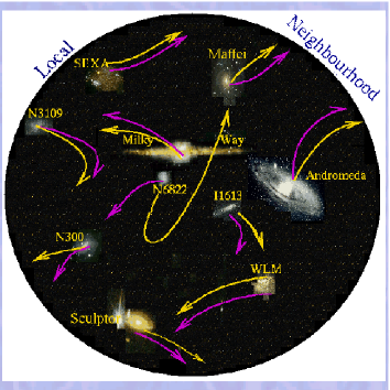
Figure 13: A schematic demonstration of Peebles’ reconstruction of the trajectories of the members of the local neighbourhood using a variational approach based on the minimization of Euler–Lagrange action. The arrows go back in time, starting from the present and pointing towards the initial positions of the sources. In most cases there is more than one allowed trajectory due to orbit crossing (closely related to the multi-streaming of the underlying dark matter fluid). The pink (darker) orbits correspond to taking the minimum of the action whereas the yellow (brighter) orbits were obtained by taking the saddle-point solution. Of particular interest is the orbit of N6822 which in the former solution is on its first approach towards us and in the second solution is in its passing orbit. A better agreement between the evaluated and observed velocities was shown to correspond to the saddle-point solution.

This led Peebles (1990) to partially relax the assumption of minimum action, allowing also for saddle points in the action. Somewhat better agreement with observations is then obtained, but at the expense of lack of uniqueness.

In the context of the present approach, various remarks can be made. The boundary condition (59) is trivially satisfied if the velocities $d{\mn@boldsymbol{x}}/d\tau$ remain bounded. Actually, we have seen in Section 2.1 that, as a consequence of slaving, the velocity has a regular expansion in powers of $\tau$, which implies its boundedness as $\tau\to 0$. The important point is that the function $f_{n}(\tau)$ appearing in (60) should be expandable in powers of $\tau$, as is the case with the ansatz (61).

In Section 6 we have established uniqueness of the reconstruction with a prescribed present density and under the assumption of absence of multi-streaming (but we allow for mass concentrations). This restriction is meaningful only in the continuous case: in the discrete case, unless the particles are rather closely packed, the concept of multi-streaming is not clear but there have been attempts to relate uniqueness to absence of ‘orbit crossing’ (see, e.g., Giavalisco et al., 1993; Whiting, 2000). Of course, at the level of the underlying dark matter, multi-streaming is certainly not ruled out at sufficiently small scales; at such scales unique reconstruction is not possible.

In the truly discrete case, e.g. when considering a dwarf galaxy, there is no reason to prefer the true minimum action solution over any other stationary action solution.

8 Conclusion

The main theoretical result of this paper is that reconstruction of the past dynamical history of the Universe, knowing only the present spatial distribution of mass, is a well-posed problem with a unique solution. More precisely, reconstruction is uniquely defined down to those scales, a few megaparsecs, where multi-streaming becomes important. The presence of concentrated mass in the form of clusters, filaments, etc is not an obstacle to a unique displacement reconstruction; the mass within each such structure originates from a collapsed region of known shape but with unknown initial density and velocity fluctuations inside. There are of course practical limitations to reconstruction stemming from the knowledge of the present mass distribution over only a limited patch of the Universe; these were discussed in Section 3.4.

In this paper we have also presented in detail and tested a reconstruction method called MAK which reduces reconstruction to an assignment problem with quadratic cost, for which effective algorithms are available. MAK, which is exact for dynamics governed by the adhesion model, works very well above $6\,h^{-1}$ Mpc and can in principle be adapted to full Euler–Poisson reconstruction.

We note that a very common method for testing ideas about the early Universe is to take some model of early density fluctuations and then run an $N$-body simulations with assumed cosmological parameters until the present epoch. Confrontation with the observed statistical properties of the present Universe helps then in selecting plausible models and in narrowing the choice of cosmological parameters. This forward method is conceptually very different from reconstruction; the latter not only works backward but, more importantly, it is a deterministic method which gives us a detailed map of the early Universe and how it relates to the present one. Reconstruction thus allows us to obtain the peculiar velocities of galaxies and is probably the only method which can hope to do this for a large number of galaxies. In those instances were we have partial information on peculiar velocities (from independent distance measurements), e.g. for the NearBy Galaxies (NBG) catalogue of Tully (1988), such information can be used to calibrate cosmological parameters or to provide additional constraints, which are in principle redundant but can improve the quality.

The detailed reconstruction of early density fluctuations, which will become possible using large 3D surveys such as 2dF and SDSS (see, e.g., Frieman & Szalay, 2000), will allow us to test such assumptions as the Gaussianity of density fluctuations at decoupling. Note however that such reconstruction gives us full access only to the complement of collapsed regions; any statistical information thus obtained will be biased, roughly by overemphasizing underdense regions.

Finally we have no reason to hide the pleasure we experience in seeing this heavenly problem bring together and indeed depend crucially on so many different areas of mathematics and physics, from fluid dynamics to Monge–Ampère equations, mass transportation, convex geometry and combinatorial optimization. Probably this is the first time that one tackles the three-dimensional Monge–Ampère equation numerically for practical purposes. As usual, we can expect that the techniques, here applied to cosmic reconstruction, will find many applications, for example to the optimal matching of two holographic or tomographic images or to the correction of images in multi-dimensional colour space.

Appendix A Equations of motion in an expanding universe

On distances covered by present and forthcoming redshift galaxy catalogues, the Newtonian description constitutes a realistic approximation to the dynamics of self-gravitating cold dark matter filling the Universe (Peebles, 1980; Coles & Lucchin, 2002). This description gives, in proper space coordinates denoted here by ${\mn@boldsymbol{r}}$ and cosmic time $t$, the familiar Euler–Poisson system for the density $\varrho({\mn@boldsymbol{r}},t)$, velocity ${\mn@boldsymbol{U}}({\mn@boldsymbol{r}},t)$ and the gravitational potential $\phi({\mn@boldsymbol{r}},t)$:

$$\partial_{t}{\mn@boldsymbol{U}}+({\mn@boldsymbol{U}}\cdot\nabla_{\mn@boldsymbol{r}}){\mn@boldsymbol{U}} = -\nabla_{r}\phi_{\mathrm{g}},$$ (A.1)

$$\partial_{t}\varrho+\nabla_{\mn@boldsymbol{r}}\cdot(\varrho{\mn@boldsymbol{U}}) = 0,$$ (A.2)

$$\nabla^{2}_{\mn@boldsymbol{r}}\phi_{\mathrm{g}} = 4\pi G\varrho,$$ (A.3)

where $G$ is the gravitation constant.

In a homogeneous isotropic universe, the density and velocity fields take the form

$$\varrho({\mn@boldsymbol{r}},t)=\bar{\varrho}(t),\quad{\mn@boldsymbol{U}}({\mn@boldsymbol{r}},t)=H(t){\mn@boldsymbol{r}}=\frac{{\dot{a}}(t)}{a(t)}{\mn@boldsymbol{r}}.$$ (A.4)

Here the coefficient $H(t)$ is the Hubble parameter, and $a(t)$ is the expansion scale factor defined so that integration of the velocity field $\dot{\mn@boldsymbol{r}}={\mn@boldsymbol{U}}({\mn@boldsymbol{r}},t)=H(t){\mn@boldsymbol{r}}$ yields ${\mn@boldsymbol{r}}=a(t){\mn@boldsymbol{x}}$, where ${\mn@boldsymbol{x}}$ is called the comoving coordinate.

The background density $\bar{\varrho}(t)$ gives rise to the background gravitational potential $\bar{\phi}_{\mathrm{g}}$, which by (A.1) and (A.4) satisfies

$$-\nabla_{\mn@boldsymbol{r}}\bar{\phi}_{\mathrm{g}}=\frac{\ddot{a}}{a}{\mn@boldsymbol{r}}.$$ (A.5)

For the background density, mass conservation (A.2) gives then

$$\bar{\varrho}a^{3}=\bar{\varrho}_{0},$$ (A.6)

where $\bar{\varrho}_{0}=\bar{\varrho}(t_{0})$ with $t_{0}$ the present epoch and $a(t_{0})$ is normalized to unity. Eqs. (A.5), (A.6), and (A.3) imply the Friedmann equation for $a(t)$:

$$\ddot{a}=-\frac{4}{3}\pi G\bar{\varrho}_{0}\frac{1}{a^{2}}$$ (A.7)

with conditions posed at $t=t_{0}$:

$$a(t_{0})=1,\quad\dot{a}(t_{0})=H_{0}>0,$$ (A.8)

where $H_{0}$ is the present value of the Hubble parameter, positive for an expanding universe.

For simplicity we restrict ourselves to the case of the critical density, corresponding to the flat, matter-dominated Einstein-de Sitter universe (without a cosmological constant):

$$\bar{\varrho}_{0}=\frac{3H_{0}^{2}}{8\pi G}$$ (A.9)

and adjust the origin of the time axis such that the solution takes the form of a power law

$$a(t)=\left(\frac{t}{t_{0}}\right)^{2/3}$$ (A.10)

with $H_{0}=2/(3t_{0})$ and $\bar{\varrho}_{0}=1/(6\pi Gt_{0}^{2})$.

The observed Hubble expansion of the Universe suggests that the density, velocity and gravitational fields may be decomposed into a sum of terms describing the uniform expansion and fluctuations against the background:

$$\varrho=\bar{\varrho}(t)\,\rho,\quad{\mn@boldsymbol{U}}=\frac{\dot{a}(t)}{a(t)}{\mn@boldsymbol{r}}+a(t){\mn@boldsymbol{u}},\quad\phi_{\mathrm{g}}=\bar{\phi}_{\mathrm{g}}+\widetilde{\varphi}_{\mathrm{g}}.$$ (A.11)

The term $a(t){\mn@boldsymbol{u}}$ is called the peculiar velocity. In cosmology, one also often employs the density contrast defined as $\delta=\rho-1$, which gives the fluctuation against the normalized background density. Taking $\rho$, ${\mn@boldsymbol{u}}$, and $\widetilde{\varphi}_{\mathrm{g}}$ as functions of the comoving coordinate ${\mn@boldsymbol{x}}={\mn@boldsymbol{r}}/a(t)$ and using (A.5), (A.6) and (A.7), we rewrite the Euler–Poisson system in the form

$$\partial_{t}{\mn@boldsymbol{u}}+({\mn@boldsymbol{u}}\cdot{\nabla_{{\mn@boldsymbol{x}}}}){\mn@boldsymbol{u}} = -2\frac{\dot{a}}{a}{\mn@boldsymbol{u}}-\frac{1}{a}{\nabla_{{\mn@boldsymbol{x}}}}\widetilde{\varphi}_{\mathrm{g}},$$ (A.12)

$$\partial_{t}\rho+{\nabla_{{\mn@boldsymbol{x}}}}\cdot(\rho{\mn@boldsymbol{u}}) = 0,$$ (A.13)

$${\nabla^{2}_{{\mn@boldsymbol{x}}}}\widetilde{\varphi}_{\mathrm{g}} = \frac{4\pi G\bar{\varrho}_{0}}{a}(\rho-1).$$ (A.14)

Note the Hubble drag term $-2(\dot{a}/a){\mn@boldsymbol{u}}$ in the right-hand side of (A.12) representing the relative slowdown of peculiar velocities due to the uniform expansion.

Formally linearizing (A.12)–(A.14) around the trivial zero solution, one obtains the following ODE for the linear growth factor $\tau(t)$ of density fluctuations:

$$\frac{d}{dt}(a^{2}\dot{\tau})=4\pi G\bar{\varrho}_{0}\frac{\tau}{a}.$$ (A.15)

The only solution of this equation that stays bounded (indeed, vanishes) at small times is usually referred to as the growing mode. As we shall shortly see, it is convenient to choose the amplitude factor $\tau$ of the growing mode to be a new ‘time variable,’ which in an Einstein–de Sitter universe is proportional to $t^{2/3}$. It is normalized such that $\tau_{0}=\tau(t_{0})=1$. Rescaling the peculiar velocity and the gravitational potential according to

$${\mn@boldsymbol{u}}=\dot{\tau}{\mn@boldsymbol{v}},\quad\widetilde{\varphi}_{\mathrm{g}}=\frac{4\pi G\bar{\varrho}_{0}\tau}{a}\varphi_{\mathrm{g}}$$ (A.16)

and using the fact that in an Einstein–de Sitter universe $d\ln(a^{2}\dot{\tau})/d\tau=3/(2\tau)$, we arrive at the following form of the Euler–Poisson system, which we use throughout this paper:

$${\partial_{\tau}}{\mn@boldsymbol{v}}+({\mn@boldsymbol{v}}\cdot{\nabla_{{\mn@boldsymbol{x}}}}){\mn@boldsymbol{v}} = -\frac{3}{2\tau}({\mn@boldsymbol{v}}+{\nabla_{{\mn@boldsymbol{x}}}}\varphi_{\mathrm{g}}),$$ (A.17)

$${\partial_{\tau}}\rho+{\nabla_{{\mn@boldsymbol{x}}}}\cdot(\rho{\mn@boldsymbol{v}}) = 0,$$ (A.18)

$${\nabla^{2}_{{\mn@boldsymbol{x}}}}\varphi_{\mathrm{g}} = \frac{\rho-1}{\tau}.$$ (A.19)

Suppose initially, i.e. at $\tau=0$, a mass element is located at a point with the comoving coordinate ${\mn@boldsymbol{q}}$. Transported by the peculiar velocity field in the comoving coordinates, this element describes a trajectory ${\mn@boldsymbol{x}}({\mn@boldsymbol{q}},\tau)$. Using the Lagrangian coordinate ${\mn@boldsymbol{q}}$ to parametrize the whole continuum of mass elements, we recast (A.17) and (A.19) in the form

$${D^{2}_{\tau}}{\mn@boldsymbol{x}} = -\frac{3}{2\tau}\left({D_{\tau}}{\mn@boldsymbol{x}}+{\nabla_{{\mn@boldsymbol{x}}}}\varphi_{\mathrm{g}}\right),$$ (A.20)

$${\nabla^{2}_{{\mn@boldsymbol{x}}}}\varphi_{\mathrm{g}} = \frac{1}{\tau}\left[\left(\det{\nabla_{{\mn@boldsymbol{q}}}}{\mn@boldsymbol{x}}\right)^{-1}-1\right].$$ (A.21)

The density and peculiar velocity in Lagrangian variables are given by

$$\begin{array}[]{r@{{}={}}l}\rho({\mn@boldsymbol{x}}({\mn@boldsymbol{q}},\tau),\tau)&\left(\det{\nabla_{{\mn@boldsymbol{q}}}}{\mn@boldsymbol{x}}\right)^{-1},\\[4.30554pt] {\mn@boldsymbol{v}}({\mn@boldsymbol{x}}({\mn@boldsymbol{q}},\tau),\tau)&{D_{\tau}}{\mn@boldsymbol{x}}({\mn@boldsymbol{q}},\tau),\end{array}$$ (A.22)

which automatically satisfy the mass conservation law (A.18). Here ${D_{\tau}}$ is the operator of Lagrangian time derivative, which in Lagrangian variables is the usual partial time derivative at constant ${\mn@boldsymbol{q}}$ and in Eulerian variables coincides with the material derivative ${\partial_{\tau}}+{\mn@boldsymbol{v}}\cdot{\nabla_{{\mn@boldsymbol{x}}}}$. The notation ${\nabla_{{\mn@boldsymbol{x}}}}$ in Lagrangian variables stands for the ${\mn@boldsymbol{x}}({\mn@boldsymbol{q}},\tau)$-dependent differential operator with components $\nabla_{x_{i}}\equiv(\partial{q_{j}}/\partial{x_{i}})\nabla_{q_{j}}$, which expresses the Eulerian gradient rewritten in Lagrangian coordinates, using the inverse Jacobian matrix. Note that ${\nabla_{{\mn@boldsymbol{x}}}}$ and ${D_{\tau}}$ do not commute and that terms with ${\nabla_{{\mn@boldsymbol{x}}}}$ in the Lagrangian equations are implicitly non-linear.

In one dimension, (A.21) has an interesting consequence:

$$\nabla_{x}\varphi_{\mathrm{g}}=-\frac{x-q}{\tau}.$$ (A.23)

Indeed, in one dimension (A.21) takes the form

$$\nabla^{2}_{x}\varphi_{\mathrm{g}}=\frac{1}{\tau}\left[\left(\nabla_{q}x\right)^{-1}-1\right].$$ (A.24)

Multiplying this equation by $\nabla_{q}x$ and expressing the first of the two $x$-derivatives acting on $\varphi_{\mathrm{g}}$ as a $q$-derivative, we obtain

$$\nabla_{q}\left(\nabla_{x}\varphi_{\mathrm{g}}\right)=\nabla_{q}\frac{q-x}{\tau}.$$ (A.25)

Eq. (A.23) is obtained from (A.25) by integrating in $q$. The absence of an arbitrary $\tau$-dependent constant is established either by assuming vanishing at large distances of both $\varphi_{\mathrm{g}}$ and of the displacement $x-q$ or, in the space-periodic case, by assuming the vanishing of period averages.

Using (A.23) to eliminate the $\varphi_{\mathrm{g}}$ term in (A.20) and introducing the notation $\xi$ for the displacement $x-q$, we obtain

$${D^{2}_{\tau}}\xi=-\frac{3}{2\tau}\left({D_{\tau}}\xi-\frac{\xi}{\tau}\right).$$ (A.26)

The only solution to this equation that remains well-behaved for $\tau\to 0$ is the linear one $\xi\propto\tau$. This solution has the two terms on the right-hand side of the one-dimensional version of (A.20) cancelling each other and hence gives a vanishing ‘acceleration’ ${D^{2}_{\tau}}x$.

An approximate vanishing of acceleration takes place in higher dimensions as well. For early times, the Lagrangian map ${\mn@boldsymbol{x}}({\mn@boldsymbol{q}},\tau)$ stays close to the identity, with displacements ${\mn@boldsymbol{\xi}}({\mn@boldsymbol{q}},\tau)={\mn@boldsymbol{x}}({\mn@boldsymbol{q}},\tau)-{\mn@boldsymbol{q}}$ small. Linearizing (A.20) and (A.21) around zero displacement, we get the system

$${D^{2}_{\tau}}{\mn@boldsymbol{\xi}} = -\frac{3}{2\tau}({D_{\tau}}{\mn@boldsymbol{\xi}}+{\nabla_{{\mn@boldsymbol{q}}}}\varphi_{\mathrm{g}}),$$ (A.27)

$${\nabla^{2}_{{\mn@boldsymbol{q}}}}\varphi_{\mathrm{g}} = -\frac{1}{\tau}{\nabla_{{\mn@boldsymbol{q}}}}\cdot{\mn@boldsymbol{\xi}}.$$ (A.28)

Here we use the fact that ${\nabla_{{\mn@boldsymbol{x}}}}\simeq{\nabla_{{\mn@boldsymbol{q}}}}$ and $\det{\nabla_{{\mn@boldsymbol{q}}}}{\mn@boldsymbol{x}}\simeq\hbox{$1+{\nabla_{{\mn@boldsymbol{q}}}}\cdot{\mn@boldsymbol{\xi}}$}$. Using (A.28) to eliminate $\varphi_{\mathrm{g}}$ in (A.27), we get for $\theta\equiv{\nabla_{{\mn@boldsymbol{q}}}}\cdot{\mn@boldsymbol{\xi}}$ an equation that coincides with (A.26) up to the change of variable $\xi\mapsto\theta$. Choosing the well-behaved linear solution for $\theta$, solving for ${\mn@boldsymbol{\xi}}$ and using the above argument to eliminate a $\tau$-dependent constant, we see that, in the linearized equations, terms in the right-hand side of (A.27) cancel each other and the acceleration vanishes. This simplification justifies using the linear growth factor $\tau$ as a time variable.

Appendix B History of mass transportation

The subject of mass transportation was started by Gaspard Monge (1781) in a paper entitled Théorie des déblais et des remblais (Theory of cuts and fills) whose preamble is worth quoting entirely (our translation):

   When earth is to be moved from one place to another, the usage is to call cuts the volumes of earth to be transported and fills the space to be occupied after transportation.

    The cost of transporting one molecule being, all things otherwise equal, proportional to its weight and to the distance [espace] travelled and consequently the total cost being proportional to the sum of products of molecules each multiplied by the distance travelled, it follows that for given shapes and positions of the cuts and fills, it is not indifferent that any given molecule of the cuts be transported to this or that place in the fills, but there ought to be a certain distribution of molecules of the former into the latter, according to which the sum of these products will be the least possible, and the cost of transportation will be a minimum.

Although clearly posed, the ‘mass transportation problem’ was not solved, in more than one dimension, until Leonid Kantorovich (1942) formulated a ‘relaxed’ version, now called the Monge–Kantorovich problem: instead of a ‘distribution of molecules of the former into the latter,’ he allowed a distribution in the product space where more than one position in the fills could be associated with a position in the cuts and where the initial and final distributions are prescribed marginals (see Section 3.3). In cosmospeak, he allowed multi-streaming with given initial and final mass distributions. Using the techniques of duality and of linear programming that he had invented (see Appendix C.2), Kantorovich was then able to solve the mass transportation problem in this relaxed formulation. The techniques developed by Kantorovich found many applications, notably in economics, which in fact was his original motivation (he was awarded, together with T.C. Koopmans, the 1975 Nobel prize in this field).

Before turning to more recent developments we must say a few words about the history of the Monge–Ampère equation. It was considered for the first time by Ampère (1820) for an unknown function $z(x,y)$ of two scalar variables. The equation is to be found on p. 65 of Ampère’s huge (188 pages) mathematical memoir in the form

$$Hr+2Ks+Lt+M+N(rt-s^{2})=0,$$ (B.1)

where in modern notation $r=\partial^{2}z/\partial x^{2}$, $s=\partial^{2}z/(\partial x\partial y)$, $t=\partial^{2}z/\partial y^{2}$, and $H,K,L,M,N$ are functions of $x,y,z$ and the two first-order derivatives $p=\partial z/\partial x$ and $q=\partial z/\partial y$. This extends the earlier work by Monge (1784, see p. 126) concerning the equation without the Hessian term ($N=0$). Both Ampère and Monge were interested in methods of explicit integration of these equations. Ampère also pointed out the way the equation changes under Legendre transformations but there is no physical interpretation in terms of Lagrangian coordinates. There is evidence that until the beginning of the 20th century the scientific community attributed the equation with the Hessian solely to Ampère Bour (1862, p. 186) and Weber (1900, p. 367). But the joint attribution of (B.1) to ‘Monge and Ampère’ is already found in (Goursat, 1896).

The subjects of mass transportation and of the Monge–Ampère equation came together when one of us (YB) showed the equivalence of the elliptic Monge–Ampère equation and of the mass transportation problem with quadratic cost: when initial and final distributions are non-singular, the optimal solution is actually one-to-one, so that nothing is lost by the Kantorovich relaxation trick (Brenier, 1987, 1991). For an extension of this result to general costs see Gangbo & McCann (1996); a review of the many recent papers on the subject is given by Ambrosio (2003).

Appendix C Basics of convexity and duality

C.1 Convexity and the Legendre transformation

A convex body may be defined by the condition that it coincides with the intersection of all half-spaces containing it. Obviously, it is sufficient to take only those half-spaces limited by planes that touch the body; such planes are called supporting.

Take now a convex function $f({\mn@boldsymbol{q}})$, so that the set of points in the $(3+1)$-dimensional $({\mn@boldsymbol{q}},f)$ space lying above its graph is convex. It follows that we can write

$$f({\mn@boldsymbol{q}})=\max_{\mn@boldsymbol{x}}\,{\mn@boldsymbol{x}}\cdot{\mn@boldsymbol{q}}-f^{*}({\mn@boldsymbol{x}}),$$ (C.2)

where the expression ${\mn@boldsymbol{x}}\cdot{\mn@boldsymbol{q}}-f^{*}({\mn@boldsymbol{x}})$ specifies a supporting plane with the slope ${\mn@boldsymbol{x}}$ for the set of points lying above the graph of $f$ (see Fig. 14 for the one-dimensional case).

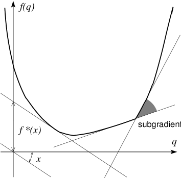
Figure 14: A convex function $f(q)$ and the geometrical construction of its Legendre transform $f^{*}(x)$. Also illustrated is the subgradient of $f(q)$ at a non-smooth point.

The function $f^{*}({\mn@boldsymbol{x}})$, which specifies how high one should place a supporting plane to touch the graph, is called the Legendre transform of $f({\mn@boldsymbol{q}})$.

From Eq. (C.2) follows the inequality (known as the Young inequality)

$$f({\mn@boldsymbol{q}})+f^{*}({\mn@boldsymbol{x}})\geq{\mn@boldsymbol{x}}\cdot{\mn@boldsymbol{q}}\mbox{ for all ${\mn@boldsymbol{x}}$, ${\mn@boldsymbol{q}}$,}$$ (C.3)

where both sides coincide if and only if the supporting plane with the slope ${\mn@boldsymbol{x}}$ touches the graph of $f$ at ${\mn@boldsymbol{q}}$. This fact, together with the obvious symmetry of this inequality, implies that

$$f^{*}({\mn@boldsymbol{x}})=\max_{\mn@boldsymbol{q}}\,{\mn@boldsymbol{x}}\cdot{\mn@boldsymbol{q}}-f({\mn@boldsymbol{q}}).$$ (C.4)

Thus, the Legendre transform of a convex function is itself convex and the Legendre transform of the Legendre transform recovers the initial convex function.

If however we apply (C.2) to a nonconvex function $f$, we obtain a convex function $f^{*}$, whose own Legendre transform will give the convex hull of $f$, the largest convex function whose graph lies below that of $f$.

When $f$ is both convex and differentiable, (C.3) becomes an equality for ${\mn@boldsymbol{x}}={\nabla_{{\mn@boldsymbol{q}}}}f({\mn@boldsymbol{q}})$. If $f^{*}$ is also differentiable, then one also has ${\mn@boldsymbol{q}}={\nabla_{{\mn@boldsymbol{x}}}}f^{*}({\mn@boldsymbol{x}})$. This is actually Legendre’s original definition of the transformation, which is thus limited to smooth functions. Furthermore, if the original function is not convex and thus has the same gradient at separated locations, Legendre’s purely local definition will give a multivalued Legendre transform. (In the context of the present paper this corresponds to multi-streaming.)

Not all convex functions are differentiable (e.g. $f({\mn@boldsymbol{q}})=|{\mn@boldsymbol{q}}|$). But the Young inequality can be employed to define a useful generalization of the gradient: the subgradient of $f$ at ${\mn@boldsymbol{q}}$ is the set of all ${\mn@boldsymbol{x}}$ for which the equality in (C.3) holds (see Fig. 14). If $f$ is smooth at ${\mn@boldsymbol{q}}$, then ${\nabla_{{\mn@boldsymbol{q}}}}f({\mn@boldsymbol{q}})$ will be the only such point; otherwise, there will be a (convex) set of them.

If a convex function has the same subgradient at more than one point, the function is said to lack strict convexity. In fact, strict convexity and smoothness are complementary: lack of one in a convex function implies lack of the other in the Legendre transform.

For further background on convex analysis and geometry, see Rockafellar (1970).

C.2 Duality in optimization

Suppose we want to minimize a convex function $\Phi({\mn@boldsymbol{q}})$ subject to a set of linear constraints that may be written in matrix notation as $A{\mn@boldsymbol{q}}={\mn@boldsymbol{b}}$ (vectors ${\mn@boldsymbol{q}}$ satisfying this constraint are called admissible in optimization parlance). We now observe that

$$\inf_{A{\mn@boldsymbol{q}}={\mn@boldsymbol{b}}}\Phi({\mn@boldsymbol{q}})=\mathop{\mathrm{inf\vphantom{p}}}_{{\mn@boldsymbol{q}}}\sup_{{\mn@boldsymbol{x}}}\,\Phi({\mn@boldsymbol{q}})-{\mn@boldsymbol{x}}\cdot(A{\mn@boldsymbol{q}}-{\mn@boldsymbol{b}}).$$ (C.5)

Indeed, should $A{\mn@boldsymbol{q}}$ not equal ${\mn@boldsymbol{b}}$, the $\sup$ operation in ${\mn@boldsymbol{x}}$ will give infinity, so such ${\mn@boldsymbol{q}}$ will not contribute to minimization. Here we use the $\inf$/$\sup$ notation instead of $\min$/$\max$ because the extremal values may not be reached, e.g., when they are infinite.

Using (C.2), we rewrite this in the form

$$\begin{array}[]{@{}l@{}}\displaystyle\mathop{\mathrm{inf\vphantom{p}}}_{{\mn@boldsymbol{q}}}\sup_{{\mn@boldsymbol{x}},{\mn@boldsymbol{y}}}\,{\mn@boldsymbol{y}}\cdot{\mn@boldsymbol{q}}-\Phi^{*}({\mn@boldsymbol{y}})-{\mn@boldsymbol{x}}\cdot(A{\mn@boldsymbol{q}}-{\mn@boldsymbol{b}})\\ \displaystyle=\mathop{\mathrm{inf\vphantom{p}}}_{{\mn@boldsymbol{q}}}\sup_{{\mn@boldsymbol{x}},{\mn@boldsymbol{y}}}\,({\mn@boldsymbol{y}}-A^{T}{\mn@boldsymbol{x}})\cdot{\mn@boldsymbol{q}}-\Phi^{*}({\mn@boldsymbol{y}})+{\mn@boldsymbol{x}}\cdot{\mn@boldsymbol{b}},\end{array}$$ (C.6)

where $\Phi^{*}({\mn@boldsymbol{y}})$ is the Legendre transform of $\Phi({\mn@boldsymbol{q}})$ and $A^{T}$ is the transpose of $A$. Taking $\inf$ in ${\mn@boldsymbol{q}}$ first, we see that the expression in the right-hand side will be infinite unless ${\mn@boldsymbol{y}}=A^{T}{\mn@boldsymbol{x}}$. We then obtain the optimization problem of finding

$$\sup_{{\mn@boldsymbol{x}}}\,{\mn@boldsymbol{x}}\cdot{\mn@boldsymbol{b}}-\Phi^{*}(A^{T}{\mn@boldsymbol{x}}),$$ (C.7)

which is called dual to the original one. Note that there are no constraints on the dual variable ${\mn@boldsymbol{x}}$: any value is admissible.

Denoting solutions of problems (C.5) and (C.7) by ${\mn@boldsymbol{q}}^{*}$ and ${\mn@boldsymbol{x}}^{*}$, we see that

$$\Phi({\mn@boldsymbol{q}}^{*})+\Phi^{*}(A^{T}{\mn@boldsymbol{x}}^{*})-{\mn@boldsymbol{x}}^{*}\cdot{\mn@boldsymbol{b}}=0,$$ (C.8)

because the optimal values of both problems are given by (C.6) and thus coincide. Furthermore, for any admissible ${\mn@boldsymbol{q}}$ and ${\mn@boldsymbol{x}}$

$$\Phi({\mn@boldsymbol{q}})+\Phi^{*}(A^{T}{\mn@boldsymbol{x}})-{\mn@boldsymbol{x}}\cdot{\mn@boldsymbol{b}}\geq 0,$$ (C.9)

because the right-hand sides of (C.5) and (C.7) cannot pass beyond their optimal values.

Moreover, let equality (C.8) be satisfied for some admissible ${\mn@boldsymbol{q}}^{*}$ and ${\mn@boldsymbol{x}}^{*}$; then such ${\mn@boldsymbol{q}}^{*}$ and ${\mn@boldsymbol{x}}^{*}$ must solve the problems (C.5) and (C.7). Indeed, taking e.g. ${\mn@boldsymbol{x}}^{*}$ for ${\mn@boldsymbol{x}}$ in (C.9) and using (C.8), we see that for any other admissible ${\mn@boldsymbol{q}}$

$$\Phi({\mn@boldsymbol{q}}^{*})\leq\Phi({\mn@boldsymbol{q}}),$$ (C.10)

i.e., that ${\mn@boldsymbol{q}}^{*}$ solves the original optimization problem (C.5).

Convex optimization problems with linear constraints considered in this section are called convex programs. Their close relatives are linear programs, namely optimization problems of the form

$$\inf_{A{\mn@boldsymbol{q}}={\mn@boldsymbol{b}},\,{\mn@boldsymbol{q}}\geq 0}{\mn@boldsymbol{c}}\cdot{\mn@boldsymbol{q}}=\mathop{\mathrm{inf\vphantom{p}}}_{{\mn@boldsymbol{q}}\geq 0}\sup_{{\mn@boldsymbol{x}}}\,{\mn@boldsymbol{c}}\cdot{\mn@boldsymbol{q}}-{\mn@boldsymbol{x}}\cdot(A{\mn@boldsymbol{q}}-{\mn@boldsymbol{b}}),$$ (C.11)

where notation ${\mn@boldsymbol{q}}\geq 0$ means that all components of the vector ${\mn@boldsymbol{q}}$ are nonnegative. Proceeding essentially as above with ${\mn@boldsymbol{c}}\cdot{\mn@boldsymbol{q}}$ instead of $\Phi({\mn@boldsymbol{q}})$, we observe that in order not to obtain infinity when minimizing in ${\mn@boldsymbol{q}}$ in (C.6), we have now to require that $A^{T}{\mn@boldsymbol{x}}\leq{\mn@boldsymbol{c}}$ (i.e. ${\mn@boldsymbol{c}}-A^{T}{\mn@boldsymbol{x}}\geq 0$). The dual problem thus takes the form

$$\sup_{A^{T}{\mn@boldsymbol{x}}\leq{\mn@boldsymbol{c}}}\,{\mn@boldsymbol{x}}\cdot{\mn@boldsymbol{b}}$$ (C.12)

with an admissibility constraint on ${\mn@boldsymbol{x}}$. Instead of (C.8) and (C.9) we obtain

$${\mn@boldsymbol{x}}^{*}\cdot{\mn@boldsymbol{b}}={\mn@boldsymbol{c}}\cdot{\mn@boldsymbol{q}}^{*}\quad\mbox{or}\quad(A^{T}{\mn@boldsymbol{x}}^{*}-{\mn@boldsymbol{c}})\cdot{\mn@boldsymbol{q}}^{*}=0$$ (C.13)

and

$${\mn@boldsymbol{x}}\cdot{\mn@boldsymbol{b}}\leq{\mn@boldsymbol{c}}\cdot{\mn@boldsymbol{q}}\quad\mbox{or}\quad(A^{T}{\mn@boldsymbol{x}}-{\mn@boldsymbol{c}})\cdot{\mn@boldsymbol{q}}\leq 0,$$ (C.14)

the latter inequality being automatically satisfied for any admissible ${\mn@boldsymbol{x}},{\mn@boldsymbol{q}}$. Note that for linear programs, the fact that (C.13) holds for some admissible ${\mn@boldsymbol{q}}^{*},{\mn@boldsymbol{x}}^{*}$ also implies that ${\mn@boldsymbol{q}}^{*}$ and ${\mn@boldsymbol{x}}^{*}$ solve their respective optimization problems.

For further background on optimization and duality, see, e.g., Papadimitriou & Steiglitz (1982).

C.3 Why the analogue computer of Section 4.2 solves the assignment problem

We suppose that the analogue computer described in Section 4.2 has settled into equilibrium, which minimizes its potential energy

$$U=\sum_{i=1}^{N}\alpha_{i}-\sum_{j=1}^{N}\beta_{j},$$ (C.15)

under the set of constraints

$$\alpha_{i}-\beta_{j}\geq C-c_{ij},$$ (C.16)

for all $i,j$. Our goal is here is to show that the set of equilibrium forces $f_{ij}$, acting on studs between row and column rods, solves the original linear programming problem of minimizing

$$\tilde{I}=\sum_{i,j=1}^{N}c_{ij}f_{ij}$$ (C.17)

under constraints

$$f_{ij}\geq 0,\qquad\sum_{k=1}^{N}f_{kj}=\sum_{k=1}^{N}f_{ik}=1,$$ (C.18)

for all $i,j$ and that in fact forces $f_{ij}$ take only zero and unit values, thus providing the solution to the assignment problem.

Note first that if a row rod $A_{i}$ and a column rod $B_{j}$ are not in contact at equilibrium, then the corresponding force vanishes ($f_{ij}=0$); if they are, then $f_{ij}\geq 0$. Take now a particular pair of rods $A_{i}$ and $B_{j}$ that are in contact. At equilibrium, the force $f_{ij}$ must equal forces exerted on the corresponding stud by $A_{i}$ and $B_{j}$. We claim that both these forces must be integer. To see this, let us compute the force exerted by $A_{i}$. This rod contributes its weight, $+1$, possibly decreased by the force that it feels from other column rods that are in contact with $A_{i}$. Each of these takes $-1$ (its ‘buoyancy’) out of the total force, but we may have to add the force it feels in turn from other row rods with which it might be in contact. Proceeding this way from one rod to another, we see that all contributions, positive or negative, are unity, so their sum $f_{ij}$ must be integer. The same argument applies to rod $B_{j}$.

Does this process indeed finish or, at some stage, do we come back at an already visited stud and thus end up in an infinite cycle? In fact, for general set of stud lengths $C-c_{ij}$, the latter cannot happen, because otherwise an alternating sum of some subset of stud lengths would give exactly zero – a zero probability event for a set of arbitrary real numbers.

Consider now a row rod $A_{i}$. It is in contact with one or more column rods, whose combined upward push must equilibrate the unit weight of $A_{i}$. Since any of the latter rods exerts a nonnegative integer force, it follows that exactly one of these forces is unity, and all the other ones are zero. A similar argument holds for any column rod $B_{j}$.

We have thus shown that all $f_{ij}$ in the equilibrium equal 1 or 0. One can of course ignore the vanishing forces. Then each row rod $A_{i}$ is supported by exactly one column rod $B_{j}$, and each $B_{j}$ supports exactly one $A_{i}$. This defines a one-to-one pairing, and we are only left with a check that this pairing minimizes (C.17).

Observe that pushing a column rod down by some distance $\Delta$ and simultaneously increasing by $\Delta$ the length of all studs attached to this rod will have no effect on positions and constraints of all other rods, hence on the equilibrium network of contacts. Moreover, due to constraints (C.18), the corresponding change in coefficients $c_{ij}$ will not change the cost function (C.17) in any essential way, except of just subtracting $\Delta$.

We can use this observation to put all column rods at the same level, say at $z=0$, adjusting $c_{ij}$ to some new values $c^{\prime}_{ij}$. Thus, for every $i$, the row rod $A_{i}$ rests on the stud with the largest height $C-c^{\prime}_{ij}$, so the equilibrium pairing maximizes the sum

$$\sum_{i,j=1}^{N}(C-c^{\prime}_{ij})f_{ij}$$ (C.19)

and thus minimizes (C.17).

Appendix D Details of the variational technique for the Euler–Poisson system

In this appendix, we explain details of the variational procedure outlined in Section 6, which proves that prescription of the density fields at terminal epochs $\tau=0$ and $\tau=\tau_{0}$ uniquely determines a regular and thus curl-free solution to the Euler–Poisson system (A.17)–(A.19).

The variational problem is posed for the functional

$$I=\frac{1}{2}\int_{0}^{\tau_{0}}\mathrm{d}\tau\int\mathrm{d}^{3}{\mn@boldsymbol{x}}\,\tau^{3/2}\left(\rho|{\mn@boldsymbol{v}}|^{2}+\frac{3}{2}|{\nabla_{{\mn@boldsymbol{x}}}}\varphi_{\mathrm{g}}|^{2}\right)$$ (D.1)

with four constraints: the Poisson equation (A.19), which we repeat here for convenience,

$${\nabla^{2}_{{\mn@boldsymbol{x}}}}\varphi_{\mathrm{g}}=\frac{\rho-1}{\tau},$$ (D.2)

the mass conservation (A.18), also repeated here,

$${\partial_{\tau}}\rho+{\nabla_{{\mn@boldsymbol{x}}}}\cdot(\rho{\mn@boldsymbol{v}})=0,$$ (D.3)

and the two boundary conditions

$$\rho({\mn@boldsymbol{x}},0)=1\quad{\rm and}\quad\rho({\mn@boldsymbol{x}},\tau_{0})=\rho_{0}({\mn@boldsymbol{x}}).$$ (D.4)

In the sequel, we shall always denote by $\int\!\!\int$ the double integration over $0\leq\tau\leq\tau_{0}$ and over the whole space domain in ${\mn@boldsymbol{x}}$ provided that the integrand vanishes at infinity sufficiently fast, or over the periodicity box in the case of periodic boundary conditions. A single integral sign $\int$ will always denote the integration over the relevant space domain in ${\mn@boldsymbol{x}}$.

First, we make this problem convex by rewriting the functional and constraints in a new set of variables with the mass flux ${\mn@boldsymbol{J}}({\mn@boldsymbol{x}},t)=\rho({\mn@boldsymbol{x}},t)\,{\mn@boldsymbol{v}}({\mn@boldsymbol{x}},t)$ instead of the velocity ${\mn@boldsymbol{v}}$. The mass conservation constraint, which was the only non-linear one in the old variables, becomes now linear:

$${\partial_{\tau}}\rho+{\nabla_{{\mn@boldsymbol{x}}}}\cdot{\mn@boldsymbol{J}}=0,$$ (D.5)

and one can check that the density of kinetic energy takes the form

$$\frac{1}{2}\rho|{\mn@boldsymbol{v}}|^{2}=\frac{1}{2\rho}|{\mn@boldsymbol{J}}|^{2}=\max_{c,\,{\mn@boldsymbol{m}}\colon\,\,c+|{\mn@boldsymbol{m}}|^{2}/2\leq 0}\,(\rho c+{\mn@boldsymbol{J}}\cdot{\mn@boldsymbol{m}})$$

or

$$\frac{|{\mn@boldsymbol{J}}|^{2}}{2\rho}=\max_{c,\,{\mn@boldsymbol{m}}}\,(\rho c+{\mn@boldsymbol{J}}\cdot{\mn@boldsymbol{m}}-F(c,{\mn@boldsymbol{m}})),$$ (D.6)

where

$$F(c,{\mn@boldsymbol{m}})=\cases{0&if $c+|{\mn@boldsymbol{m}}|^{2}/2\leq 0$\cr+\infty&otherwise.\cr}$$ (D.7)

Note that in (D.6) the variables $c,{\mn@boldsymbol{m}}$, as well as $\rho,{\mn@boldsymbol{J}}$, are functions of $({\mn@boldsymbol{x}},\tau)$. The action functional may now be written as

$$I=\frac{1}{2}\int\!\!\int\left(\frac{1}{\rho}|{\mn@boldsymbol{J}}|^{2}+\frac{3}{2}|{\nabla_{{\mn@boldsymbol{x}}}}\phi|^{2}\right)\tau^{3/2}\,\mathrm{d}^{3}{\mn@boldsymbol{x}}\,\mathrm{d}\tau,$$ (D.8)

and turns out to be convex.

To see this, first note that the operation of integration is linear and thus preserves convexity of the integrand. The integrand is a positive quadratic function of ${\nabla_{{\mn@boldsymbol{x}}}}\phi$ and therefore is convex in $\phi$; furthermore, (D.6) implies that it is also convex in $(\rho,{\mn@boldsymbol{J}})$, since the kinetic energy density $|{\mn@boldsymbol{J}}|^{2}/2\rho$ is the Legendre transform of the function $F(c,{\mn@boldsymbol{m}})$, which itself is convex.

Note also that by representing the kinetic energy density in the form (D.6), we may safely allow $\rho$ to take negative values: the right-hand side being in that case $+\infty$, it will not contribute to minimizing (D.1).

We now derive the dual optimization problem. We introduce the scalar Lagrange multipliers $\psi({\mn@boldsymbol{x}},t)$, $\vartheta_{\mathrm{in}}({\mn@boldsymbol{x}})$, $\vartheta_{0}({\mn@boldsymbol{x}})$ and $\theta({\mn@boldsymbol{x}},t)$ for the Poisson equation (D.2), the boundary conditions (D.4), and the constraints of mass conservation (D.5), respectively, and observe that the variational problem may now be written in the form

$$\begin{array}[]{@{}l@{}}\displaystyle\inf_{\begin{array}[]{@{}c@{}}\rule{0.0pt}{10.5pt}\scriptstyle\rho,{\mn@boldsymbol{J}},\phi\\ \end{array}}\;\sup_{\begin{array}[]{@{}c@{}}\scriptstyle c,{\mn@boldsymbol{m}},\theta,\psi,\vartheta_{0},\vartheta_{T}\colon\\ \scriptstyle c+|{\mn@boldsymbol{m}}|^{2}/2\leq 0\end{array}}\int\!\!\int\mathrm{d}^{3}{\mn@boldsymbol{x}}\,\mathrm{d}\tau\left[\frac{3}{2}\psi\left({\nabla^{2}_{{\mn@boldsymbol{x}}}}\phi-\frac{\rho-1}{\tau}\right)\right.\\ \displaystyle\quad\left.+\theta({\partial_{\tau}}\rho+{\nabla_{{\mn@boldsymbol{x}}}}\cdot{\mn@boldsymbol{J}})+\tau^{3/2}\left(\rho c+{\mn@boldsymbol{J}}\cdot{\mn@boldsymbol{m}}+\frac{3}{4}|{\nabla_{{\mn@boldsymbol{x}}}}\phi|^{2}\right)\right]\\ \displaystyle\quad+\int\vartheta_{\mathrm{in}}({\mn@boldsymbol{x}})(\rho({\mn@boldsymbol{x}},0)-1)\,\mathrm{d}^{3}{\mn@boldsymbol{x}}\\ \displaystyle\quad-\int\vartheta_{0}({\mn@boldsymbol{x}})(\rho({\mn@boldsymbol{x}},\tau_{0})-\rho_{0}({\mn@boldsymbol{x}}))\,\mathrm{d}^{3}{\mn@boldsymbol{x}}.\end{array}$$ (D.9)

To see that (D.9) is indeed equivalent to minimizing (D.1) under the constraints (D.3) or (D.5), (D.2), and (D.4), observe that for those $\rho,{\mn@boldsymbol{J}},\phi$ that do not satisfy the constraints, the $\sup$ operation over $\theta,\psi,\vartheta_{\mathrm{in}},\vartheta_{0}$ will give positive infinity; the $\sup$ will be finite (and thus contribute to the subsequent minimization) only if all constraints are satisfied. (This argument is the functional version of what is explained in Appendix C.2 for the finite-dimensional case.)

Performing an integration by parts in the $\tau$ variable in (D.9) and using the boundary conditions on the mass density (D.4), we find that $\vartheta_{\mathrm{in}}({\mn@boldsymbol{x}})=\theta({\mn@boldsymbol{x}},0)$ and $\vartheta_{0}({\mn@boldsymbol{x}})=\theta({\mn@boldsymbol{x}},\tau_{0})$. Integrating further by parts in the ${\mn@boldsymbol{x}}$ variable, assuming that boundary terms at infinity vanish (or that we have periodic boundary conditions in space) and rearranging terms, we get

$$\begin{array}[]{@{}l@{}}\displaystyle\inf_{\begin{array}[]{@{}c@{}}\rule{0.0pt}{10.5pt}\scriptstyle\rho,{\mn@boldsymbol{J}},\phi\\ \end{array}}\!\sup_{\begin{array}[]{@{}c@{}}\scriptstyle c,{\mn@boldsymbol{m}},\theta,\psi\colon\\[-1.50694pt] \scriptstyle c+|{\mn@boldsymbol{m}}|^{2}/2\leq 0\end{array}}\int\!\!\int\mathrm{d}^{3}{\mn@boldsymbol{x}}\,\mathrm{d}\tau\left(\rho\,(c\tau^{3/2}-{\partial_{\tau}}\theta-\frac{3}{2\tau}\psi)\right.\\ \displaystyle\qquad+{\mn@boldsymbol{J}}\cdot({\mn@boldsymbol{m}}\tau^{3/2}-{\nabla_{{\mn@boldsymbol{x}}}}\theta)+\frac{3}{4\tau^{3/2}}\,|{\nabla_{{\mn@boldsymbol{x}}}}\psi-\tau^{3/2}{\nabla_{{\mn@boldsymbol{x}}}}\varphi_{\mathrm{g}}|^{2}\\[8.61108pt] \displaystyle\qquad\left.-\frac{3}{4\tau^{3/2}}\,|{\nabla_{{\mn@boldsymbol{x}}}}\psi|^{2}+\frac{3}{2\tau}\psi\right)\\[8.61108pt] \displaystyle\qquad-\int\theta({\mn@boldsymbol{x}},0)\,\mathrm{d}^{3}{\mn@boldsymbol{x}}+\int\theta({\mn@boldsymbol{x}},\tau_{0})\,\rho_{0}({\mn@boldsymbol{x}})\,\mathrm{d}^{3}{\mn@boldsymbol{x}}.\end{array}$$ (D.10)

Performing minimization with respect to $\rho,{\mn@boldsymbol{J}},\phi$ first, as in (C.6) of Appendix C.2, we see that the following two equalities must hold (remember that $\rho$ need not be positive at this stage):

$$c=\frac{1}{\tau^{3/2}}\left({\partial_{\tau}}\theta+\frac{3\psi}{2\tau}\right),\qquad{\mn@boldsymbol{m}}=\frac{1}{\tau^{3/2}}{\nabla_{{\mn@boldsymbol{x}}}}\theta,$$ (D.11)

so that terms linear in $\rho$ and ${\mn@boldsymbol{J}}$ vanish in (D.10). It follows that $c$ and ${\mn@boldsymbol{m}}$ are determined by $\theta$ and $\psi$ and that the constraint $c+|{\mn@boldsymbol{m}}|^{2}/2\leq 0$ can be written

$${\partial_{\tau}}\theta+\frac{1}{2\tau^{3/2}}|{\nabla_{{\mn@boldsymbol{x}}}}\theta|^{2}+\frac{3}{2\tau}\psi\leq 0.$$ (D.12)

Also, the $\inf$ with respect to $\phi$ is straightforward and gives

$$\tau^{3/2}{\nabla_{{\mn@boldsymbol{x}}}}\varphi_{\mathrm{g}}={\nabla_{{\mn@boldsymbol{x}}}}\psi.$$ (D.13)

Using (D.11) and (D.13) in (D.10), we arrive at the optimization problem of maximizing

$$\begin{array}[]{r@{}l}J&\displaystyle{}=\int\!\!\int\left(\frac{3}{2\tau}\psi-\frac{3}{4\tau^{3/2}}|{\nabla_{{\mn@boldsymbol{x}}}}\psi|^{2}\right)\,\mathrm{d}^{3}{\mn@boldsymbol{x}}\,\mathrm{d}\tau\\[12.91663pt] &\displaystyle+\int\theta({\mn@boldsymbol{x}},\tau_{0})\,\rho_{0}({\mn@boldsymbol{x}})\,\mathrm{d}^{3}{\mn@boldsymbol{x}}-\int\theta({\mn@boldsymbol{x}},0)\,\mathrm{d}^{3}{\mn@boldsymbol{x}}\end{array}$$ (D.14)

under constraint (D.12). Eqs. (D.14) and (D.12) constitute a variational problem dual to the original one.

As both the original and the dual variational problems have the same saddle-point formulation (D.9) or (D.10), the optimal values of the two functionals (D.1) and (D.14) are equal. Let $(\rho,{\mn@boldsymbol{J}},\varphi_{\mathrm{g}})$ be a solution to the original variational problem and $\theta,\psi$ be a solution to the dual one. Subtracting the (equal) optimal values from each other, we may now write, similarly to (C.8),

$$\begin{array}[]{@{}l@{}}\displaystyle\int\!\!\int\biggl{(}\frac{\tau^{3/2}}{2\rho}|{\mn@boldsymbol{J}}|^{2}+\frac{3\tau^{3/2}}{4}|{\nabla_{{\mn@boldsymbol{x}}}}\varphi_{\mathrm{g}}|^{2}\\[12.91663pt] \displaystyle\qquad+\frac{3}{4\tau^{3/2}}|{\nabla_{{\mn@boldsymbol{x}}}}\psi|^{2}-\frac{3}{2\tau}\psi\biggr{)}\,\mathrm{d}^{3}{\mn@boldsymbol{x}}\,\mathrm{d}\tau\\[8.61108pt] \displaystyle\qquad+\int\theta({\mn@boldsymbol{x}},0)\,\mathrm{d}^{3}{\mn@boldsymbol{x}}-\int\theta({\mn@boldsymbol{x}},\tau_{0})\,\rho_{0}({\mn@boldsymbol{x}})\,\mathrm{d}^{3}{\mn@boldsymbol{x}}=0.\end{array}$$ (D.15)

We are going to show that the left-hand side of (D.15) may be given the form of a sum of three nonnegative terms, each of which will therefore have to vanish. First, we rewrite the last two integrals, using the mass conservation constraint (D.5) and integrations by parts, in the form

$$-\int\!\!\int{\partial_{\tau}}(\theta\rho)\,\mathrm{d}^{3}{\mn@boldsymbol{x}}\,\mathrm{d}\tau=-\int\!\!\int({\partial_{\tau}}\theta\,\rho+{\nabla_{{\mn@boldsymbol{x}}}}\theta\cdot{\mn@boldsymbol{J}})\,\mathrm{d}^{3}{\mn@boldsymbol{x}}\,\mathrm{d}\tau.$$

Second, we note that

$$\begin{array}[]{@{}l@{}}\displaystyle\int\!\!\int\left(\frac{3\tau^{3/2}}{4}|{\nabla_{{\mn@boldsymbol{x}}}}\varphi_{\mathrm{g}}|^{2}+\frac{3}{4\tau^{3/2}}|{\nabla_{{\mn@boldsymbol{x}}}}\psi|^{2}\right)\,\mathrm{d}^{3}{\mn@boldsymbol{x}}\,\mathrm{d}\tau\\[12.91663pt] \displaystyle=\int\!\!\int\left(\frac{3}{4\tau^{3/2}}|\tau^{3/2}{\nabla_{{\mn@boldsymbol{x}}}}\varphi_{\mathrm{g}}-{\nabla_{{\mn@boldsymbol{x}}}}\psi)|^{2}-\frac{3}{2\tau}\psi(\rho-1)\right)\,\mathrm{d}^{3}{\mn@boldsymbol{x}}\,\mathrm{d}\tau,\end{array}$$

which follows from the Poisson constraint (D.2). Taking all this into account in (D.15), we get, after a rearrangement of terms,

$$\begin{array}[]{l}\displaystyle\int\!\!\int\frac{\rho}{2\tau^{3/2}}\left|\frac{\tau^{3/2}}{\rho}{\mn@boldsymbol{J}}-{\nabla_{{\mn@boldsymbol{x}}}}\theta\right|^{2}\,\mathrm{d}^{3}{\mn@boldsymbol{x}}\,\mathrm{d}\tau\\[17.22217pt] \displaystyle\quad+\int\!\!\int-\rho\left({\partial_{\tau}}\theta+\frac{1}{2\tau^{3/2}}|{\nabla_{{\mn@boldsymbol{x}}}}\theta|^{2}+\frac{3}{2\tau}\psi\right)\,\mathrm{d}^{3}{\mn@boldsymbol{x}}\,\mathrm{d}\tau\\[17.22217pt] \displaystyle\quad+\int\!\!\int\frac{3}{4\tau^{3/2}}|\tau^{3/2}{\nabla_{{\mn@boldsymbol{x}}}}\varphi_{\mathrm{g}}-{\nabla_{{\mn@boldsymbol{x}}}}\psi)|^{2}\,\mathrm{d}^{3}{\mn@boldsymbol{x}}\,\mathrm{d}\tau=0.\end{array}$$ (D.16)

The left-hand side is a sum of three nonnegative terms (the second is so by (D.12)), all of which must thus vanish. This gives

$${\mn@boldsymbol{v}}=\frac{1}{\rho}{\mn@boldsymbol{J}}=\frac{1}{\tau^{3/2}}{\nabla_{{\mn@boldsymbol{x}}}}\theta,\qquad{\nabla_{{\mn@boldsymbol{x}}}}\varphi_{\mathrm{g}}=\frac{1}{\tau^{3/2}}{\nabla_{{\mn@boldsymbol{x}}}}\psi$$ (D.17)

and

$${\partial_{\tau}}\theta+\frac{1}{2\tau^{3/2}}|{\nabla_{{\mn@boldsymbol{x}}}}\theta|^{2}+\frac{3}{2\tau}\psi=0,$$ (D.18)

wherever $\rho$ is non-vanishing (otherwise the left-hand-side is non-positive by (D.12)). The last equality turns into the Euler equation

$${\partial_{\tau}}{\mn@boldsymbol{v}}+({\mn@boldsymbol{v}}\cdot{\nabla_{{\mn@boldsymbol{x}}}}){\mn@boldsymbol{v}}=-\frac{3}{2\tau}({\mn@boldsymbol{v}}+{\nabla_{{\mn@boldsymbol{x}}}}\varphi_{\mathrm{g}})$$ (D.19)

by taking the gradient and using (D.17).

By (D.17) and (D.18), any two hypothetically different minimizing solutions for either variational problem give rise to the same velocity potential and to the same gravitational potential (up to insignificant constants) and thus define the same solution $(\rho,{\mn@boldsymbol{v}},\varphi_{\mathrm{g}})$ to the Euler–Poisson equations with the boundary conditions (D.4) and the condition of curl-free velocity.

Moreover, for any such solution $(\rho,{\mn@boldsymbol{v}},\varphi_{\mathrm{g}})$, one can use (D.17) to define $\theta$ and $\psi$ that satisfy (D.18) and thus (D.12). By (D.16), the values of functionals $I$ and $\bar{I}$ evaluated at these functions will coincide; together with convexity this implies, by an argument similar to that given in Appendix C.2 concerning (C.10), that such $(\rho,{\mn@boldsymbol{v}},\varphi_{\mathrm{g}})$ and $(\theta,\psi)$ in fact minimize both functionals under the corresponding constraints.

This means that a (curl-free) velocity field, a gravitational field and a density fields $({\mn@boldsymbol{v}},\varphi_{\mathrm{g}},\rho)$ will satisfy the Euler–Poisson equations (A.17)–(A.19) (repeated as (D.19), (D.3), and (D.2) in this Appendix) and the boundary conditions (D.4) if and only if they minimize (D.1) under the corresponding constraints. This establishes uniqueness.

References

- Ambrosio (2003) Ambrosio L., 2003, in Proceedings of the ICM Beijing 2002, Vol. 3, pp 131–140 and arXiv.org/abs/math.AP/0304389
- Ampère (1820) Ampère A.-M., 1820, J. de L’École Royale Polytechnique, 11, 1
- Arnol’d et al. (1982) Arnol’d V. I., Shandarin S. F., Zel’dovich Y. B., 1982, Geophys. Astrophys. Fluid Dynamics, 20, 111
- Balinski (1986) Balinski M. L., 1986, Math. Programming, 34, 125
- Bec et al. (2000) Bec J., Frisch U., Khanin K., 2000, J. Fluid Mech., 416, 239
- Benamou & Brenier (2000) Benamou J.-D., Brenier Y., 2000, Numer. Math., 84, 375
- Bernardeau et al. (2002) Bernardeau F., Colombi S., Gaztañaga E., Scoccimarro R., 2002, Phys. Rep., 367, 1
- Bertschinger & Dekel (1989) Bertschinger E., Dekel A., 1989, ApJ, 336, L5
- Bertsekas (1981) Bertsekas D. P., 1981, Math. Programming, 21, 152
- Bertsekas (1992) Bertsekas D. P., 1992, Comput. Optim. Appl., 1, 7
- Bertsekas (2001) Bertsekas D., 2001, in Encyclopedia of optimization, Vol. I. Kluwer Academic Publishers, Dordrecht
- Bour (1862) Bour É., 1862, Journal de l’École polytechnique, 22, cah. 39, 149
- Branchini et al. (2002) Branchini E., Eldar A., Nusser A., 2002, MNRAS, 335, 53
- Brenier (1987) Brenier Y., 1987, C. R. Acad. Sci. Paris Sér. I Math., 305, 805
- Brenier (1991) Brenier Y., 1991, Comm. Pure Appl. Math., 44, 375
- Bridle et al. (2003) Bridle S. L., Lahav O., Ostriker J. P., Steinhardt P. J., 2003, Sci, 299, 1532
- Buchert (1992) Buchert T., 1992, MNRAS, 254, 729
- Buchert & Dominguez (1998) Buchert T., Dominguez A., 1998, A&A, 335, 395
- Buchert & Ehlers (1993) Buchert T., Ehlers J., 1993, MNRAS, 264, 375
- Burkard & Derigs (1980) Burkard R. E., Derigs U., 1980, Assignment and matching problems: solution methods with FORTRAN programs. Vol. 184 of Lecture Notes in Economics and Mathematical Systems, Springer-Verlag, Berlin
- Caffarelli & Li (2001) Caffarelli L., Li Y. Y., 2001, An extension to a theorem of Jörgens, Calabi, and Pogorelov, preprint (www.math.utexas.edu/users/combs/Caffarelli/extension.pdf)
- Caffarelli (1999) Caffarelli L. A., 1999, in Christ M., Kenig C. E., Sadosky C., eds, Chicago Lectures in Math., Harmonic analysis and partial differential equations. Univ. Chicago Press, Chicago, IL, pp 117–126
- Caffarelli & Milman (1999) Caffarelli L. A., Milman M., eds, 1999, Monge Ampère equation: applications to geometry and optimization. Vol. 226 of Contemporary Mathematics, American Mathematical Society, Providence, RI
- Catelan (1995) Catelan P., 1995, MNRAS, 276, 115
- Catelan et al. (1995) Catelan P., Lucchin F., Matarrese S., Moscardini L., 1995, MNRAS, 276, 39
- Coles & Lucchin (2002) Coles P., Lucchin F., 2002, Cosmology: The Origin and Evolution of Cosmic Structure. John Wiley & Sons, Chichester et al.
- Couchman et al. (1995) Couchman H. M. P., Thomas P. A., Pearce F. R., 1995, ApJ, 452, 797
- Croft & Gaztañaga (1997) Croft R. A. C., Gaztañaga E., 1997, MNRAS, 285, 793
- Dekel et al. (1990) Dekel A., Bertschinger E., Faber S. M., 1990, ApJ, 364, 349
- Fanelli & Aurell (2002) Fanelli D., Aurell E., 2002, A&A, 395, 399
- Fenchel (1949) Fenchel W., 1949, Canadian J. Math., 1, 73
- Fréchet (1957a) Fréchet M., 1957a, C. R. Acad. Sci. Paris Sér. I Math., 244, 689
- Fréchet (1957b) Fréchet M., 1957b, Publ. Inst. Statist. Univ. Paris, 6, 183
- Frieman & Szalay (2000) Frieman J. A., Szalay A. S., 2000, Phys. Rep., 333, 215
- Frisch & Bec (2002) Frisch U., Bec J., 2002, in Lesieur M., Yaglom A., David F., eds, École de physique des Houches, session LXXIV, New trends in turbulence. EDP Sciences and Springer, pp 341–384
- Frisch et al. (2002) Frisch U., Matarrese S., Mohayaee R., Sobolevski A., 2002, Nat, 417, 260
- Gangbo & McCann (1996) Gangbo W., McCann R. J., 1996, Acta Math., 177, 113
- Giavalisco et al. (1993) Giavalisco M., Mancinelli B., Mancinelli P. J., Yahil A., 1993, ApJ, 411, 9
- Goursat (1896) Goursat É., 1896, Leçons sur l’intégration des équations aux dérivées partielles du second ordre. Vol. I, Paris
- Gramann (1993) Gramann M., 1993, ApJ, 405, 449
- Gurbatov & Saichev (1984) Gurbatov S. N., Saichev A. I., 1984, Izv. Vysš. Učebn. Zaved. Radiofizika, 27, 456
- Gurbatov et al. (1989) Gurbatov S. N., Saichev A. I., Shandarin S. F., 1989, MNRAS, 236, 385
- Hénon (1995) Hénon M., 1995, C. R. Acad. Sci. Paris Sér. I Math., 321, 741
- Hénon (2002) Hénon M., 2002, A mechanical model for the transportation problem, preprint (arXiv:math.OC/0209047)
- Jeans (1919) Jeans J. H., 1919, Problems of Cosmogony and Stellar Dynamics. Cambridge University Press, Cambridge
- Kantorovich (1942) Kantorovich L. V., 1942, C. R. (Doklady) Acad. Sci. USSR, 321, 199
- Kardar et al. (1986) Kardar M., Parisi G., Zhang Y., 1986, Phys. Rev. Lett., 56, 889
- Kolatt et al. (1996) Kolatt T., Dekel A., Ganon G., Willick J. A., 1996, ApJ, 458, 419
- Kuhn (1955) Kuhn H. W., 1955, Naval Res. Logist. Quart., 2, 83
- Landau & Lifshitz (1960) Landau L. D., Lifshitz E. M., 1960, Mechanics. Vol. 1 of Course of Theoretical Physics, Pergamon Press, Oxford
- Loeper (2003) Loeper G., 2003, The inverse problem for the Euler–Poisson system in cosmology, preprint (math.AP/0306430)
- Mandelbrojt (1939) Mandelbrojt S., 1939, C. R. Acad. Sci. Paris, 209, 977
- Minkowski (1897) Minkowski H., 1897, Nachr. Ges. Wiss. Göttingen (Math. Phys. Klasse), pp 198–219
- Mohayaee et al. (2003) Mohayaee R., Frisch U., Matarrese S., Sobolevskiĭ A., 2003, A&A, 406, 393–401
- Monaco & Efstathiou (1999) Monaco P., Efstathiou G., 1999, MNRAS, 308, 763
- Monge (1781) Monge G., 1781, Histoire de l’Académie Royale des Sciences, pp 666–704
- Monge (1784) Monge G., 1784, Histoire de l’Académie Royale des Sciences, pp 118–192
- Moutarde et al. (1991) Moutarde F., Alimi J.-M., Bouchet F. R., Pellat R., Ramani A., 1991, ApJ, 382, 377
- Munshi et al. (1994) Munshi D., Sahni V., Starobinsky A. A., 1994, ApJ, 436, 517
- Narayanan & Croft (1999) Narayanan V. K., Croft R. A. C., 1999, ApJ, 515, 471
- Narayanan & Weinberg (1998) Narayanan V. K., Weinberg D. H., 1998, ApJ, 508, 440
- Nusser & Branchini (2000) Nusser A., Branchini E., 2000, MNRAS, 313, 587
- Nusser & Dekel (1992) Nusser A., Dekel A., 1992, ApJ, 391, 443
- Papadimitriou & Steiglitz (1982) Papadimitriou C. H., Steiglitz K., 1982, Combinatorial optimization: algorithms and complexity. Prentice-Hall Inc., Englewood Cliffs, NJ
- Peebles (1980) Peebles P. J. E., 1980, The large-scale structure of the universe. Princeton University Press, Princeton, NJ
- Peebles (1989) Peebles P. J. E., 1989, ApJ, 344, L53
- Peebles (1990) Peebles P. J. E., 1990, ApJ, 362, 1
- Pogorelov (1978) Pogorelov A. V., 1978, The Minkowski multidimensional problem. V. H. Winston & Sons, Washington, D.C.
- Rachev (1984) Rachev S. T., 1984, Teor. Veroyatnost. i Primenen., 29, 625
- Rockafellar (1970) Rockafellar R. T., 1970, Convex Analysis. Princeton Univ. Press, Princeton, NJ
- Sathyaprakash et al. (1998) Sathyaprakash B. S., Sahni V., Shandarin S., Fisher K. B., 1998, ApJ, 507, L109
- Shandarin & Sathyaprakash (1996) Shandarin S. F., Sathyaprakash B. S., 1996, ASTRJ2, 467, L25
- Shandarin & Zel’dovich (1989) Shandarin S. F., Zel’dovich Y. B., 1989, Rev. Modern Phys., 61, 185
- Spergel et al. (2003) Spergel D. N., Verde L., Peiris H. V., Komatsu E., Nolta M. R., Bennett C. L., Halpern M., Hinshaw G., Jarosik N., Kogut A., Limon M., Meyer S. S., Page L., Tucker G. S., Weiland J. L., Wollack E., Wright E. L., 2003, First year Wilkinson microwave anisotropy probe (WMAP) observations: determination of cosmological parameters, preprint (astro-ph/0302209)
- Susperregi & Binney (1994) Susperregi M., Binney J., 1994, MNRAS, 271, 719
- Taylor & Valentine (1999) Taylor A., Valentine H., 1999, MNRAS, 306, 491
- Tomizawa (1971) Tomizawa N., 1971, Networks, 1, 173
- Tully (1988) Tully R. B., 1988, Nearby galaxies catalog. Cambridge University Press, Cambridge and New York
- Valentine et al. (2000) Valentine H., Saunders W., Taylor A., 2000, MNRAS, 319, L13
- Vergassola et al. (1994) Vergassola M., Dubrulle B., Frisch U., Noullez A., 1994, A&A, 289, 325
- Weber (1900) Weber E. v., 1900, in Burkhardt H., ed., Encyklopädie der Mathematischen Wissenschaften, Vol. 2, Analysis. B.G. Teubner, Leipzig, p. 294
- Weinberg (1992) Weinberg D. H., 1992, MNRAS, 254, 315
- Weinberg & Gunn (1990) Weinberg D. H., Gunn J. E., 1990, MNRAS, 247, 260
- Whiting (2000) Whiting A. B., 2000, ApJ, 533, 50
- Zel’dovich (1970) Zel’dovich Y. B., 1970, A&A, 5, 84