Gauge-Invariant Initial Conditions and Early Time Perturbations in Quintessence Universes

Abstract

We present a systematic treatment of the initial conditions and evolution of cosmological perturbations in a universe containing photons, baryons, neutrinos, cold dark matter, and a scalar quintessence field. By formulating the evolution in terms of a differential equation involving a matrix acting on a vector comprised of the perturbation variables, we can use the familiar language of eigenvalues and eigenvectors. As the largest eigenvalue of the evolution matrix is fourfold degenerate, it follows that there are four dominant modes with non-diverging gravitational potential at early times, corresponding to adiabatic, cold dark matter isocurvature, baryon isocurvature and neutrino isocurvature perturbations. We conclude that quintessence does not lead to an additional independent mode.

I Introduction

The advent of high precision data Spergel:2003cb of the cosmic microwave background (CMB) anisotropies permits detailed tests of the composition and shape of the primordial density fluctuations. The most popular models of inflationary cosmology predict adiabatic fluctuations Mukhanov:xt ; Bardeen:qw ; Liddle:cg . More elaborate models lead to an admixture of adiabatic and isocurvature fluctuations Lyth:2002my ; Bartolo:2002vf . The time evolution of adiabatic and non-adiabatic fluctuations is well understood for a universe composed of radiation, baryons, cold dark matter (CDM) and neutrinos Ma:1995ey . In the context of quintessence Wetterich:fm ; Ratra:1987rm ; Caldwell:1997ii , the behaviour of the field fluctuation has been studied in several works Viana:1997mt ; dave_phd ; Malquarti:2002iu ; Abramo:2001mv ; Kawasaki:2001nx . Initial conditions have been proposed in Perrotta:1998vf for the case of negligible quintessence contribution in the early universe. We present here a systematic treatment of initial conditions for quintessence models which differs from that of Perrotta:1998vf in approach and interpretation.

Our basic setting assumes that small deviations from homogeneity are generated during a very early stage of the big bang, typically an inflationary epoch. During the following radiation dominated period the wavelength of the relevant fluctuations is far outside the horizon. Apart from this, we will not use any further constraint on the primordial fluctuations. Only the spectra of a certain number of “dominant” modes can possibly influence events such as emission of the CMB and its anisotropies since the other modes decay. The information about these dominant modes therefore constitutes the initial conditions for practical purposes. Primordial information beyond the dominant modes is effectively lost and not observable. The detailed time of specification of the initial conditions is therefore irrelevant as long as it is much shorter than the time of matter-radiation equality.

During the period relevant for the discussion of the initial conditions the universe is radiation dominated. However, our approach allows for the presence of scalar fields which evolve like radiation at early times or are subdominant. Consequently, our results hold for a wide class of quintessence models, including those with non-negligible $\Omega_{q}$ at early times Caldwell:2003vp . In fact, we only use a “tracking” property Steinhardt:nw for the background of homogenous quintessence, namely that its equation of state $w_{q}=p_{q}/\rho_{q}$ is almost constant and determined only by the energy densities of the radiation and matter components. The parameters $w_{q}$ and $\Omega_{q}=1-\Omega_{m}-\Omega_{\nu}-\Omega_{\gamma}$ will therefore be the only parameters of the quintessence model that influence the early time evolution of small fluctuations. This makes our analysis model independent to a large extent.

We will formulate the evolution equations for the perturbation variables as a first order differential matrix equation:

$$\frac{\textrm{d}}{\textrm{d}\,\ln x}\bm{U}=A(x)\bm{U},$$ (1)

where the vector $\bm{U}$ contains all perturbation variables and the matrix $A(x)$ encodes the evolution equations. In doing so, we relate the problem of finding initial conditions and dominant modes to the familiar language of eigenvalues and eigenvectors. This formulation makes “mode-accounting” transparent by counting the degeneracy of the largest eigenvalue. We find four dominant modes that remain regular at early times. For physical reasons, we choose a basis using adiabatic, CDM isocurvature, baryon isocurvature and neutrino isocurvature initial conditions. As we will show, adiabaticity between CDM, baryons and photons implies adiabaticity of quintessence. There is therefore no pure quintessence isocurvature mode. In addition, using the matrix formulation reveals facets of the modes that otherwise remain obscured.

In order to avoid the appearance of gauge modes, we will use the gauge-invariant formalism Bardeen:kt ; Kodama:bj ; Mukhanov:1990me ; Durrer:2001gq . In contrast to earlier work, we find it more appropriate to specify the initial conditions and time evolution of the quintessence field in terms of the gauge-invariant density contrast and velocity, thus unifying the language for all species. As anticipated, the quintessence density perturbation remains constant at super-horizon scales for adiabatic initial conditions. In contrast to this, the field fluctuation follows a simple power law in conformal time that only depends on the quintessence equation of state.

We will proceed as follows: in section II we give the gauge-invariant perturbation equations for a radiation-dominated universe containing radiation, cold dark matter, neutrinos, baryons in the tight coupling limit and tracking quintessence. We express the evolution in matrix form in II.2. In section III.1, we classify the modes and determine them in sections III.2, III.3 and III.4. To illustrate the effect of non-adiabatic contributions to the CMB spectrum, we plot a few spectra for different initial conditions in section IV. A summary of our findings is given in section V. In Appendix A, we derive the perturbation equations used in detail, while Appendices B and C discuss supplementary issues.

II The Perturbation Equations

In the following we adopt the gauge-invariant approach as devised by Bardeen Bardeen:kt . It is not difficult to obtain the initial conditions in any gauge from the corresponding gauge-invariant quantities given here. In Appendix A, we summarize the definitions of the perturbation variables and sketch the derivation of the evolution equations. It turns out that the evolution is best described as a function of $x\equiv k\tau$, where $\tau$ is the conformal time and $k$ the comoving wavenumber of the mode. We assume that at early times, the universe expands as if radiation dominated. This assumption is well justified for small $\Omega_{q}$ at early times, as well as for potentials that are essentially exponentials at the time of interest, regardless of $\Omega_{q}$. The assumption is certainly not justified for models in which quintessence is dominating the universe at early times with equation of state $w_{q}\neq 1/3$. For such (slightly exotic) models, the following steps would need to be modified.

II.1 Full Set of Equations

Assuming tracking quintessence we obtain the following set of equations (for a derivation, see Appendix A):

$$\Delta_{c}^{\prime} = -x^{2}\tilde{V}_{c},$$ (2)

$$\tilde{V}_{c}^{\prime} = -2\tilde{V}_{c}+\Psi,$$ (3)

$$\Delta_{\gamma}^{\prime} = -\frac{4}{3}x^{2}\tilde{V}_{\gamma},$$ (4)

$$\tilde{V}_{\gamma}^{\prime} = \frac{1}{4}\Delta_{\gamma}-\tilde{V}_{\gamma}+\Omega_{\nu}\tilde{\Pi}_{\nu}+2\Psi,$$ (5)

$$\Delta_{b}^{\prime} = -x^{2}\tilde{V}_{\gamma},$$ (6)

$$\Delta_{\nu}^{\prime} = -\frac{4}{3}x^{2}\tilde{V}_{\nu},$$ (7)

$$\tilde{V}_{\nu}^{\prime} = \frac{1}{4}\Delta_{\nu}-\tilde{V}_{\nu}-\frac{1}{6}x^{2}\tilde{\Pi}_{\nu}+\Omega_{\nu}\tilde{\Pi}_{\nu}+2\Psi,$$ (8)

$$\tilde{\Pi}_{\nu}^{\prime} = \frac{8}{5}\tilde{V}_{\nu}-2\tilde{\Pi}_{\nu},$$ (9)

$$\Delta_{q}^{\prime} = 3(w_{q}-1)\bigg{[}\Delta_{q}+3(1+w_{q})\left\{\Psi+\Omega_{\nu}\tilde{\Pi}_{\nu}\right\}$$ (10)

$$+\left\{3-\frac{x^{2}}{3(w_{q}-1)}\right\}\,(1+w_{q})\tilde{V}_{q}\bigg{]},$$

$$\tilde{V}_{q}^{\prime} = 3\Omega_{\nu}\tilde{\Pi}_{\nu}+\frac{\Delta_{q}}{1+w_{q}}+\tilde{V}_{q}+4\Psi,$$ (11)

with the gauge-invariant Newtonian potential $\Psi$ given by

$$\Psi=-\frac{\sum\limits_{\alpha=c,b,\gamma,\nu,q}\Omega_{\alpha}(\Delta_{\alpha}+3(1+w_{\alpha})\tilde{V}_{\alpha})}{\sum\limits_{\alpha=c,b,\gamma,\nu,q}3(1+w_{\alpha})\Omega_{\alpha}+\frac{2x^{2}}{3}}-\Omega_{\nu}\tilde{\Pi}_{\nu}.$$ (12)

We denote the derivative $\textrm{d}/\textrm{d}\ln x$ with a prime. The gauge-invariant energy density contrasts $\Delta_{\alpha}$, the velocities $\tilde{V}_{\alpha}$ and the shear $\tilde{\Pi}_{\nu}$ are the ones found in the literature Bardeen:kt ; Kodama:bj ; Durrer:2001gq , except that we factor out powers of $x$ from the velocity and shear defining $\tilde{V}\equiv V/x$ and $\tilde{\Pi}_{\nu}\equiv x^{-2}\Pi_{\nu}$. This factoring out leads to the particularly simple form of the system of equations for $x\ll 1$ (see also Appendix A). It does, however, exclude modes with diverging $\Psi$ at early times such as a neutrino velocity mode Rebhan:1994zw . The index $\alpha$ runs over the five species in our equations, namely cold dark matter, baryons, photons, neutrinos and quintessence, denoted with the subscript $q$. We assume tight coupling between photons and baryons. The equation of state $w=\bar{p}/\bar{\rho}$ takes on the values $w_{c}=w_{b}=0$, $w_{\gamma}=w_{\nu}=1/3$ and $w_{q}$ is left as a free parameter. Equations (2), (4), (6) and (7) can be regarded as continuity relations between the density fluctuations and the velocity. We obtain equations (10) and (11) from the perturbed Klein-Gordon equation of the quintessence scalar field expressed in terms of $\Delta_{q}$ and $V_{q}$, the energy density and velocity perturbations as defined in Appendix A.

II.2 Matrix Formulation and Dominant Modes

Conceptually, it is convenient to note that the above set of equations can be concisely written in matrix form according to Equation (1) where the perturbation vector is defined as

$$\bm{U}^{T}\equiv(\Delta_{c},\,\tilde{V}_{c},\,\Delta_{\gamma},\,\tilde{V}_{\gamma},\,\Delta_{b},\,\Delta_{\nu},\,\tilde{V}_{\nu},\,\tilde{\Pi}_{\nu},\,\Delta_{q},\,\tilde{V}_{q}).$$ (13)

The matrix $A(x)$ can easily be read off from equations (2)-(11). This enables us to discuss the problem of specifying initial conditions in a systematic way.

The initial conditions are specified for modes well outside the horizon, i.e. $x\ll 1$. In this case, the r.h.s. of equations (2), (4), (6) and (7) can be neglected, provided $\tilde{V}_{\alpha}$ does not diverge $\propto x^{-2}$ or faster for $x^{2}\to 0$. The evolution matrix $A(x)$ loses any explicit $x$ dependence for $x^{2}\to 0$. Yet, it still depends on $x$ via terms involving $\Omega_{c},\Omega_{b}$ and $\Omega_{q}$. By our assumptions on quintessence, the term involving $\Omega_{q}$ is either a constant (for $w_{q}=1/3$) or negligible (yet, in Appendix C, we extend the treatment to include models with considerable $\Omega_{q}$ and $w_{q}\neq 1/3$.) In both cases $\Omega_{q}$ can be approximated by a constant ($\Omega_{q}=0$ for $w_{q}<1/3$) and $\Omega_{c}$, $\Omega_{b}$ vanish $\propto x$. In leading order, the matrix $A$ becomes therefore $x$-independent for very early times. In fact, the general solution to Equation (1) in the (ideal) case of a truly constant $A$ would be

$$\bm{U}(x)=\sum\limits_{i}c_{i}\left(\frac{x}{x_{0}}\right)^{\lambda_{i}}\bm{U}^{(i)},$$ (14)

where $\bm{U}^{(i)}$ are the eigenvectors of $A$ with eigenvalue $\lambda_{i}$ and the time independent coefficients $c_{i}$ specify the initial contribution of $\bm{U}^{(i)}$ towards a general perturbation $\bm{U}$. As time progresses, components corresponding to the largest eigenvalues $\lambda_{i}$ will dominate. Compared to these “dominant” modes, initial contributions in the direction of eigenvectors $\bm{U}^{(i)}$ with smaller ${\rm Re}(\lambda_{i})$ decay. It therefore suffices to specify the initial contribution $c_{i}$ for the dominant modes, if one is not interested in very early time behaviour shortly after inflation. In our case, the characteristic polynomial of $A(x)$ indeed has a fourfold degenerate eigenvalue $\lambda=0$ in the limit $x^{2}\to 0$, independent of $\Omega_{c}$, $\Omega_{b}$ and $\Omega_{q}$. While it is not feasible to obtain the remaining six eigenvalues by analytic means, we have checked numerically for a wide range of $\Omega_{\gamma}$, $\Omega_{\nu}$, $\Omega_{b}$, $\Omega_{c}$, $\Omega_{q}$ and $w_{q}$ that the remaining eigenvalues have indeed negative real parts and contributions from the corresponding eigenvectors towards a general perturbation $\bm{U}$ will therefore decay according to Equation (14). We can improve the analytic description of the dominant modes by taking corrections $\propto x$ into account.

As $\Omega_{c}\propto\Omega_{b}\propto x$, it is appropriate to split $A(x)$ according to the scaling with $x$,

$$A=A_{0}+x\,A_{1},$$ (15)

where $A_{0}$ and $A_{1}$ are constant and $x\,A_{1}$ contains the small, time-dependent corrections from terms involving $\Omega_{c}$ and $\Omega_{b}$. We may also write the eigenvectors as a series in $x$,

$$\bm{U}=\bm{U}_{0}+x\,\bm{U}_{1}.$$ (16)

Inserting Equations (15)-(16) in Equation (1), we get

$$A_{0}\,\bm{U}_{0}=0,$$ (17)

and

$$\bm{U}_{1}=-(A_{0}-\openone)^{-1}A_{1}\bm{U}_{0}.$$ (18)

Equation (18) is easy to solve, once $\bm{U}_{0}$ has been determined (we discuss the possibility of a vanishing $\bm{U}_{0}$ in Appendix C). We see from eqn. (17) that to constant order the solutions of eqn. (1) are indeed given by eigenvectors to the eigenvalue $\lambda=0$. We should emphasize that the vectors $\mathbf{U}_{0}$ do not evolve in time if their corresponding eigenvalues are $\lambda=0$. Thus, the perturbations remain constant in the super-horizon regime during radiation domination in this approximation. If we include the next-to-leading order contribution to $\mathbf{U}$, the eigenvectors do evolve and we can no longer apply eq. (14). These corrections are, however, small as long as we are deep in the radiation dominated era due to the small contributions of baryons, radiation and quintessence during this era. Given a set of initial conditions in the form of coefficients for the four dominating modes at $z_{initial}$ we can find the perturbations at some later time (provided the modes are still super-horizon sized and we have radiation domination). In leading order, the coefficients will remain the same while in next-to-leading order we can use the evolution of $\mathbf{U}$ to compute the coefficients for $z<z_{initial}$. If initial conditions are specified with accuracy of next-to-leading order one therefore has to specify $z_{initial}$ as well. In leading order this is unecessary for $z$ in a wide range long before last scattering.

II.3 Constraint Equations to Leading Order

Equation (17) is equivalent to setting the l.h.s. of Equations (2)-(11) equal to zero and using $\Omega_{c}=\Omega_{b}=x^{2}=0$. Then Equations (2), (4), (6) and (7) are automatically satisfied (provided $\tilde{V}_{\alpha}$ does not diverge $\propto x^{-2}$ or faster), and Equations (3),(5),(8)-(11) yield non-trivial constraints for the components of $\bm{U}_{0}$:

$$2\tilde{V}_{c}-\Psi = 0,$$ (19)

$$1/4\Delta_{\gamma}-\tilde{V}_{\gamma}+\Omega_{\nu}\tilde{\Pi}_{\nu}+2\Psi = 0,$$ (20)

$$1/4\Delta_{\nu}-\tilde{V}_{\nu}+\Omega_{\nu}\tilde{\Pi}_{\nu}+2\Psi = 0,$$ (21)

$$8/5\tilde{V}_{\nu}-2\tilde{\Pi}_{\nu} = 0,$$ (22)

$$3\Omega_{\nu}\tilde{\Pi}_{\nu}+\Delta_{q}/(1+w_{q})+3\tilde{V}_{q}+3\Psi = 0,$$ (23)

$$3\Omega_{\nu}\tilde{\Pi}_{\nu}+\Delta_{q}/(1+w_{q})+\tilde{V}_{q}+4\Psi = 0.$$ (24)

In the above, all quantities are considered only to constant order. (we have omitted the subscript ’$0$’ for notational convenience.) In particular, there is no contribution of CDM and baryons to $\Psi$ at constant order. Note that, apart from $w_{q}$, no model-specific parameters occur in any of these equations so the modes will be independent of the type of quintessence as long as the scalar field is in a regime with approximately constant $w_{q}$. We note that for $w_{q}$ substantially smaller than $1/3$ the quintessence fraction $\Omega_{q}$ changes with time. By the assumption that the universe expands as if radiation dominated, the quintessence contribution would however be small in this case and its contribution to $\Psi$ can be neglected (see Appendix C for an extended discussion).

We mention that for $w_{q}=1/3$, quintessence evolves the same way as radiation, therefore $\Omega_{q}$ does not change in this case. If $w_{q}=-1/3$, quintessence has the same influence on the scale factor $a$ as a curvature term in an open universe. However, the geometry is still flat and one can distinguish an open universe from this quintessence model by measuring the position of the first acoustic peak in the CMB.

III The modes in detail

III.1 Classifying the modes

While any basis for the subspace spanned by the eigenvectors with eigenvalue $\lambda=0$ can be used to specify the initial conditions, it is still worthwhile to use a basis that is physically meaningful. Following the existing literature, we use the gauge-invariant entropy perturbation Kodama:bj

$$S_{\alpha:\beta}=\frac{\Delta_{\alpha}}{1+w_{\alpha}}-\frac{\Delta_{\beta}}{1+w_{\beta}},$$ (25)

between two species $\alpha$ and $\beta$, as well as the gauge-invariant curvature perturbation on hyper-surfaces of uniform energy density of species $\alpha$ Bardeen:qw ; bardeen_isocurvature_book ; Lyth:2002my ; Wands:2000dp

$$\zeta_{\alpha}=\left(H_{L}+\frac{1}{3}H_{T}\right)+\frac{\delta\rho_{\alpha}}{3(1+w_{\alpha})\bar{\rho}_{\alpha}},$$ (26)

in order to classify the physical modes. On slices of uniform total energy density, the curvature perturbation is correspondingly

$$\zeta_{tot}=\left(H_{L}+\frac{1}{3}H_{T}\right)+\frac{\sum_{\alpha}\delta\rho_{\alpha}}{\sum_{\alpha}3(1+w_{\alpha})\bar{\rho}_{\alpha}}.$$ (27)

In our variables, these expressions take on the manifestly gauge-invariant form

$$\zeta_{\alpha}=\frac{\Delta_{\alpha}}{3(1+w_{\alpha})}\ ,\ \ \ \zeta_{tot}=\frac{\sum_{\alpha}\Delta_{\alpha}\Omega_{\alpha}}{\sum_{\alpha}3(1+w_{\alpha})\Omega_{\alpha}}.$$ (28)

If $\zeta_{tot}=0$, energy density perturbations do not generate curvature. It is therefore clear that such a perturbation is a perturbation in the local equation of state. One should note that the definition of $\zeta_{tot}$ is different from that of Mukhanov:1990me :

$$\zeta_{MFB}=\frac{2}{3}\frac{\mathcal{H}^{-1}\dot{\Psi}+\Psi}{(1+w)}+\Psi.$$ (29)

However, one may verify that this quantity coincides with $\zeta_{tot}$ in the super-horizon limit for a flat universe martin .

III.2 The Adiabatic Mode

The first (rather intuitive) perturbations one would try to find are adiabatic perturbations, which are specified by the adiabaticity conditions $S_{\alpha:\beta}=0$ for all pairs of components. In our case, this results in eleven constraints for the ten components of $\bm{U}_{0}$. It is a priori not clear that this has a solution so we will not include quintessence in the adiabaticity requirement. Requiring adiabaticity between CDM, baryons, neutrinos and radiation,

$$\Delta_{\nu}=\Delta_{\gamma}=\frac{4}{3}\Delta_{c}=\frac{4}{3}\Delta_{b},$$ (30)

and using the six constraint Equations (19)-(24), we obtain

$$\left(\begin{array}[]{c}\Delta_{c}\\ \tilde{V}_{c}\\ \Delta_{\gamma}\\ \tilde{V}_{\gamma}\\ \Delta_{b}\\ \Delta_{\nu}\\ \tilde{V}_{\nu}\\ \tilde{\Pi}_{\nu}\\ \Delta_{q}\\ \tilde{V}_{q}\end{array}\right)_{\mbox{adiabatic}}=C\left(\begin{array}[]{c}3/4\\ (-5/4)\,\mathcal{P}\\ 1\\ (-5/4)\,\mathcal{P}\\ 3/4\\ 1\\ (-5/4)\,\mathcal{P}\\ -\mathcal{P}\\ 3(1+w_{q})/4\\ (-5/4)\,\mathcal{P}\end{array}\right),$$ (31)

where $\mathcal{P}=(15+4\Omega_{\nu})^{-1}$ and $C$ is an arbitrary constant. From $\Delta_{q}/\Delta_{\gamma}=3(1+w_{q})/4$ we conclude that quintessence is automatically adiabatic if CDM, baryons, neutrinos and radiation are adiabatic, independent of the quintessence model for as long as we are in the tracking regime. As all components are non-vanishing, we do not quote the next to leading order contributions from $x\,\bm{U}_{1}$.

III.3 Neutrino Isocurvature

Having found the adiabatic vector, one could specify three additional linearly independent vectors satisfying the constraint Equations (19)-(24). This would complete the basis. It is, however, appropriate to choose modes that may be generated by physical processes. These modes are in general not orthogonal but span the eigenspace of $\lambda=0$. Modes that may be generated by physical processes are isocurvature modes. A given mode is an isocurvature mode, if the gauge-invariant curvature perturbation $\zeta_{tot}$ vanishes, i.e. $\zeta_{tot}=0$. In order to distinguish different isocurvature modes from one another, we require that the other species are adiabatic with respect to each other, i. e. $S_{\alpha:\beta}=0$ except for quintessence and one species $\sigma$, which has non-vanishing $S_{\sigma:\gamma}$.

Let us first consider the neutrino isocurvature mode. For this, we require that CDM, baryons and radiation are adiabatic, while $S_{\nu:\gamma}\neq 0$ and that the gauge-invariant curvature perturbation vanishes:

$$\zeta_{tot}=0,\ \ \ \Delta_{c}=\Delta_{b}=\frac{3}{4}\Delta_{\gamma}.$$ (32)

Using this and Equations (19)-(24) leads to

$$\left(\begin{array}[]{c}\Delta_{c}\\ \tilde{V}_{c}\\ \Delta_{\gamma}\\ \tilde{V}_{\gamma}\\ \Delta_{b}\\ \Delta_{\nu}\\ \tilde{V}_{\nu}\\ \tilde{\Pi}_{\nu}\\ \Delta_{q}\\ \tilde{V}_{q}\end{array}\right)_{\mbox{neutrino iso.}}=C\left(\begin{array}[]{c}3/4\\ \Omega_{\gamma}\mathcal{P}\\ 1\\ \left(\Omega_{\gamma}+\Omega_{\nu}+\frac{15}{4}\right)\mathcal{P}\\ 3/4\\ -\Omega_{\gamma}/\Omega_{\nu}\\ -\frac{15}{4}\,\mathcal{P}\,\Omega_{\gamma}/\Omega_{\nu}\\ -3\,\mathcal{P}\,\Omega_{\gamma}/\Omega_{\nu}\\ 0\\ \Omega_{\gamma}\mathcal{P}\end{array}\right).$$ (33)

It is important to note that we did not require quintessence to be adiabatic. One can see from the neutrino isocurvature vector that $\Delta_{q}=0$, and as a consequence quintessence is not adiabatic with respect to either neutrinos, radiation, baryons or CDM. Hence, we could just as well have labeled this vector “quintessence isocurvature”. We cannot require adiabaticity between neutrinos, CDM, baryons and radiation and hope to obtain a “pure” quintessence isocurvature vector since, as we have seen in the discussion of the adiabatic mode, these requirements lead to quintessence being adiabatic as well.

III.4 CDM isocurvature and baryon isocurvature

The CDM isocurvature mode is characterized by $S_{c:\gamma}\neq 0$, $\zeta_{tot}=0$ and adiabaticity between photons, neutrinos and baryons:

$$\zeta_{tot}=0,\ \ \ \Delta_{\gamma}=\Delta_{\nu}=\frac{4}{3}\Delta_{b}.$$ (34)

Using this and Equations (19)-(24) yields

$$\bm{U}^{T}_{0}(\textrm{CDM iso.})=(1,0,0,0,0,0,0,0,0,0).$$ (35)

This vector fulfills $\zeta_{tot}=0+\mathcal{O}(\Omega_{c})$, which is in line with our approximation since $\Omega_{c}\ll 1$. Similarly, for the baryon isocurvature mode, we require $S_{b:\gamma}\neq 0$, $\zeta_{tot}=0$ and adiabicity between photons, neutrinos and baryons. The resulting vector reads

$$\bm{U}^{T}_{0}(\textrm{baryon iso.})=(0,0,0,0,1,0,0,0,0,0).$$ (36)

As all but one of the components of $\bm{U}_{0}$ are vanishing for CDM isocurvature and baryon isocurvature, we use Equation (18) to obtain the next to constant order solution for CDM isocurvature

$$\left(\begin{array}[]{c}\Delta_{c}\\ \tilde{V}_{c}\\ \Delta_{\gamma}\\ \tilde{V}_{\gamma}\\ \Delta_{b}\\ \Delta_{\nu}\\ \tilde{V}_{\nu}\\ \tilde{\Pi}_{\nu}\\ \Delta_{q}\\ \tilde{V}_{q}\end{array}\right)_{\mbox{CDM iso.}}=C\left(\begin{array}[]{c}1\\ \Omega_{c}(4\Omega_{\nu}-15)\,\mathcal{U}/12\\ 0\\ -(15/4)\Omega_{c}\,\mathcal{U}\\ 0\\ 0\\ -(15/4)\Omega_{c}\,\mathcal{U}\\ -2\Omega_{c}\,\mathcal{U}\\ \Omega_{c}(15+2\Omega_{\nu})(1+w_{q})\,\mathcal{U}\\ \Omega_{c}\,\mathcal{U}\,\mathcal{V}\end{array}\right),$$ (37)

where $\mathcal{U}=(30+4\Omega_{\nu})^{-1}$ and $\mathcal{V}=[105-45w_{q}+4\Omega_{\nu}(3w_{q}-1)]/[36(w_{q}-1)]$. Similarly, we find for baryon isocurvature

$$\left(\begin{array}[]{c}\Delta_{c}\\ \tilde{V}_{c}\\ \Delta_{\gamma}\\ \tilde{V}_{\gamma}\\ \Delta_{b}\\ \Delta_{\nu}\\ \tilde{V}_{\nu}\\ \tilde{\Pi}_{\nu}\\ \Delta_{q}\\ \tilde{V}_{q}\end{array}\right)_{\mbox{baryon iso.}}=C\left(\begin{array}[]{c}0\\ \Omega_{b}(4\Omega_{\nu}-15)\,\mathcal{U}/12\\ 0\\ -(15/4)\Omega_{b}\,\mathcal{U}\\ 1\\ 0\\ -(15/4)\Omega_{b}\,\mathcal{U}\\ -2\Omega_{b}\,\mathcal{U}\\ \Omega_{b}(15+2\Omega_{\nu})(1+w_{q})\mathcal{U}\\ \Omega_{b}\,\mathcal{U}\,\mathcal{V}\end{array}\right).$$ (38)

Note that these vectors are not constant since $\Omega_{b}$ and $\Omega_{c}$ both evolve in time. We observe that the corrections to $U$ are indeed proportional to $\Omega_{c}$ or $\Omega_{b}$ as expected. This result holds for all tracking quintessence models with $w_{q}=1/3$ or $w_{q}\leq 0$ during the radiation dominated period. For intermediate values $0<w_{q}<1/3$ the deviation from the leading behaviour scales $\propto x^{\alpha}$, $\alpha<1$. Obviously, the adiabatic, CDM isocurvature, baryon isocurvature and neutrino isocurvature vectors $\bm{U}_{0}$ are linearly independent. We have therefore identified four modes corresponding to the fourfold degenerate eigenvalue zero of $A(x)$. These four vectors span the subspace of dominant modes in the super-horizon limit, and there are no more linearly independent vectors that satisfy the constraints (19) - (24). Arbitrary initial perturbations may therefore be represented by projecting a perturbation vector $\bm{U}$ at initial time into the subspace spanned by the four aforementioned vectors, as this is the part of the initial perturbations which will dominate as time progresses.

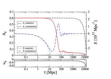
Figure 1: Gauge-invariant energy density perturbation $\Delta_{q}$ and quintessence field fluctuation $X$ as simulated (straight and dashed-dotted lines), compared to the analytic solution of Equations (31) and (98) (dashed and dotted lines) as a function of conformal time $\tau$ for adiabatic initial conditions. Radiation and matter equality corresponds to $\tau=109\rm Mpc$. Shown is the mode for $k=0.1\,\textrm{Mpc}^{-1}$ and the cosmological parameters have been $\Omega_{b}^{0}h^{2}=0.022,\ h=0.7,\ \Omega_{\rm m}^{0}=0.3,\ \Omega_{\rm q}^{0}=0.7$.

Figure 1 demonstrates that the early time behaviour is well described by our analytic formulae. The analytic results agree very well with the simulation for early times, when the mode is outside the horizon. In the lower graph, we plot the equation of state $w_{q}$. The quintessence model used is parameterized by an equation of state $w_{q}(a)=-0.95+0.75(1-a)$, leading to $w_{q}({\rm early})=-0.2$ and according to (98), $X\propto\tau^{0.8}$. This differs from reference Perrotta:1998vf .

We see that including quintessence does not add a new dominant mode. The two additional modes added by the fluctuations of the scalar field are both subdominant and decay with negative eigenvalue $\lambda_{i}$. This is due to the fact that none of the perturbation equations for quintessence equate to zero in the superhorizon limit. This holds for non-tracking quintessence models as well. Let us investigate this in detail. For all the other fluid components, $\Delta_{a}^{\prime}=0$ in the super-horizon limit, but for quintessence we get from eq. (68) that $\Delta_{q}^{\prime}=-3(c_{s(q)}^{2}-w_{q})\Delta_{q}-3w_{q}\Gamma_{q}$. For tracking quintessence, we obtain from equation (85) that $c_{s(q)}^{2}=w_{q}$ and we find

$$\Delta_{q}^{\prime}=-3w_{q}\Gamma_{q}$$ (39)

Since $\Gamma_{q}$ does not vanish except for $w_{q}=1$ (see eq. (84)), this does not equate to zero. Hence, due to the non-vanishing entropy perturbation of quintessence there is no additional dominant mode.

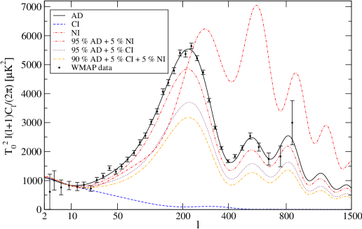
Figure 2: CMB Temperature spectra as a function of multipole $l$ in an early quintessence cosmology. The pure adiabatic (AD), CDM isocurvature (CI), neutrino isocurvature (NI) mode and three different combinations of these dominant modes are plotted. For comparison with experimental data we also give the WMAP measurements of the CMB Spergel:2003cb . The spectrum of the pure baryon isocurvature mode is essentially identical to that of the pure CDM isocurvature mode. All spectra have been normalized to the same power at $l=10$.

IV Isocurvature initial conditions and the CMB

We illustrate the influence of different initial conditions on the CMB with an example. For an analysis of experimental data and a possible isocurvature contribution to the CMB we refer the reader to Enqvist:2000hp ; Trotta:2002iz ; Gordon:2002gv . Here, we merely whish to show the qualitative features of the different modes. We use a modified version of cmbeasy Doran:2003sy ; Seljak:1996is to compute CMB spectra corresponding to different initial conditions for an early quintessence cosmology with parameters as in model A of Caldwell:2003vp . We set the spectral index of the isocurvature modes identical to the spectral index of the pure adiabatic mode, $n_{s}=0.99$. The resulting spectra are plotted in Fig. 2. The spectrum of the pure CDM isocurvature mode decays quickly when going to small scales as has been found in previous works Bucher:2000hy ; Langlois:ar ; Amendola:2001ni . The neutrino isocurvature mode shows prominent peaks at higher multipoles than the adiabatic mode with different peak ratios. For the mixed initial conditions with only small isocurvature contribution, the shape of the curve remains more or less the same. A small admixture of isocurvature fluctuations leads to a decrease of power at larger multipoles if the overall normalization is fixed at $l=10$. Comparison with the WMAP data in the same figure shows that non-adiabatic initial perturbations are strongly constrained. Clearly, pure isocurvature initial conditions are inconsistent with CMB observations.

V Conclusion

We have investigated perturbations in a radiation-dominated universe containing quintessence, CDM, neutrinos, radiation and baryons in the tight coupling limit. The perturbation evolution has been expressed as a differential equation involving a matrix acting on a vector comprised of the perturbation variables. This formulation leads to a systematic determination of the initial conditions. In particular, we find that due to the presence of tracking scalar quintessence no additional dominant mode is introduced. This fact is beautifully transparent in the matrix language. Indeed, contributions of higher order in $x\equiv k\tau$ towards a perturbation vector $\bm{U}$ can easily be determined by solving a simple matrix equation once the constant part of $\bm{U}$ has been determined.

In total, we find four dominant modes and choose them as adiabatic, CDM isocurvature, baryon isocurvature and neutrino isocurvature. For the neutrino isocurvature mode, quintessence automatically is forced to non-adiabaticity. Hence, we could have as well labeled the neutrino isocurvature mode as quintessence isocurvature. To demonstrate the influence on the cosmic microwave background anisotropy spectrum, we have calculated spectra for all modes. Clearly, non-adiabatic contributions are severely constrained by the data. A detailed study may provide ways to put additional constraints on quintessence models or tell us more about the initial perturbations after inflation.

Appendix A Gauge-invariant perturbation equations

In this Appendix we will explain the derivation of equations (2)-(12) in detail.

A.1 The general story

First, we briefly summarize the gauge-invariant approach of Bardeen:kt ; Kodama:bj ; Durrer:2001gq . Perturbing a homogenous Friedman universe, one classifies fluctuations according to their transformation properties with respect to the rotation group. In flat spacetime, we may expand the perturbation variables in terms of harmonic functions york . With $Q_{,i}=\partial Q/\partial x^{i}$ one defines

$$Q_{i}(\bm{k},\bm{x})\equiv-k^{-1}Q(\bm{k},\bm{x})_{,i}$$ (40)

and

$$Q_{ij}(\bm{k},\bm{x})\equiv k^{-2}Q(\bm{k},\bm{x})_{,ij}+\frac{1}{3}\delta_{ij}Q(\bm{k},\bm{x}),$$ (41)

where the $Q(\bm{k},\bm{x})$ are eigenfunctions of the Laplace-operator, $\nabla^{2}Q_{k}(\bm{x})=-k^{2}Q_{k}(\bm{x})$ and in spatially flat universes $Q=\exp(i\bm{k}\bm{x})$. As modes with different $\bm{k}$ decouple in linear theory, we will not display the $\bm{k}$-dependence of $Q$ in the following. The scalar parts of vector and tensor fields can then be written as

$$B_{i}=BQ_{i}$$ (42)

and

$$H_{ij}=H_{L}Q\delta_{ij}+H_{T}Q_{ij}.$$ (43)

respectively.

In this work, we are only interested in scalar fluctuations because scalar quintessence will not influence vector or tensor modes. The most general line element for a perturbed Robertson-Walker metric may be written as

$$\textrm{d}s^{2}=a(\tau)^{2}[-(1+2A)\textrm{d}\tau^{2}-2B_{i}\textrm{d}\tau\textrm{d}x^{i}+$$

$$(\delta_{ij}+2H_{ij})\textrm{d}x^{i}\textrm{d}x^{j}],$$ (44)

where in the scalar case $B_{i}$ and $H_{ij}$ are given by equations (42) and (43). The gauge transformation of a tensor $T$ is given by Bardeen:kt ; Kodama:bj ; Mukhanov:1990me ; Durrer:2001gq ; Doran:2003sy

$$\tilde{T}(x)=T(x)-L_{\epsilon}\bar{T},$$ (45)

where $L_{\epsilon}$ is the Lie derivative. The transformation vector $\epsilon$ can be decomposed as

$$\tilde{\tau}=\tau+T(\tau)Q(\bm{x}),$$ (46)

$$\tilde{x}^{i}=x^{i}+L(\tau)Q^{i}(\bm{x}),$$ (47)

where $L$ and $T$ are arbitrary functions of $\tau$. The transformation properties of the metric perturbations are given by Bardeen:kt ; Doran:2003sy

$$\tilde{A} = A-\mathcal{H}T-\dot{T},$$ (48)

$$\tilde{B} = B+\dot{L}+kT,$$ (49)

$$\tilde{H}_{L} = H_{L}-\mathcal{H}T-\frac{k}{3}L,$$ (50)

$$\tilde{H}_{T} = H_{T}+kL,$$ (51)

where a dot denotes the derivative with respect to conformal time $\tau$ and $\mathcal{H}\equiv\dot{a}(\tau)/a(\tau)$. The functions $L$ and $T$ can be used to eliminate two of the metric perturbations. Popular choices are $A=B=0$ for the synchronous gauge and $B=H_{T}=0$ for the longitudinal gauge.

From equations (48)-(51) one can construct the gauge-invariant Bardeen potentials Bardeen:kt

$$\Psi=A-\mathcal{H}k^{-1}\sigma-k^{-1}\dot{\sigma},$$ (52)

$$\Phi=H_{L}+\frac{1}{3}H_{T}-\mathcal{H}k^{-1}\sigma,$$ (53)

with $\sigma\equiv k^{-1}\dot{H}_{T}-B$. It is worthwhile to note that in longitudinal gauge, for which $B=H_{T}=\sigma=0$, the perturbed metric takes on the simple form

$$ds^{2}_{(long.)}=a(\tau)^{2}\big{[}-(1+2\Psi\,Q)d\tau^{2}\\ +(1+2\Phi\,Q)\delta_{ij}dx^{i}dx^{j}\big{]}.$$ (54)

With ${\rm M}_{\bar{P}}\equiv(8\pi G)^{-1/2}$ denoting the reduced Planck mass, Einstein’s equation reads

$$T^{\mu}_{\;\>\nu}={\rm M}_{\bar{P}}^{2}\left(R^{\mu}_{\;\,\nu}-\frac{1}{2}\delta^{\mu}_{\;\nu}R\right),$$ (55)

where the energy momentum tensor of a perfect fluid is given by

$$T^{\mu}_{\;\>\nu}=p\delta^{\mu}_{\;\nu}+(\rho+p)u^{\mu}u_{\nu}+\pi^{\mu}_{\;\,\nu}.$$ (56)

The covariant 4-velocity is $u_{i}=a(v(\tau)-B)\,Q_{i}$. We define the energy density contrast $\delta$ by $\rho=\bar{\rho}\,(1+\delta(\tau))Q$, the spatial trace by $p\,\delta_{\,j}^{i}=\bar{p}(\tau)(1+\pi_{L}(\tau)Q)\,\delta_{\,j}^{i}$ and the traceless part by $\pi_{\;j}^{i}=\bar{p}\;\Pi\;Q_{\>j}^{i}$. Therefore the components of the energy momentum tensor are

$$T_{\;\;0}^{0} = -\bar{\rho}(1+\delta Q),$$ (57)

$$T^{i}_{\;\;0} = -\bar{\rho}(1+w)\,v\,Q^{i},$$ (58)

$$T^{0}_{\;\;i} = \bar{\rho}\,(1+w)\,(v-B)\,Q_{i},$$ (59)

$$T^{i}_{\;\;j} = \bar{p}\,\left[\left(1+\pi_{L}Q\right)\delta^{i}_{\,j}+\Pi Q^{i}_{\,j}\right].$$ (60)

Given the gauge-transformation properties of $\delta$, $v$ and $\pi_{L}$ Bardeen:kt ; Kodama:bj ; Mukhanov:1990me ; Durrer:2001gq ; Doran:2003sy , one can construct gauge-invariant quantities for the energy density contrast $\Delta$, the velocity $V$ and the entropy perturbation $\Gamma$. These are given by

$$\Delta = \delta+3(1+w)\left(H_{L}+\frac{1}{3}H_{T}\right),$$ (61)

$$V = v-k^{-1}\dot{H}_{T},$$ (62)

$$\Gamma = \pi_{L}-\frac{c_{s}^{2}}{w}\delta.$$ (63)

Here, $c_{s}^{2}\equiv\partial\bar{p}/\partial\bar{\rho}$ is the adiabatic sound speed. From the conservation of the zero component of the energy momentum tensor $\nabla_{\mu}\bar{T}_{\;\;0}^{\mu}=0$ we obtain

$$\frac{\dot{\bar{\rho_{\alpha}}}}{\bar{\rho_{\alpha}}}=-3(1+w_{\alpha})\,\mathcal{H},$$ (64)

where $w=\bar{p}/\bar{\rho}$ is the equation of state of the particular species. The perturbed Einstein equations in gauge-invariant variables are Bardeen:kt ; Kodama:bj ; Mukhanov:1990me ; Durrer:2001gq ; Doran:2003sy :

$$a^{2}\bar{\rho}\Delta = 2\,{\rm M}_{\bar{P}}^{2}\,k^{2}\Phi$$ (65)

$$-3a^{2}\bar{\rho}\,(1+w)\left(\mathcal{H}k^{-1}V-\Phi\right)\!,$$

$$a^{2}(\bar{\rho}+\bar{p})V = 2\,{\rm M}_{\bar{P}}^{2}\,k\left(\mathcal{H}\Psi-\dot{\Phi}\right),$$ (66)

$$a^{2}\bar{p}\,\Pi = -{\rm M}_{\bar{P}}^{2}\,k^{2}(\Phi+\Psi),$$ (67)

In the above, it is understood that the quantities $\Delta,\ V$ and $\Pi$ are the sum of the contributions of all species $\alpha$. Using $\dot{w}=(c_{s}^{2}-w)\dot{\bar{\rho}}/\bar{\rho}$ and (64) we get from $T^{\mu}_{\;\;0;\mu}=0$ that

$$\dot{\Delta}+3(c_{s}^{2}-w)\mathcal{H}\Delta+kV(1+w)+3\mathcal{H}w\Gamma=0,$$ (68)

and from $T^{\mu}_{\;\>i;\mu}=0$

$$\dot{V}=\mathcal{H}(3c_{s}^{2}-1)V+k[\Psi-3c_{s}^{2}\Phi]$$

$$+\frac{c_{s}^{2}k}{1+w}\Delta+\frac{wk}{1+w}\Bigg{[}\Gamma-\frac{2}{3}\Pi\Bigg{]}.$$ (69)

A.2 Gauge-invariant quintessence perturbations

The scalar quintessence field is decomposed into a background and fluctuation part according to $\varphi(\tau,\bm{x})=\bar{\varphi}(\tau)+\chi(\tau,\bm{x})$. The fluctuation can be promoted to a gauge-invariant quantity by defining the gauge-invariant quintessence field fluctuation $X\equiv\chi-\dot{\bar{\varphi}}k^{-1}\sigma$. The field dynamics is governed by the Klein-Gordon equation. For the background, it reads:

$$\ddot{\bar{\varphi}}=-2\mathcal{H}\dot{\bar{\varphi}}-a^{2}V^{\prime}(\varphi),$$ (70)

while the perturbation obeys the equation of motion

$$\ddot{X}=\dot{\bar{\varphi}}(\dot{\Psi}-3\dot{\Phi})-2a^{2}V^{\prime}(\varphi)\Psi\\ -(a^{2}V^{\prime\prime}(\varphi)+k^{2})X-2\mathcal{H}\dot{X}.$$ (71)

Symbol	Meaning	Equation
$\Omega_{\rm species}$	fraction of total energy density	n.a.
$\Omega_{\rm species}^{0}$	fraction of total energy density today	n.a.
$a$	scale factor of the universe	n.a.
$\tau$	conformal time: $\textrm{d}\tau=\textrm{d}t/a$	n.a.
$k$	wavenumber of mode	n.a.
$x$	$k\tau$	n.a.
$\dot{}$	derivative w.r.t conformal time	n.a.
′	derivative w.r.t. $x\frac{\textrm{d}}{\textrm{d}x}$	n.a.
$\mathcal{H}$	$\dot{a}/a$	n.a.
$\Delta$	gauge-inv. density contrast ($\Delta_{g}$ of Kodama:bj )	(61)
$V$	gauge-invariant velocity	(62)
$\Pi$	shear	(60)
$\tilde{V}$	reduced velocity: $\tilde{V}=x^{-1}V$	n.a.
$\tilde{\Pi}$	reduced shear: $\tilde{\Pi}=x^{-2}\Pi$	n.a.

Table 1: Symbols and their meanings.

From the energy momentum tensor for the quintessence field

$$T^{\mu}_{\;\,\nu}=\varphi^{,\mu}\varphi_{,\nu}-\delta^{\mu}_{\;\nu}\left(\frac{1}{2}\varphi^{,\alpha}\varphi_{,\alpha}+V(\varphi)\right),$$ (72)

using $\varphi=\bar{\varphi}+X$ and the longitudinal gauge metric, one gets

$$\delta T^{0\ (lon.)}_{\ 0} = \left[a^{-2}\left(\dot{\bar{\varphi}}^{2}\,\Phi-\dot{X}\dot{\bar{\varphi}}\right)-V^{\prime}(\varphi)X\right]Q$$ (73)

$$\delta T^{i\ (lon.)}_{\ 0} = -a^{-2}\,k\,\dot{\bar{\varphi}}\,X\,Q^{i}.$$ (74)

Using the definition of $\Delta$, equation (61) in longitudinal gauge and $\bar{\rho}_{q}+\bar{p}_{q}=a^{-2}\dot{\bar{\varphi}}^{2}$ one can read off from equation (73) the gauge-invariant expression

$$\Delta_{q}=(1+w_{q})\left[3\Phi-\Psi+\dot{X}\dot{\bar{\varphi}}^{-1}\right]+XV^{\prime}(\varphi)\bar{\rho}_{q}^{(-1)}.$$ (75)

In the same manner, one gets from equation (74) and the fact that $v^{(long.)}=V$ the relation

$$V_{q}=k\dot{\bar{\varphi}}^{-1}X.$$ (76)

Taking the time derivative of equations (75) and (76) and using the equation of motion (71), one obtains the evolution equations

$${\dot{\Delta}}_{q}=(1 + w_{q})\Bigg{[}\frac{2a^{2}V^{\prime}(\varphi)}{\dot{\bar{\varphi}}}\Bigg{(}\frac{\Delta_{q}}{1+w_{q}}-3\Phi\Bigg{)}$$ (77)

$$+ \Bigg{(}\frac{6a\dot{a}V^{\prime}(\varphi)}{k\dot{\bar{\varphi}}}-k\Bigg{)}V_{q}\Bigg{]}+\frac{\dot{w_{q}}\Delta_{q}}{1+w_{q}}$$

and

$${\dot{V}}_{q}=k\left[\frac{\Delta_{q}}{1+w_{q}}-3\Phi+\Psi\right]+2\mathcal{H}V_{q}.$$ (78)

Equation (77) depends on the specific quintessence model through $V^{\prime}$ and $\dot{\bar{\varphi}}$. We can however make progress in the case of nearly constant $w_{q}$: Many quintessence models have solutions for which $\varphi$ approaches an attractor solution irrespectively of its initial value. For these tracking quintessence models Wetterich:fm ; Ratra:1987rm ; Steinhardt:nw , the equation of state of the quintessence field $w_{q}$ is nearly constant during radiation domination. We will use this vanishing of $\dot{w}_{q}$ in the following to derive relations to simplify equation (77). Considering $a^{-2}\dot{\bar{\varphi}}^{2}=(1+w_{q})\rho_{\varphi}$ it follows using the Friedman equation $3a^{-2}{\rm M}_{\bar{P}}^{2}\mathcal{H}^{2}=\rho$ that

$$\dot{\bar{\varphi}}=[3(1+w_{q})\Omega_{q}]^{\frac{1}{2}}{\rm M}_{\bar{P}}\mathcal{H},$$ (79)

and hence

$$\frac{\ddot{\bar{\varphi}}}{\dot{\bar{\varphi}}}=\frac{\textrm{d}}{\textrm{d}\tau}\ln\dot{\bar{\varphi}}=\frac{1}{2}\frac{\dot{\Omega}_{q}}{\Omega_{q}}+\frac{\dot{\mathcal{H}}}{\mathcal{H}},$$ (80)

where we have neglected a term involving $\dot{w}_{q}$. We will in the following assume that at early times, the universe expands as if radiation dominated. In this case, $\mathcal{H}=\tau^{-1}$ and inserting the above equation (80) into the equation of motion (70), one finds

$$\frac{a^{2}V^{\prime}}{\dot{\bar{\varphi}}}=-\frac{3(1-w_{q})}{2\,\tau}.$$ (81)

Using this relation (81), the evolution equation for $\Delta_{q}$ becomes

$${\dot{\Delta}}_{q}=3(w_{q}-1)\frac{k}{x}\bigg{[}\Delta_{q}-3(1+w_{q})\Phi\\ +\left\{3-\frac{x^{2}}{3(w_{q}-1)}\right\}\,(1+w_{q})\tilde{V}_{q}\bigg{]},$$ (82)

whereas the one for the velocity remains almost unaltered while we move to the reduced velocity $\tilde{V}_{q}$:

$$\dot{\tilde{V}}_{q}=\frac{k}{x}\left[\frac{\Delta_{q}}{1+w_{q}}-3\Phi+\Psi\right]+\tau^{-1}\tilde{V}_{q}.$$ (83)

Note that $\Gamma_{q}$ does not usually vanish. Instead, we obtain

$$w_{q}\Gamma_{q}=(1-c_{s(q)}^{2})\left[\Delta_{q}-3(1+w_{q})\Phi+3\frac{\dot{a}}{a}(1+w_{q})\frac{V_{q}}{k}\right]$$ (84)

with the sound speed of quintessence given by

$$c_{s(q)}^{2}=\dot{\overline{p}}_{q}/\dot{\overline{\rho}}_{q}=w_{q}-\frac{1}{3}\frac{a}{\dot{a}}\frac{\dot{w}_{q}}{1+w_{q}}$$ (85)

A.3 Matter and Radiation

Setting $w=c_{s}^{2}=\Gamma=0$ in equations (68) and (A.1), we obtain the cold dark matter evolution equations

$$\dot{\Delta}_{\rm c} = -kx\tilde{V}_{\rm c},$$ (86)

$$\dot{\tilde{V}}_{\rm c} = \frac{k}{x}(-\tilde{V}_{\rm c}+\Psi).$$ (87)

The multipole expansion of the neutrino distribution function Ma:1995ey ; Durrer::fund can be truncated beyond the quadrupole at early times. In terms of density, velocity and shear, it is given by Durrer::fund ; Doran:2003sy

$$\dot{\Delta}_{\nu} = -\frac{4}{3}kx\tilde{V}_{\nu},$$ (88)

$$\dot{\tilde{V}}_{\nu} = \frac{k}{x}\left(\frac{1}{4}\Delta_{\nu}-\tilde{V}_{\nu}-\frac{1}{6}x^{2}\tilde{\Pi}_{\nu}+\Psi-\Phi\right),$$ (89)

$$\dot{\tilde{\Pi}}_{\nu} = \frac{k}{x}\left(\frac{8}{5}\tilde{V}_{\nu}-2\tilde{\Pi}_{\nu}\right).$$ (90)

Deep in the radiation dominated era, for which the initial conditions here are derived, Compton scattering tightly couples photons and baryons Peebles:ag ; Kodama:bj . The coupling leads to $V_{\rm b}=V_{\gamma}$ and the evolution equations become Kodama:bj

$$\dot{\Delta}_{\gamma} = -\frac{4}{3}kx\tilde{V}_{\gamma},$$ (91)

$$\dot{\tilde{V}}_{\gamma} = \frac{k}{x}\left(\frac{1}{4}\Delta_{\gamma}-\tilde{V}_{\gamma}+\Psi-\Phi\right),$$ (92)

$$\dot{\Delta}_{\rm b} = -k\,x\,\tilde{V}_{\gamma}.$$ (93)

As the photon quadrupole and all higher photon multipoles are suppressed during tight coupling, it follows that $\Phi$ is given from Einstein’s equation by

$$\Phi=-\Psi-\Omega_{\nu}\tilde{\Pi}_{\nu},$$ (94)

where we have used the Friedmann equation. Finally, the Poisson equation (65) in terms of the various species is

$$\Psi=-\frac{\sum\limits_{\alpha=c,b,\gamma,\nu,q}\Omega_{\alpha}(\Delta_{\alpha}+3(1+w_{\alpha})\tilde{V}_{\alpha})}{\sum\limits_{\alpha=c,b,\gamma,\nu,q}3(1+w_{\alpha})\Omega_{\alpha}+\frac{2x^{2}}{3}}-\Omega_{\nu}\tilde{\Pi}_{\nu},$$ (95)

where the index $\alpha$ runs over all species. Rewriting the evolution equations (86) - (93) in terms of $\textrm{d}/\textrm{d}\ln x$ and replacing $\Phi$ by means of (94), one arrives at (2)-(11).

Quantity	Scaling behaviour
$\dot{\bar{\varphi}}$	$\propto\tau^{-(1+3w_{q})/2}$
$V^{\prime}$	$\propto\tau^{-(7+3w_{q})/2}$
$V^{\prime\prime}$	$\propto\tau^{-4}$
$\Delta_{q}^{\rm adiab.}$	$const.$
$X_{\rm adiab.}$	$\propto\tau^{(1-3w_{q})/2}$

Table 2: Tracking quintessence in the radiation era: Scaling handbook.

Appendix B Early time quintessence field fluctuations

While throughout this work, we describe quintessence perturbations by the variables $\{\Delta_{q},V_{q}\}$, one could instead use the field fluctuation and its time derivative $\{X,\dot{X}\}$. In this section, we will give analytic expressions for $X$ and $\dot{X}$ in the case of tracking quintessence for super-horizon modes. We will do so assuming that $\Psi$ and $\Phi$ are at least almost constant. As this is not the case for CDM isocurvature and baryon isocurvature, the following steps do not apply in these modes. Furthermore, we will assume that the universe expands as if radiation dominated during the time of interest. In this case, $\mathcal{H}=\tau^{-1}$, $\Omega_{q}\propto\tau^{1-3w_{q}}$ and hence by means of equation (79) $\dot{\bar{\varphi}}\propto\tau^{-\frac{1}{2}(1+3w_{q})}$. Using this, we infer from equation (81) that $V^{\prime}\propto\tau^{-\frac{1}{2}(7+3w_{q})}$. In addition, a straightforward calculation using (80) and (81) yields

$$a^{2}\tau^{2}V^{\prime\prime}=a^{2}\tau^{2}\frac{\textrm{d}V^{\prime}}{\textrm{d}\tau}\frac{\textrm{d}\tau}{\textrm{d}\varphi}=\frac{3}{4}(1-w_{q})(7+3w_{q}).$$ (96)

The equation of motion for $X$ (71) contains a term $\dot{\bar{\varphi}}\left(\dot{\Psi}-3\dot{\Phi}\right)$, which by assumption we may drop. In addition, we see from equation (96), that for super-horizon modes, $a^{2}V^{\prime\prime}\gg k^{2}$ (except for $w_{q}$ very close to $1$), and hence the equation of motion reduces to

$$\ddot{X}=-2a^{2}V^{\prime}\Psi-a^{2}V^{\prime\prime}X-2\frac{\dot{a}}{a}\dot{X}.$$ (97)

Using the power law behaviour in $\tau$ of $V^{\prime},\ V^{\prime\prime}$ and $a$, as well as equations (81) (96), one finds the particular solution

$$X(\tau)=\frac{\tau}{2}\Psi\,\dot{\bar{\varphi}},$$ (98)

as well as two complementary solutions that may be added to obtain the general solution

$$X(\tau)=\frac{\tau}{2}\Psi\,\dot{\bar{\varphi}}+c_{1}\,\tau^{-\frac{1}{2}\left(1-\sqrt{1-4a^{2}\tau^{2}V^{\prime\prime}}\right)}\\ +c_{2}\,\tau^{-\frac{1}{2}\left(1+\sqrt{1-4a^{2}\tau^{2}V^{\prime\prime}}\right)}.$$ (99)

The mode proportional to $c_{2}$ is at least as rapidly decaying as the one proportional to $c_{1}$. Using the explicit form of $4a^{2}\tau^{2}V^{\prime\prime}$, equation (96), we find that $\sqrt{1-4a^{2}\tau^{2}V^{\prime\prime}}$ is imaginary if $w_{q}\in[-\frac{2}{3}(1+\sqrt{6}),-\frac{2}{3}(1-\sqrt{6})]$, which holds for all scalar quintessence models of current interest. Hence, the complementary modes decay $\propto 1/\sqrt{\tau}$ in an oscillating manner.

Coming back to the dominating particular solution (98), Figure 1 shows that the accuracy of this analytic result is indeed high at early times, when compared to numerical simulations.

Inserting the solution (98) and its time derivative into equation (75), we find the simple expression

$$\Delta_{q}=3(1+w_{q})\left(\Phi-\frac{1}{2}\Psi\right),$$ (100)

which is just a restatement of eqn. (23) and (24). Hence, the energy density contrast in tracking quintessence models remains constant on super horizon scales, provided the gravitational potentials are constant to good approximation.

Appendix C Extended Matrix Formulation

For simplicity, we have limited the discussion in section (II.2) to cases where either $w_{q}=1/3$, or quintessence contributions to $A(x)$ are neglected. Here, we will discuss cases for which $w_{q}<1/3$, while the background expands radiation dominated. In this case, $\Omega_{q}\propto\tau^{(1-3w_{q})}$ and we can split the matrix in three parts according to their scaling with $x$:

$$A(x)=A_{0}+x\,A_{1}+x^{(1-3w_{q})}\,A_{q}.$$ (101)

Again, Equation (1) will lead to a solution vector of the form

$$\bm{U}(x)=\bm{U}_{0}+x\,\bm{U}_{1}+x^{(1-3w_{q})}\,\bm{U}_{q}.$$ (102)

Substituting this into Equation (1) and keeping only leading orders in $x$, we get

$$A_{0}\,\bm{U}_{0} = 0,$$ (103)

$$A_{1}\,\bm{U}_{0}+A_{0}\,\bm{U}_{1} = \bm{U}_{1},$$ (104)

$$A_{q}\,\bm{U}_{0}+A_{0}\,\bm{U}_{q} = (1-3w_{q})\,\bm{U}_{q}.$$ (105)

While the conclusion regarding $\bm{U}_{0}$ and $\bm{U}_{1}$ are still the same as in section (II.2), we see that quintessence may introduce a correction

$$\bm{U}_{q}=-\left[A_{0}-(1-3w_{q})\openone\right]^{-1}A_{q}\,\bm{U}_{0}.$$ (106)

This contribution $x^{(1-3w_{q})}\,\bm{U}_{q}$ could in principle dominate over $x\,\bm{U}_{1}$ for $w_{q}>0,\,\Omega_{q}>\Omega_{c}$. However, the contribution is only of interest for the CDM isocurvature and baryon isocurvature modes, as it is otherwise negligible compared to the constant order. Yet for CDM isocurvature and baryon isocurvature, $A_{q}\,\bm{U}_{0}=0$. Therefore, the discussion below applies, leading to $\bm{U}_{q}=0$ for CDM isocurvature and baryon isocurvature modes. One order higher in $x$, there may be a contribution. Yet this is in any case a higher order contribution, which we may neglect.

Finally, we briefly discuss the case of vanishing $\bm{U}_{0}$. This only concerns possible subdominant modes. Equation (104) then yields $A_{0}\,\bm{U}_{1}=\bm{U}_{1}$, i.e. $\bm{U}_{1}$ is an eigenvector of $A_{0}$ with eigenvalue $\lambda=1$. As $A_{0}$ does not have such an eigenvector, we are led to conclude that Equation (1) does not have a regular solution involving $\bm{U}_{1}$, if $\bm{U}_{0}=0$. Turning to Equation (105), we similarly conclude that $\bm{U}_{q}$ needs to be a eigenvector of $A_{0}$ with $\lambda=(1-3w_{q})$ for vanishing $\bm{U}_{0}$. For $w_{q}<1/3$ this is once again excluded and for $w_{q}=1/3$, we just regain the results of section II.2.

References

- [1] D. N. Spergel et al., arXiv:astro-ph/0302209.
- [2] V. F. Mukhanov and G. V. Chibisov, JETP Lett. 33 (1981) 532 [Pisma Zh. Eksp. Teor. Fiz. 33 (1981) 549].
- [3] A. R. Liddle and D. H. Lyth, “Cosmological Inflation And Large-Scale Structure,”
- [4] J. M. Bardeen, P. J. Steinhardt and M. S. Turner, Phys. Rev. D 28, 679 (1983).
- [5] D. H. Lyth, C. Ungarelli and D. Wands, Phys. Rev. D 67 (2003) 023503 [arXiv:astro-ph/0208055].
- [6] N. Bartolo and A. R. Liddle, Phys. Rev. D 65 (2002) 121301 [arXiv:astro-ph/0203076].
- [7] C. P. Ma and E. Bertschinger, Astrophys. J. 455 (1995) 7 [arXiv:astro-ph/9506072].
- [8] C. Wetterich, Nucl. Phys. B 302 (1988) 668.
- [9] B. Ratra and P. J. Peebles, Phys. Rev. D 37 (1988) 3406.
- [10] R. R. Caldwell, R. Dave and P. J. Steinhardt, Phys. Rev. Lett. 80 (1998) 1582 [arXiv:astro-ph/9708069].
- [11] P. T. Viana and A. R. Liddle, Phys. Rev. D 57 (1998) 674 [arXiv:astro-ph/9708247].
- [12] R. Dave, R.R. Caldwell, and P.J. Steinhardt, Phys. Rev. D66, 023516 (2002)
- [13] M. Malquarti and A. R. Liddle, Phys. Rev. D 66 (2002) 123506 [arXiv:astro-ph/0208562].
- [14] L. R. Abramo and F. Finelli, Phys. Rev. D 64 (2001) 083513 [arXiv:astro-ph/0101014].
- [15] M. Kawasaki, T. Moroi and T. Takahashi, Phys. Lett. B 533 (2002) 294 [arXiv:astro-ph/0108081].
- [16] F. Perrotta and C. Baccigalupi, Phys. Rev. D 59 (1999) 123508 [arXiv:astro-ph/9811156].
- [17] R. R. Caldwell, M. Doran, C. M. Mueller, G. Schaefer and C. Wetterich, arXiv:astro-ph/0302505.
- [18] P. J. Steinhardt, L. M. Wang and I. Zlatev, Phys. Rev. D 59 (1999) 123504 [arXiv:astro-ph/9812313].
- [19] J. M. Bardeen, Phys. Rev. D 22 (1980) 1882.
- [20] H. Kodama and M. Sasaki, Prog. Theor. Phys. Suppl. 78 (1984) 1.
- [21] V. F. Mukhanov, H. A. Feldman and R. H. Brandenberger, Phys. Rept. 215 (1992) 203.
- [22] R. Durrer, J. Phys. Stud. 5 (2001) 177 [arXiv:astro-ph/0109522].
- [23] A. K. Rebhan and D. J. Schwarz, Phys. Rev. D 50 (1994) 2541 [arXiv:gr-qc/9403032].
- [24] J. M. Bardeen, Particle Physics and Cosmology, Gordon and Breach, New York, 1989.
- [25] D. Wands, K. A. Malik, D. H. Lyth and A. R. Liddle, Phys. Rev. D 62 (2000) 043527 [arXiv:astro-ph/0003278].
- [26] J. Martin and D. J. Schwarz, Phys. Rev. D 57 (1998) 3302 [arXiv:gr-qc/9704049].
- [27] K. Enqvist, H. Kurki-Suonio and J. Valiviita, Phys. Rev. D 62 (2000) 103003 [arXiv:astro-ph/0006429].
- [28] R. Trotta, A. Riazuelo and R. Durrer, arXiv:astro-ph/0211600.
- [29] C. Gordon and A. Lewis, arXiv:astro-ph/0212248.
- [30] M. Doran, arXiv:astro-ph/0302138.
- [31] U. Seljak and M. Zaldarriaga, Astrophys. J. 469 (1996) 437 [arXiv:astro-ph/9603033].
- [32] M. Bucher, K. Moodley and N. Turok, Phys. Rev. Lett. 87 (2001) 191301 [arXiv:astro-ph/0012141].
- [33] D. Langlois and A. Riazuelo, Phys. Rev. D 62 (2000) 043504 [arXiv:astro-ph/9912497].
- [34] L. Amendola, C. Gordon, D. Wands and M. Sasaki, Phys. Rev. Lett. 88 (2002) 211302 [arXiv:astro-ph/0107089].
- [35] J.W. York, J. Math. Phys. 14 (1973) 456
- [36] R. Durrer, Fund.Cosmic Phys. 15, 209 (1994)
- [37] P. J. Peebles and J. T. Yu, Astrophys. J. 162, 815 (1970).