On the Correlated Spectral and Timing Properties of 4U 1636–53: an Atoll Source at High Accretion Rates

Abstract

We analyze $\sim 600$ ks data from the X-ray observatory Rossi X-ray Timing Explorer of the neutron star low mass X-ray binary and atoll source 4U 1636–53. These observations span almost three years, from April 1996 to February 1999. The color-color and hardness-intensity diagrams show significant secular shifts of the atoll track, similar to what is observed for some Z sources. These are most evident in the hardness-intensity diagram, where shifts in intensity up to $\sim 20\%$ are observed. We find that the intensity shifts in the hardness-intensity diagram are responsible for the parallel tracks observed in the kilohertz quasi periodic oscillations frequency vs. intensity diagram. While the parallel tracks in the frequency vs. color plane partially overlap, systematic long term shifts are still evident. We also study the broad band power spectra of 4U 1636–53 as a function of the source position $S_{\rm a}$ along the track in the color-color diagram. These power spectra are all characteristic of the lower and upper banana state in atoll sources, showing very low frequency noise, band limited noise, and sometimes one or two kHz QPOs. We find that the very low frequency noise in some intervals is not well described by a power law because of an excess of power between 20 and 30 mHz, which can be fitted by a Lorentzian. Also, the characteristic frequency of the band limited noise shows a trend to decrease with increasing $S_{\rm a}$ at high $S_{\rm a}$ values.

1 Introduction

Low Mass X-ray Binaries (LMXB) containing weakly magnetized neutron stars can be divided into two classes based on their correlated X-ray spectral and timing behavior: the so-called Z and atoll sources (Hasinger & van der Klis 1989). Z sources are thus named as they trace out roughly Z-shaped tracks in X-ray color-color or hardness-intensity diagrams on a time scale of hours to days. They are among the most luminous LMXBs, with X-ray luminosities close to the Eddington limit, $L_{\rm Edd}$. Atoll sources sometimes produce patterns which are reminiscent of a ‘C’, have luminosities in the range 0.01–0.5 $L_{\rm Edd}$, and often show X-ray bursts. Their motion in the diagram is slower (on time scales of days to weeks) in the upper left parts of the diagram, the so-called islands, while it is faster (on time scales of hours to a day) in the bottom and right-hand parts of the track, called lower and upper banana, respectively (see e.g. Prins & van der Klis 1997, Méndez et al. 1997, Di Salvo et al. 2001; see also Muno et al. 2002, Gierlinski & Done 2002, van Straaten et al. 2002a, Barret & Olive 2002, for recent work on the behavior of atoll sources in the color-color diagram). In a given source, the islands usually correspond to lower flux levels than the banana branch.

There is evidence that most timing and spectral characteristics of these sources depend in a simple way on the position along the Z or atoll track (see van der Klis 1995, 2000 for reviews). In fact, the characteristic strengths and frequencies of the timing variability of a source usually vary in a monotonic way as the source moves along the track, although some sources can show more complicated behaviors (see, e.g., the case of GX 17+2, Homan et al. 2002). This general and regular behavior suggests that a single parameter, usually proposed to be the mass accretion rate, $\dot{M}$, governs most of this phenomenology; changes in $\dot{M}$ probably cause changes in the accretion flow, which simultaneously affect the X-ray spectrum and the rapid X-ray variability. In this scenario the mass accretion rate is thought to increase from the horizontal branch to the flaring branch in Z sources, and from the islands to the banana branch in atoll sources (see e.g. Hasinger et al. 1990, van der Klis 1995).

At low inferred mass accretion rate the power spectra of these sources are usually dominated by band limited noise (BLN) components. This noise component, usually called in the literature high-frequency noise in atoll sources and low-frequency noise in Z sources, has a flat shape up to a break frequency, $\nu_{\rm break}$, above which it decreases with increasing frequency; it has been often described by a broken power law or a power law with a cutoff at high frequencies. However, since recently, a Lorentzian model for this component is preferred (Olive et al. 1998; Belloni et al. 2002; van Straaten et al. 2002b), since this facilitates the comparison with the power spectra of black hole candidate binaries, which are well fitted by Lorentzians (see e.g. Miyamoto et al. 1991; Nowak 2000), and because a Lorentzian gives sometimes a better description of the noise shape than a broken power law (van Straaten et al. 2002b). Furthermore, Lorentzians are more suitable than power laws to describe components that show large changes in quality factor, which have been observed in some sources (see e.g. Di Salvo et al. 2001; van Straaten et al. 2002b). At high inferred mass accretion rate another type of noise component, with a power-law shape, $P(\nu)\propto\nu^{-\alpha}$ with index $\alpha\sim 1.5-2.0$, called Very Low Frequency Noise (VLFN), dominates at frequencies less than $\sim 1$ Hz. The properties of both these noise components strongly correlate with the position of the source in the color-color diagram. At the lowest inferred $\dot{M}$, the BLN is quite strong (with a fractional rms amplitude of 10–20%). When the mass accretion rate increases, as inferred from the source position in the color-color diagram, the rms amplitude of the BLN decreases to $\leq 2\%$. Simultaneously, the break frequency increases from a few Hz to tens of Hz (this occurs at least in the part of the color-color diagram in which the kHz QPOs are detected; see e.g. Wijnands & van der Klis 1999; Psaltis et al. 1999a, Di Salvo et al. 2001, and references therein). At the highest inferred $\dot{M}$ levels, when the kHz QPOs are no longer detected, a BLN component is sometimes still detected, usually with a characteristic frequency of $10-20$ Hz (e.g. Hasinger & van der Klis 1989, Di Salvo et al. 2001, van Straaten et al. 2002b, see also Sect. 5). The VLFN, on the other hand, usually has its lowest fractional amplitude at low inferred accretion rate ($\leq 1\%$) and its amplitude gradually increases with inferred accretion rate, sometimes up to $\sim 5\%$ (see van der Klis 1995 for a review).

The BLN in atoll and Z sources is usually accompanied by Quasi-Periodic Oscillations (QPOs) at frequencies between 10 and 40 Hz, slightly higher than the break frequency of the BLN. These are the so-called Low-Frequency QPO (LFQPO) in atoll sources, and horizontal branch oscillations (HBO) in Z sources. Similar to the break frequency of the BLN, the frequency of these QPOs increases when the source moves in the color-color diagram in the sense of increasing mass accretion rate (e.g. van der Klis et al. 1985; Stella & Vietri 1998; Ford & van der Klis 1998; van Straaten et al. 2000; Di Salvo et al. 2001; Psaltis et al. 1999a, and references therein). The rms amplitude of the QPOs decreases more or less gradually when the source moves from the horizontal branch to the normal branch in Z sources, and from the islands to the banana in atoll sources.

Observations with the large area instrument on board the Rossi X-ray Timing Explorer (RXTE) led to the discovery in 1996 of QPOs at kilohertz frequencies (kHz QPOs) in the persistent emission of Z and atoll sources. To date, kHz QPOs have been observed in the power spectra of more than 20 LMXBs, with frequencies ranging from a few hundred Hz up to $1200-1300$ Hz (the maximum kHz QPO frequency of 1330 Hz has been measured in 4U 0614+09, van Straaten et al. 2000; see van der Klis 2000 for a review). Usually two kHz QPO peaks (“twin peaks”) are simultaneously observed, the difference between their centroid frequencies being in the range 250–350 Hz. The kHz QPO frequencies increase when the source moves in the color-color diagram in the sense of increasing inferred $\dot{M}$. However, while there is a general correlation between kHz QPO frequencies and position in the color-color diagram, the correlation between kHz QPO frequencies and the source X-ray count rate or X-ray flux in the 2–50 keV energy range is complex; a correlation is observed on short time scales (hours to days), but not on longer time scales. Therefore, when observed at different epochs, in a frequency vs. flux diagram a source produces different tracks that are approximately parallel (e.g. Méndez et al. 1999). A possible explanation of this behavior is that most timing and spectral parameters are determined by the dynamical properties of the accretion disk, while the X-ray flux is determined by the total accretion rate, which may be different from the instantaneous accretion rate through the disk if, for instance, matter can flow radially close to the neutron star (see e.g. van der Klis 2001; note, however, that the radial flow cannot be completely independent of the disk flow, see Méndez et al. 2001). This might also explain the lack of a simple correlation between the X-ray flux (which is usually considered to be a good measure of $\dot{M}$) and other timing properties and/or position in the color-color diagram on time scales of days to weeks (see e.g. Méndez & van der Klis 1999, Ford et al. 2000, and references therein). The whole scenario is not clear yet, and in this paper we will continue to use the widely adopted terminology of “inferred mass accretion rate” to indicate the position of the source in the color-color diagram, keeping in mind that, while this terminology might be correct for the short term (hours to a day), in the longer term there might not be an exact correspondence between instantaneous accretion rate and position in the color-color diagram.

Quasi-coherent oscillations during type-I X-ray bursts have now been detected in several sources, and are all in the rather narrow frequency range between 300 and 600 Hz (see van der Klis 2000; Strohmayer 2001 for reviews). Usually, the frequency of burst oscillations increases by 1–2 Hz during the tail of the burst, and saturates to an “asymptotic frequency” which in a given source is consistent with being constant. This asymptotic frequency is interpreted as the neutron star spin frequency, due to a hot spot (or spots) in an atmospheric layer of the rotating neutron star. For those sources in which both burst oscillations and kHz QPOs have been observed, it has been found that the frequency separation between the two simultaneous kHz QPOs is similar to the frequency of the burst oscillations, or half that value. This suggests a beat frequency mechanism as the origin of the kHz QPOs (Strohmayer et al. 1996; Miller et al. 1998), where the higher-frequency kHz QPO (upper peak) is interpreted as the Keplerian frequency at the innermost edge of the accretion disk, and the lower-frequency kHz QPO (lower peak) is the beat between this Keplerian frequency and the spin frequency, $\nu_{\rm s}$, of the neutron star. However, the peak separation is sometimes significantly smaller than the frequency of the burst oscillations (e.g. Méndez et al. 1998a), and decreases as the frequency of the kHz QPOs increases (van der Klis et al. 1997; Méndez et al. 1998a; Méndez & van der Klis 1999). This led to modifications to the simple beat frequency model (Lamb & Miller 2001), or to different models for the kHz QPOs (see e.g. Stella & Vietri 1999; Osherovich & Titarchuk 1999; Kluźniak & Abramowicz 2002).

4U 1636–536 is one of the most interesting LMXBs of the atoll class. It contains a neutron star accreting matter from a companion star of mass $\sim 0.4$ $M_{\odot}$ with an orbital period of 3.8 hr (see, e.g., van Paradijs et al. 1990). Type-I X-ray bursts were observed several times from this source, sometimes with unusual shapes (e.g. Turner & Breedon 1984; van Paradijs et al. 1986), or unusually long durations (e.g. Wijnands 2001). Duration and temperature of the X-ray bursts in this source strongly correlate with the X-ray spectral and fast variability characteristics of the persistent emission, implying a correlation of all these characteristics with the mass accretion rate or disk dynamical properties (van der Klis et al. 1990). Recently highly coherent oscillations at a frequency of $\sim 582$ Hz have been observed for $\sim 800$ s during a “superburst” from this source (Strohmayer & Markwardt 2002). No evidences of higher harmonics or the subharmonic at 290 Hz have been found. The high coherence of this signal provides further support to a connection between burst oscillations and spin of the neutron star. However, the frequency measured during the superburst is significantly higher than any of the asymptotic burst oscillation frequencies measured for 4U 1636–53 ($\sim 581$ Hz, see e.g. Strohmayer et al. 1998; Giles et al. 2002). Two simultaneous kHz QPOs have been observed in this source, with rms amplitudes increasing with photon energy (Zhang et al. 1996; Wijnands et al. 1997a). The frequency of the lower kHz QPO increases, and its amplitude decreases, with inferred $\dot{M}$, and at high $\dot{M}$ the frequency difference between the two QPOs is in the range $240-280$ Hz, significantly lower than half the frequency of the oscillations detected during type-I bursts (Méndez et al. 1998a). Recently it has been shown that, at low inferred mass accretion rate, the kHz QPO peak separation in 4U 1636–53 is $\sim 323$ Hz, which exceeds the neutron star spin frequency (or half its value) as inferred from burst oscillations (Jonker et al. 2002a).

Third, and possibly fourth, weaker kHz QPOs have been discovered simultaneously with the previously known kHz QPO pair (Jonker et al. 2000); the new kHz QPOs are at frequencies of $\sim 58$ Hz above and below, respectively, the frequency of the lower kHz QPO, suggesting that these are sidebands to the lower kHz QPO. 4U 1636–53, together with 4U 1608–52 and Aql X–1, also shows QPOs at mHz frequencies (Revnivtsev et al. 2001). This feature seems to occur only in a rather narrow range of mass accretion rates, corresponding to X-ray luminosities of $\sim(0.5-1.5)\times 10^{37}$ ergs/s, and they disappear after X-ray bursts. Contrary to the general behavior of QPOs, the rms amplitude of the mHz QPOs strongly decreases with energy.

A systematic study of the correlated rapid X-ray variability and X-ray spectral properties of 4U 1636–53, as derived from color-color and hardness-intensity diagrams, was performed on EXOSAT data by Prins & van der Klis (1997). They found that over a period of two years the source traced out similar patterns in the color-color and hardness-intensity diagrams. However, in observations taken months apart the position of the patterns was slightly (a few percent) shifted in the color-color plane, corresponding to much larger differences in the intensity. They also found that the power spectral components were clearly correlated to the position of the source in this pattern corrected for the shifts due to the secular motion; in particular, with increasing inferred mass accretion rate the fractional rms amplitude of the power-law shaped VLFN increased, while the BLN component amplitude, as well as its cutoff frequency, decreased.

In this paper we present the broad band (0.01-2048 Hz) power spectra of 4U 1636–53 extracted at different positions of the source in the color-color diagram, as well as a study of the secular variations of the position of the atoll pattern in both the hardness-intensity and the color-color diagram.

2 Observations

We analyzed all the observations from the public RXTE archive performed between April 1996 and February 1999. The log of these observations is presented in Table 1. We used data from the Proportional Counter Array (PCA; Zhang et al. 1993) on board RXTE, which consists of five co-aligned Proportional Counter Units (PCU), sensitive in the energy range $2-60$ keV, with a total collecting area of 6250 cm² and a field of view, delimited by collimators, of $1^{\circ}$ FWHM. We selected intervals for which the elevation angle of the source above the Earth limb was greater than 10 degrees. Several bursts occurred during these observations; we excluded those intervals ($\sim 500$ s around each burst) from our analysis. We used the Standard 2 mode data (16 s time resolution) to produce light curves and the color-color diagram, and Event data, with time resolution of 1/8192 s ($\sim 125\mu$s), to produce Fourier power spectra. For the power spectra we also discarded those data ($\sim 8$% of the total) where one or more of the five PCUs were switched off.

Table 1: RXTE observations of 4U 1636–53 used in this paper. The count rate has been normalized to 3 PCA units and is corrected for the background.

Observation	Start Time	Total Time	Averaged Rate
	(UTC)	(sec)	(c/s)
10072-03-03-00	23-04-1996 03:05	1632	1351.16
10072-03-02-00	29-05-1996 01:13	5552	1030.66
10088-01-01-00	27-04-1996 13:45	8928	1040.03
10088-01-04-00	27-04-1996 17:02	3296	1099.83
10088-01-05-00	28-04-1996 12:09	8576	1216.73
10088-01-02-00	29-04-1996 17:37	6256	1043.76
10088-01-03-00	30-04-1996 16:03	6848	1052.10
10088-01-07-01	09-11-1996 20:53	12210	1279.49
10088-01-07-00	14-11-1996 18:12	19790	1802.72
10088-01-07-02	28-12-1996 22:25	13790	1251.22
10088-01-08-00	29-12-1996 03:45	19170	1452.39
10088-01-08-010	29-12-1996 16:32	22670	1286.36
10088-01-08-01	29-12-1996 23:27	10020	1224.70
10088-01-08-02	30-12-1996 03:24	25260	1405.65
10088-01-08-04	31-12-1996 01:09	16380	1396.83
10088-01-08-030	31-12-1996 10:47	25550	1279.06
10088-01-08-03	31-12-1996 18:26	9792	1291.42
10088-01-06-010	05-01-1997 22:05	27390	1310.02
10088-01-06-01	06-01-1997 06:01	3008	1292.10
10088-01-06-07	06-01-1997 08:33	9632	1306.41
10088-01-06-02	07-01-1997 03:28	13500	1674.33
10088-01-06-03	07-01-1997 08:05	12020	1642.56
10088-01-06-04	08-01-1997 04:32	15340	1412.60
10088-01-06-06	08-01-1997 09:37	6448	1434.10
10088-01-06-000	08-01-1997 22:14	21010	2026.24
10088-01-06-00	09-01-1997 04:22	14850	1821.97
10088-01-06-05	09-01-1997 20:37	12210	1701.56
10088-01-06-08	10-01-1997 00:02	18990	1826.38
10088-01-09-00	22-02-1997 06:37	19760	1651.99
10088-01-09-01	23-02-1997 04:49	26270	1865.01
10088-01-09-02	24-02-1997 04:46	20640	1581.61
30053-02-01-000	24-02-1998 23:26	22690	976.50
30053-02-01-001	25-02-1998 05:58	25090	1037.83
30053-02-01-00	25-02-1998 13:15	8464	1187.74
30053-02-02-02	19-08-1998 08:15	15150	1026.38
30053-02-02-01	19-08-1998 13:03	15150	1059.31
30053-02-01-03	19-08-1998 17:50	3648	1059.37
30053-02-01-01	20-08-1998 01:50	1648	1027.12
30053-02-01-02	20-08-1998 03:26	2064	1075.32
30053-02-02-00	20-08-1998 05:11	26110	1241.44
30056-03-01-00	29-12-1998 15:35	3936	1548.72
30056-03-01-03	30-12-1998 14:41	1424	1861.03
30056-03-01-01	30-12-1998 15:34	4032	1854.93
30056-03-01-04	31-12-1998 14:41	1472	1316.05
30056-03-01-02	31-12-1998 15:33	4080	1479.34
40028-01-01-00	12-01-1999 09:28	21500	1521.64
40028-01-02-00	27-02-1999 05:57	4576	1134.68

3 Color-Color and Hardness-Intensity Diagrams

We produced background subtracted lightcurves binned at 16 s using PCA Standard 2 mode data from PCUs 0, 1, and 2, and the PCA background model 2.1b. The lightcurves were divided into four energy bands, $2.0-3.5$, $3.5-6.4$, $6.4-9.7$, $9.7-16.0$ keV (according to the correspondence between fixed energy channels and energy valid for the PCA gain epoch 3). We defined the soft color as the ratio of the count rate in the bands $3.5-6.4$ keV and $2.0-3.5$ keV, the hard color as the ratio of count rate in the bands $9.7-16.0$ keV and $6.4-9.7$ keV, and the intensity as the count rate in the energy band 2–16 keV, in order to produce color-color and hardness-intensity diagrams. The observations considered here span almost three years, from 1996 April 23 to 1999 February 27. All of them fall in the PCA gain epoch 3 (from 1996 April 15 to 1999 March 22). However, to take into account the (smaller) continuous gain changes occurring within one epoch, we used the same procedure already applied in previous works (see e.g. Kuulkers et al. 1994, van Straaten et al. 2000, Di Salvo et al. 2001): we selected RXTE observations of Crab obtained close to the dates of our observations, and calculated the corresponding X-ray colors of Crab. Because the spectrum of Crab is supposed to be constant, any changes observed in the colors of Crab are most probably caused by changes in the instrumental response. Between April 1996 and February 1997 there are no significant shifts in the Crab colors. Between February 1997 and February 1998 the soft and hard colors of Crab increased by $\sim 4$ % and $\sim 2$ %, respectively. From February 1998 to February 1999 the Crab soft color slightly increased by up to $\sim 2.6\%$, while the hard color remained almost constant (changes were less than $\sim 1\%$). To take into account these variations we divided the colors calculated for 4U 1636–53 by the corresponding colors of Crab; these latter were on average: $SC=2.01$ and $HC=0.595$. The changes in the PCA gain, although small, might also affect the source count rate. On average, the Crab count rate decreased from April 1996 to February 1999 by up to $\sim 4.5\%$. So we applied a similar correction to the source intensity, which was normalized to the Crab count rate (the average 2–16 keV Crab count rate was $\sim 2430$ c/s/PCU). The color-color and hardness-intensity diagrams, normalized to the Crab and rebinned so that each point corresponds to 64 s of data, are shown in Fig. 2. We have checked the validity of the correction based on Crab by using spectral fits of 4U 1636–53 observations and the corresponding response matrices (see e.g. Barret & Olive 2002). We find that the correction factors obtained in this way are very similar to those calculated using Crab. They are $\sim 2\%$ larger in soft color and $\sim 0.2\%$ larger in hard color than the Crab-based correction factors, which are comparable with the 1% uncertainty in the PCA response matrix and with the statistical errors on the colors.

                                Figure 1: Color-color diagram (left) and hardness-intensity diagram (right) of 4U 1636–53. Each point represents 64 s of data. The soft and hard colors are defined as the ratio of the count rate in the bands 3.5–6.4 keV/2.0–3.5 keV and 9.7–16 keV/6.4–9.7 keV, respectively. The intensity is defined as the source count rate in the energy band 2–16 keV. The soft and hard colors, as well as the source intensity, are normalized to the Crab values. Note that 1 Crab is $\sim 2.56\times 10^{-9}$ ergs cm^-2 s^-1 keV^-1, corresponding to an average $2-16$ keV count rate of $\sim 2430$ c/s/PCU. Different colors indicate datasets from different observations (P10072: black; P10088: red; P30053: gray; P30056: blue; P40028: light blue; see Table 1). The black curve in the color-color diagram is the spline that we defined to parametrize the position of the source as a function of the coordinate $S_{\rm a}$, and the two big white points indicate the places for which we defined the values $S_{\rm a}=1$ at ($HC=0.99$, $SC=0.71$) and $S_{\rm a}=2$ at ($HC=1.18$, $SC=0.68$), along the spline (see text). The arrows in the hardness-intensity diagram indicate those parts of the diagram where the shifts are particularly evident.                                    
                                    Figure 2: The lower kHz QPO frequency in 4U 1636–53 plotted vs. the 2–16 keV source count rate in Crab units (upper left panel), vs. $S_{\rm a}$ (upper right panel), vs. the hard color (lower left panel) and vs. the soft color (lower right panel). Different colors indicate different datasets; P10088 (from 1996 April 27 to 1996 April 30, red points on the low-flux track), P10072 (1996 May 29, black points), P10088 (from 1996 November 9 to 1997 January 6, red points on the high-flux track), P30053 (1998 February 24–25 and 1998 August 19–20, gray points).

During these observations the source was in the so-called banana state, at high inferred mass accretion rate. As it is apparent from Fig. 2, significant shifts of the position of the atoll track are observed in the hardness-intensity diagram. The most evident shift (indicated by a big arrow in Fig. 2) is between the dataset of observation P10088 (between April 1996 and February 1997, red points) and the dataset of observation P40028 (between January 1999 and February 1999, light-blue points) on the right-hand side of the hardness-intensity diagram, corresponding to the upper banana. Probably a shift is also present within the dataset of observation P10088 (in particular between data obtained before 1996 April 30, which correspond to a lower flux level, and data obtained after 1996 November, which correspond to a higher flux level) and between this latter dataset and the dataset of observations P10072 (in 1996 April and May, black points) and P30053 (in 1998 February and August, gray points) on the left-hand side of the diagram (lower banana, indicated by a small arrow in Fig. 2). In both parts of the hardness-intensity diagram the shift in intensity is $\sim 20\%$. Indeed, it seems that two parallel atoll tracks are present, one shifted $\sim 20\%$ towards lower intensity with respect to the other one. In the color-color diagram, these two atoll tracks overlap each other. However, similar shifts as in the hardness-intensity diagram, although much less evident, are present. This is especially clear in the upper banana (on the right side of the atoll track), where it is possible to see that the points of observation P10088 (red points) have soft color systematically higher than the points of observation P40028 (light-blue points).

To parametrize the position of the source along the atoll track we used the $S$ parametrization method that is usually used for Z sources (introduced by Hasinger et al. 1990; Hertz et al. 1992, and then refined in successive works, see e.g. Homan et al. 2002 and references therein). We projected the points in the color-color diagram onto a spline, $S_{\rm a}$, in which two vertices are placed as reference in the atoll track. We set $S_{\rm a}=1$ at the color-color locus (0.99, 0.71) and $S_{\rm a}=2$ at (1.18, 0.68), as indicated in Fig. 2. A difficulty of this method in the case of atoll sources when compared to Z sources is the lack of sharp corners in the atoll track, which makes the choice of the vertex points rather arbitrary.

4 Study of the Broad Band Power Spectra

4.1 kHz QPOs

One of the aims of this work is to study the timing properties of 4U 1636–53 as a function of the source spectral state, as derived from the position in the color-color diagram. We begin with the study of the kHz QPO frequencies, dividing the PCA lightcurve into 64-s long segments for which we calculated Fourier power spectra up to a Nyquist frequency of 2048 Hz. For each of these segments we measured the average frequency of the kHz QPOs and the position in the color-color diagram using the corresponding value of $S_{\rm a}$. Following Méndez et al. (2001), we produced a dynamic power spectrum for each observation, and we identified those power spectra that showed strong QPOs at frequencies $\ga 250$ Hz. When two QPOs were present in a power spectrum, we selected the one at lower frequency, $\nu_{\rm low}$, which was generally the strongest. We fitted the power spectra with kHz QPOs in the range $\nu_{\rm low}-100$ Hz to $\nu_{\rm low}+100$ Hz, using a function consisting of a constant plus one Lorentzian. In a few of these 64-s segments the QPO was not statistically significant (less than $3\sigma$, single trial). In these cases we averaged several contiguous 64 s segments, but always less than 20, to increase the statistical significance of the detection. We did not combine more than 20 consecutive power spectra to avoid systematic effects (e.g. an artificial broadening) in the measurements due to the variation of the QPO frequencies, which can change by a few tens of Hz within a few hundred seconds. We discarded those data for which this procedure did not reveal any significant kHz QPO. Note, however, that in this way we might also have discarded data with weak QPOs, that are not significantly detected in segments of 1280 s.

In Fig. 2 (left top panel) we plot the frequency of the kHz QPO we measured as a function of the source intensity in the 2–16 keV band (the intensity is in Crab units). We believe that this QPO was always the lower kHz QPO because in our data this was always the strongest one (a comparison between the rms amplitudes of both kHz QPOs is in Fig. 3, top panel). At least two parallel tracks are visible in this figure, demonstrating that there is a complex long-term relation between kHz QPO frequencies and source count rate. Different colors correspond to different dataset; P10088 (from 1996 April 27 to 1996 April 30, corresponding to the red points at the low-flux level), P10072 (data taken in 1996 May 29, black points); P10088 (from 1996 November 9 to 1997 January 6, corresponding to the red points at the high-flux level); P30053 (1998 February 24–25 and 1998 August 19–20, gray points). On long timescales, the source does not move randomly on the kHz frequency versus flux diagram, but jumps back and forth between the same two tracks. Although the observations are not always continuous, we can see that at the beginning of our observing period in April 1996 the source is found at the low flux level, where it remains till the end of May 1996, then it jumps to the high-flux track where it stays from 1996 November 9 to 1997 January 6, and finally the source comes back to the low-flux track where it is found in 1998 February 24–25 and 1998 August 19–20. The difference in intensity between these two tracks is $\sim 20\%$, similar to the intensity shift observed in the hardness-intensity diagram. Indeed the tracks at low and high flux levels correspond, respectively, to the data points at the left-hand ends of the hardness-intensity diagram, where the same $\sim 20\%$ intensity shift is observed.

These two parallel tracks almost overlap each other when we plot the lower peak frequency against the colors (Fig. 2, bottom panels) or $S_{\rm a}$ (Fig. 2, right top panel). However, significant shifts between different observations are still visible in these plots. In particular, datasets corresponding to lower flux levels are found towards the left (closer to the island state) in the color-color diagram (i.e. at lower $S_{\rm a}$ values), while data corresponding to higher flux levels have slightly higher $S_{\rm a}$ values. Similar systematic shifts are also observed in the plots of the kHz QPO frequency versus hard and soft colors, with the source having higher hard colors and lower soft colors at low flux levels, and vice versa (see Fig. 2). The shifts in the QPO frequencies vs. $S_{\rm a}$ diagram are almost certainly due to the fact that we consider a single spline across the color-color diagram, while there are two different atoll tracks corresponding to the two different flux levels. Note however that there is an intrinsic spread in the QPO frequency vs. soft color and vs. $S_{\rm a}$ relations within the dataset P30053 (gray points), although these all show the same flux level and seem to belong to the same atoll track.

Although the data show some scatter, the frequency of the kHz QPO seems to be slightly anticorrelated with the hard color; fitting a line to the hard color vs. frequency relation significantly improves the fit with respect to a constant function; the slope is different from zero at the $\sim 7\sigma$ level for the dataset P10088 (red points), and at the $\sim 4\sigma$ level for the dataset P30053 (gray points). The kHz QPO frequency is slightly correlated with the intensity, whereas there is no significant correlation between the kHz QPO frequency and the soft color or $S_{\rm a}$.

On several occasions we also detected the upper kHz QPO, either directly in the dynamical power spectrum, or in the average power spectrum of an observation. To increase the significance of this QPO and to facilitate measuring its parameters, we needed to average several 64-s power spectra. Because there seems to be no clear correlation between the frequency of the kHz QPOs and $S_{\rm a}$, we used the frequency of the lower kHz QPO to group the power spectra. Following the procedure described in Méndez et al. (1998b), we aligned the individual power spectra according to the frequency of the lower peak, we collected them into groups such that the frequency of this QPO did not vary by more than $15-20$ Hz, and we calculated the average power spectrum for each group. Because we want now to measure the rms amplitudes of the QPOs, here we only used data for which the full energy band was available; based on this requirement we discarded observation P10072, corresponding to $1.2\%$ of the data. (Note that this restriction was not necessary before because then we only measured the QPO frequencies). The measured frequencies, rms amplitudes, and quality factors of both kHz QPOs are plotted in Fig. 3 as a function of the lower peak frequency. The frequency of the lower peak ranges between 780 and 910 Hz. The rms amplitude of the lower peak is approximately constant (or slowly decreasing) up to $\nu_{\rm low}\sim 850$ Hz, and then gradually decreases from $\sim 7\%$ to $\sim 4\%$ while $\nu_{\rm low}$ increases from $\sim 850$ Hz to $\sim 910$ Hz. The upper peak was significantly detected only for $\nu_{\rm low}\ga 840$ Hz. Its frequency increases from $\sim 1100$ to $\sim 1150$ Hz when the frequency of the lower peak increases from $\sim 840$ Hz to $\sim 910$ Hz, while its rms amplitude remains constant around $2.5-3\%$. While the quality factor of the upper kHz QPO is compatible with being constant at a value of $15-20$, the quality factor of the lower kHz QPO significantly decreases from $\sim 200$ to $\sim 50$ with increasing frequency, implying that the lower peak becomes broad at high frequencies. In those intervals in which the upper kHz QPO was not detected with high statistical significance, we calculated the $90\%$ confidence level upper limits on its rms amplitudes, which are still $\sim 3-4\%$ (assuming a frequency separation between the two kHz QPOs of 260 Hz, see below, and a typical quality factor for the upper kHz QPO of 16).

Figure 3: Rms amplitude of the lower kHz QPO (filled triangles, top panel) and the upper kHz QPO (open triangles, top panel), frequency of the upper kHz QPO (middle panel), quality factor, $Q$, of the lower kHz QPO (filled triangles, bottom panel) and of the upper kHz QPO (open triangles, bottom panel) of 4U 1636–53 plotted against the frequency of the lower kHz QPO. For the first four intervals, where the upper kHz QPO was not detected with high statistical significance, we fixed the upper kHz QPO frequency assuming a frequency separation between the two kHz QPOs of 260 Hz, and its quality factor assuming a typical value of 16. We then calculated the 90% confidence level upper limits on its rms amplitude (which are shown in the top panel).

The difference between the frequencies of the kHz QPOs generally decreases from $262.1\pm 9.9$ Hz to $242.4\pm 3.6$ Hz, although the decrease, when compared with the associated uncertainties, is significant only at a $1.8\sigma$ level (an F-test yields a probability in favor of the hypothesis that the frequency difference decreases of $\sim 75\%$). Although the decrease is not highly statistical significant, the trend shown by 4U 1636–53 is in agreement with the trend shown by other sources (see Fig. 4). Also, the frequency separation between the two kHz QPOs is significantly smaller than half the frequency of the quasi-coherent oscillations (the dashed line in Fig. 4) that have been observed in this source during type-I X-ray bursts, in agreement with the results of Méndez et al. (1998a).

Figure 4: The kHz QPO frequency separation as a function of the frequency of the lower peak for Sco X–1 (open triangles, van der Klis et al. 1997), 4U 1608–52 (filled circles, Méndez et al. 1998c), 4U 1728–34 (open circles, Méndez & van der Klis 1999), and 4U 1636–53 (filled triangles, this work). Half the frequency of the burst oscillations, $\nu_{\rm burst}/2\simeq 290$ Hz, for 4U 1636–53 is also shown (dashed line, e.g. Strohmayer et al. 1998).

4.2 Broad band power spectra

To study the time variability of the source over a wide frequency range as a function of the position in the color-color diagram we divided this diagram into several intervals. As already noted in the previous section, some shifts are present in the color-color diagram of all the data combined. In principle we could try to correct for this by drawing two splines, one for each of the two parallel tracks, as it is usually done in the case of Z sources to correct for the secular shifts of the Z track (see e.g. Kuulkers et al. 1994; Jonker et al. 1998; Jonker et al. 2002b). However, in the case of 4U 1636–53 (and of atoll sources in general) this method cannot be applied, because there are no precise vertices in the atoll track, which are instead quite well defined in a Z track. This means that if we draw two splines for the two parallel atoll tracks, the S parametrization along these would be arbitrary, and it would be impossible to compare the $S_{\rm a}$ values corresponding to one track with the other. Another possibility is to use the QPO frequency vs. $S_{\rm a}$ relation to correct for these shifts. As in 4U 1636–53 QPOs are only detected in a small part of the color-color diagram (a small range of $S_{\rm a}$) we cannot use these to correct for the shifts in the color-color diagram or to select the power spectra on the basis of the QPO frequencies. In the following, considering that the shifts in the color-color diagram are much smaller than in the hardness-intensity diagram, we select the power spectra according to their position in the color-color diagram of all the data combined, keeping in mind that they might not correspond exactly to the same position relatively to the atoll track. When possible we analyze separately power spectra corresponding to the same $S_{\rm a}$ value but to different flux levels to see if there are differences between them.

Table 2: Parameters of the very low frequency noise and the band limited noise components.

			VLFN			BLN
Int.	$S_{\rm a}$	Ratea	$\alpha$	rmsb		$\nu_{\rm max}$	$Q$	rms	$\chi^{2}/d.o.f.$	F-testc
Num.		(c/s)		(%)		(Hz)		(%)
1	0.75–1.1	1793.59	$1.386\pm 0.071$	$2.01\pm 0.27$		$69\pm 12$	$0.20\pm 0.15$	$3.70\pm 0.23$	309/136	$1.5\times 10^{-3}$
2	1.1–1.25	2016.86	$1.454\pm 0.027$	$2.458\pm 0.071$		$59.7\pm 3.8$	$0.362\pm 0.072$	$3.27\pm 0.10$	358/137	$2.4\times 10^{-3}$
3	1.25–1.4	2215.07	$1.413\pm 0.020$	$2.742\pm 0.074$		$56.2\pm 3.1$	$0.494\pm 0.078$	$2.994\pm 0.093$	153/137	$1.5\times 10^{-6}$
4	1.4–1.55	2431.22	$1.372\pm 0.046$	$2.81\pm 0.33$		$57\pm 11$	0 (fixed)	$2.70\pm 0.17$	129/137	$2.9\times 10^{-8}$
5	1.55–1.7	2660.44	$1.371\pm 0.087$	$3.62\pm 0.21$		$79\pm 16$	0 (fixed)	$2.59\pm 0.16$	146/137	$3.3\times 10^{-8}$
6	1.7–1.85	2941.12	$1.327\pm 0.021$	$3.81\pm 0.13$		$109\pm 29$	0 (fixed)	$2.41\pm 0.20$	162/138	$1.0\times 10^{-4}$
7	1.85–2	3148.64	$1.345\pm 0.023$	$3.80\pm 0.14$		$46\pm 15$	0 (fixed)	$2.05\pm 0.18$	172/138	$2\times 10^{-8}$
8-low	2–2.2	2626.62	$1.459\pm 0.050$	$4.01\pm 0.24$		$17.9\pm 8.6$	0 (fixed)	$1.72\pm 0.33$	138/140	–
8-high	2–2.2	3382.33	$1.430\pm 0.038$	$3.66\pm 0.23$		$34.1\pm 9.2$	0 (fixed)	$2.04\pm 0.37$	133/137	$4.2\times 10^{-4}$
9-low	2.2–2.45	2693.08	$1.608\pm 0.061$	$4.68\pm 0.37$		$20.7\pm 7.7$	0 (fixed)	$2.41\pm 0.29$	162/140	–
9-high	2.2–2.45	3543.68	$1.422\pm 0.048$	$3.47\pm 0.25$		$24\pm 13$	0 (fixed)	$1.59\pm 0.27$	123/138	$2.7\times 10^{-3}$
10	2.45–3	3332.48	$1.58\pm 0.11$	$4.21\pm 0.79$		$22\pm 12$	$0.31\pm 0.54$	$2.0\pm 0.43$	62/92	–

Errors correspond to $\Delta\chi^{2}=1$.

• PCA count rate, 5 PCUs, not corrected for the background. The background average count rate of the PCA is 132 c/s.

• rms amplitude calculated in the frequency range 0.001–1.0 Hz.

• F-test is the probability of chance improvement of the fit when the very low frequency Lorentzian is included.

Table 3: Parameters of the very low frequency Lorentzian and the kHz QPOs.

	VLF Lor				Lower kHz QPO				Upper kHz QPO
Int.	$\nu_{\rm max}$	$Q$	rms		$\nu_{\rm max}$	$Q$	rms		$\nu_{\rm max}$	$Q$	rms
Num.	(mHz)		(%)		(Hz)		(%)		(Hz)		(%)
1	$25.5\pm 0.38$	$0.40\pm 0.31$	$1.01\pm 0.29$		$864.6\pm 1.2$	$12.49\pm 0.63$	$6.50\pm 0.12$		$1152.8\pm 6.6$	$19.8\pm 6.8$	$2.67\pm 0.28$
2	$28.6\pm 4.6$	0.8 (fixed)	$0.597\pm 0.058$		$866.2\pm 1.4$	$10.23\pm 0.37$	$5.646\pm 0.077$		$1161.2\pm 4.4$	$15.8\pm 2.3$	$2.71\pm 0.15$
3	$25.0\pm 2.6$	0.8 (fixed)	$0.685\pm 0.067$		$901.7\pm 1.5$	$14.6\pm 1.2$	$3.69\pm 0.10$		$1193.0\pm 3.6$	$15.3\pm 2.1$	$2.94\pm 0.14$
4	$23.7\pm 9.5$	$<0.27$	$1.40\pm 0.39$		$911\pm 45$	$3.2\pm 1.3$	$2.92\pm 0.38$		$1227.7\pm 2.7$	$52\pm 14$	$1.69\pm 0.17$
5	$27.8\pm 9.2$	$0.58\pm 0.47$	$1.2^{+1.4}_{-0.24}$		–	–	–		$1233.1\pm 9.0$	$25\pm 15$	$1.31\pm 0.26$
6	$19.2\pm 2.0$	0.8 (fixed)	$1.16\pm 0.13$		–	–	–		–	–	–
7	$23.7\pm 1.8$	0.8 (fixed)	$1.41\pm 0.11$		–	–	–		–	–	–
8-low	25 (fixed)	0.8 (fixed)	$<0.54$		–	–	–		–	–	–
8-high	$27.1\pm 2.9$	0.8 (fixed)	$1.13\pm 0.16$		–	–	–		–	–	–
9-low	25 (fixed)	0.8 (fixed)	$<0.63$		–	–	–		–	–	–
9-high	$29.4\pm 4.9$	0.8 (fixed)	$1.06\pm 0.18$		–	–	–		–	–	–
10	25 (fixed)	0.8 (fixed)	$1.32\pm 0.42$		–	–	–		–	–	–

Errors correspond to $\Delta\chi^{2}=1$, while upper limits to the rms amplitude of the very low frequency Lorentzian correspond to $90\%$ confidence level.

We divided the color-color diagram of 4U 1636–53 into 10 intervals corresponding to different consecutive values of $S_{\rm a}$. We defined the intervals such that we had a sufficient number of them, and enough data in each of them to have good statistics. Each interval contains between 15 and 370 power spectra. For each interval we calculated the average $S_{\rm a}$, using the same spline parametrization described in Sect. 3; the intervals are indicated with numbers from 1 to 10 in order of increasing $S_{\rm a}$. For each interval we computed a power spectrum dividing the PCA light curve into 256-s long segments for which we calculated Fourier power spectra, over the whole PCA energy range, up to a Nyquist frequency of 2048 Hz. We averaged together all power spectra that fell in one interval for more than 40% of the time, weighting each of them by the fraction of the time the source actually spent in the interval. We produced two different power spectra each for intervals 8 and 9, one at a low and one at a high flux level, respectively. For interval 10 the statistics were not enough to produce two separate power spectra, so we preferred to average them together. On average the count rate increases with increasing $S_{\rm a}$ (see Table 2), except for the spectra from intervals 8 and 9 corresponding to lower flux, and for interval 10 (note that in this interval the low and high flux power spectra are averaged together). The high frequency part of each power spectrum ($1200-2048$ Hz, where neither noise nor QPOs are known to be present) was used to estimate the Poisson noise, which was subtracted before fitting the power spectra.

In Fig. 5 we show some representative power spectra (rms-normalized and Poisson-noise subtracted) corresponding to intervals 1, 3, 4, and 6. All of them are typical of the banana state, showing the VLFN, dominating up to frequencies of the order of 0.1 Hz, and a BLN component, dominating up to frequencies of the order of 100 Hz. The power spectra of intervals 1 to 5 also show one or two kHz QPOs. We used a power law, $P(\nu)\propto\nu^{-\alpha}$, to fit the VLFN and Lorentzians to fit the BLN and the kHz QPOs, when present. We fitted the kHz QPOs, when significantly detected, in a limited frequency range (500–2048 Hz) where no other component was present, and using a higher frequency resolution. We then fitted the other components using the full frequency range and fixing the parameters of the kHz QPOs at the values obtained in the high frequency range. This could be done because (as we verified) the frequencies of the kHz QPOs were high enough that they do not affect the parameters of the low frequency features and vice versa.

                    Figure 5: Representative power spectra of 4U 1636–53 corresponding to different intervals in the color-color diagram of Fig. 2; the power units are (rms/mean)²/Hz. Interval numbers are indicated in the top right corners. For each interval, the power spectrum and the best-fit model components are shown; from lower to higher frequencies these components are the very low frequency noise (dashed line), the very low frequency Lorentzian (dashed line), the band limited noise (dotted line), and the kHz QPOs (dot-dashed line and dot-dot-dot-dashed line, respectively, when significantly detected). Note that the parameters for the kHz QPOs were determined using a higher frequency resolution than that used for the broad band power spectra shown here.

The VLFN and the BLN components were present in all the power spectra, while the two kHz QPOs were significantly detected (at more than $3\sigma$) only in the first four intervals. In interval 5 only one kHz QPO is significantly detected, probably the upper kHz QPO given its high frequency ($\sim 1230$ Hz). For some of the intervals these components are not sufficient to give a good fit to the broad band power spectrum. In those cases, some residuals are present between 0.01 and 0.1 Hz due to the VLFN not being well represented by a power law. This is specially apparent in intervals 3 to 5 and 7. We therefore added another Lorentzian to the model, with characteristic frequency $\nu_{\rm max}$ between 20 and 30 mHz. This Lorentzian significantly improved the fit in these intervals. This feature is unlikely to be due to the averaging process, i.e. to the fact that we combine power spectra that may have slightly different characteristic frequencies; in fact we still find it, although at a lower significance level if we divide interval 4 in three subintervals (containing $\sim 10$ power spectra each); sometimes this component is detected in the power spectrum of a single observation. For interval 4 we also tried to fit the complex shape of the VLFN using a broken power law (with a break frequency around 20 mHz) instead of a power law plus a Lorentzian. This model gives a fit of similar quality ($\chi^{2}=133$ for 139 dof) with respect to the power law plus Lorentzian model. In some of the other intervals the addition of this Lorentzian at mHz frequencies was still statistically significant. However, sometimes we could not obtain a stable fit keeping all the parameters free. In those cases, because the goodness of the fit was less sensitive to the quality factor of this Lorentzian than to the other parameters, we fixed $Q$ to a value of 0.8 and let the frequency and the rms amplitude be free. For intervals 8 low-flux, 9 low-flux and 10, the fit was not improved by the addition of this component and we could only find an upper limit to its rms amplitude.

The results of these fits are shown in Tables 2 and 3. The parameters of the Lorentzian components are expressed in terms of the integrated fractional rms amplitude, the quality factor $Q$ ($Q\equiv\nu_{0}/2\Delta$, where $\nu_{0}$ and $\Delta$ are the centroid frequency and the HWHM of the Lorentzian, respectively), and the frequency $\nu_{\rm max}=\nu_{0}\sqrt{1+1/(4Q^{2})}=\sqrt{\nu_{0}^{2}+\Delta^{2}}$ at which the Lorentzian function has its maximum in a $\nu P(\nu)$ representation (Belloni et al. 2002). For narrow features ($Q>1$) $\nu_{\rm max}$ is very close to the centroid frequency $\nu_{0}$, while for Lorentzians with $Q\la 1$, $\nu_{\rm max}$ approaches its HWHM, $\Delta$. We obtained good fits for all the intervals with reduced $\chi^{2}$ ranging from 0.7 to 2.5 for 92 to 140 dof. Some of the $\chi^{2}$ values are rather large, but this is not surprising given the high statistics of the power spectra. Still, for all the intervals the residuals are usually within 2 $\sigma$ and featureless. The largest $\chi^{2}$ values occur for the first two intervals. A careful examination of the residuals shows that the largest contributions to the $\chi^{2}$ come from the region above 500 Hz, and are due to the fact that we fitted the parameters of the kHz QPOs using a higher frequency resolution (these parameters are not therefore the best fit parameters in the broad band and more rebinned power spectra). Note that while the best fit parameters obtained for intervals 8 low-flux and 8 high-flux are compatible with each other (except for the presence of the very low frequency Lorentzian), some (marginal) differences seem to be present between intervals 9 low-flux and 9 high-flux. These differences will be noted below, if necessary. In the following we will describe the results in more detail.

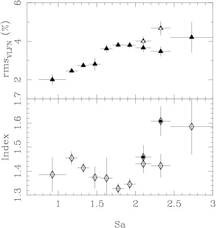
Figure 6: Very low frequency noise (power-law component) rms amplitude (top panel) and power-law index (bottom panel) as a function of $S_{\rm a}$ for 4U 1636–53. The points marked with a white or black dot correspond to the intervals at low flux.

In Fig. 6 we plot the rms amplitude and power-law index of the VLFN as a function of $S_{\rm a}$. While no clear trend is visible in the power-law index, which oscillates around a value of $\sim 1.5$ (probably slightly increasing with $S_{\rm a}$), the VLFN rms amplitude first increases from $2\%$ to $\sim 4\%$ at low values of $S_{\rm a}$, and then saturates at $\sim 4\%$ for $S_{\rm a}$ higher than 1.5. Both the fractional rms amplitude and the power-law index of the VLFN are higher in interval 9 low-flux than in 9 high-flux (the differences are $\sim 2.7\sigma$ and $\sim 2.4\sigma$, respectively). This difference might be due to the presence of an extra component, i.e. the very low frequency Lorentzian, in interval 9 high-flux, which absorbs part of the power. However, looking at the combined rms amplitude of the VLFN and very low frequency Lorentzian (Fig. 7, bottom panel), we can see that the total (very low frequency) rms amplitude of interval 9 low-flux is still higher (at $\sim 2.4\sigma$ confidence level) than that of interval 9 high-flux. On the other hand, no significant differences are visible between intervals 8 low-flux and 8 high-flux. In 4 out of the 10 intervals we significantly detected an excess of power between 0.01 and 0.1 Hz with respect to the power law used to fit the VLFN. We fitted this excess with a (broad) Lorentzian, the parameters of which are shown in Fig. 7 (top and middle panels). The rms amplitude of this feature is between 1% and 1.5% (except for intervals 2 and 3 where it is $\sim 0.6\%$), the quality factor $Q$ is rather low (less than 0.8), and the characteristic frequency, $\nu_{\rm max}$, is between 20 and 30 mHz. The addition of this feature did not significantly improve the fit in intervals 8 low-flux, 9 low-flux and 10. In particular, in intervals 8 low-flux and 9 low-flux, the $90\%$ confidence level upper limits on the very low frequency Lorentzian rms amplitude are $\sim 0.7-0.8\%$, which is significantly lower than the rms amplitudes measured for most of the other intervals.

Figure 7: Very low frequency Lorentzian rms amplitude (top panel) and characteristic frequency (middle panel) as a function of $S_{\rm a}$. The arrows in the top panel indicate the $90\%$ confidence level upper limits calculated for the intervals at low flux. In the bottom panel the total very low frequency rms amplitude (the combined very low frequency Lorentzian and very low frequency noise rms amplitude) is plotted versus $S_{\rm a}$. The points marked with a black dot correspond to the intervals at low flux.

The parameters of the BLN are plotted versus $S_{\rm a}$ in Fig. 8. The rms amplitude (Fig. 8, top panel) decreases from 4% to $\sim 2\%$ with increasing $S_{\rm a}$ up to $S_{\rm a}=2$, and above that value it seems to remain constant at $\sim 2\%$. Again, the rms amplitude for interval 9 low-flux is slightly higher ($\sim 2.1\sigma$) than that for 9 high-flux. The quality factor $Q$ of the BLN (Fig. 8, middle panel) is always less than $\sim 0.5$. Most of the times (intervals 4 to 9) we fixed it to 0 because it could not be determined from the fit, which gave negative values but still compatible with 0. The characteristic frequency $\nu_{\rm max}$ of the BLN (Fig. 8, bottom panel) tends to decrease from $\sim 70$ Hz to $\sim 20$ Hz with increasing $S_{\rm a}$; a linear fit of these points gives a slope of $-24.4\pm 5.8$ Hz per unit $S_{\rm a}$, with a probability of chance improvement with respect to a fit with a constant of $\sim 3.6\times 10^{-3}$. However, in intervals 5 and 6, $\nu_{\rm max}$ seems to increase up to $\sim 100$ Hz (although the uncertainties on these two points are quite large; these points deviate from the linear fit by $\sim 2\sigma$).

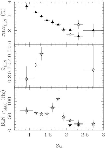
Figure 8: Rms amplitude (top panel), quality factor (middle panel), and characteristic frequency $\nu_{\rm max}$ (bottom panel) of the band limited noise component in 4U 1636–53. The points marked with a white or black dot correspond to the intervals at low flux.

From the broad band spectra we have also measured the parameters of the kHz QPOs as a function of $S_{\rm a}$ for those intervals (from 1 to 5) in which one or two kHz QPOs were detected at more than $3\sigma$ (see Table 3). The frequency of both the kHz QPOs increases with $S_{\rm a}$, as expected. The rms amplitude of the lower kHz QPO decreases from $\sim 6\%$ to $\sim 3\%$ with increasing $S_{\rm a}$. The rms amplitude of the upper kHz QPO slightly increases in intervals 1 to 3 ($S_{\rm a}<1.4$, $\nu_{\rm low}\la 900$ Hz), and then significantly decreases from $\sim 3\%$ to $\sim 1\%$ at higher $S_{\rm a}$ (intervals 4 and 5). The small differences with respect to the kHz QPOs rms amplitudes shown in Fig. 3 are due to the different way in which the power spectra were grouped and averaged together in the two cases. Using the $S_{\rm a}$ values to group the power spectra, we could average together more power spectra; this allows us to see the upper peak up to higher frequencies, but also introduces an artificial broadening of the QPOs due to the fact that their frequencies change with $S_{\rm a}$.

5 Discussion

We have analyzed $\sim 600$ ks of RXTE data of 4U 1636–53 taken between April 1996 and February 1999. We studied the correlated spectral and timing properties of this source using broad band (4 mHz to 2048 Hz) power spectra extracted at different positions of the source in the color-color diagram. The most notable results of this work are: a) The presence of shifts, due to secular motion of the atoll track, in both the hardness-intensity and color-color diagrams; b) The presence of parallel tracks in the kHz QPO frequency versus intensity diagram; for the first time we see that these tracks do not overlap perfectly when plotted versus colors or $S_{\rm a}$; this is probably a consequence of the secular motion of the atoll track mentioned above; c) The deviation of the VLFN-component shape from a pure power law in some of the intervals; d) The characteristic frequency $\nu_{\rm max}$ of the BLN shows a general trend to decrease with increasing $S_{\rm a}$ in the upper banana, i.e. when kHz QPOs are not significantly detected any more. In the following we will discuss these and other results in more detail.

All the observations analyzed here belong to the same PCA gain epoch, PCA gain epoch 3, and therefore only small gain changes are expected. We used Crab observations taken close to the date of our observations to correct the colors and intensity of 4U 1636–53 for these small instrumental effects. The corrected color-color and hardness-intensity diagrams show significant long-term shifts of the atoll track. Secular shifts in both the colors and the intensity in 4U 1636–53 were previously reported by Prins & van der Klis (1997) using EXOSAT observations. We find that the shifts are more evident in the hardness-intensity diagram, where we observe two parallel branches in the upper banana, corresponding to two different intensity levels; it is also possible that the whole atoll track, and not just the upper banana branch, has shifted during the 1999 and part of the 1996 and 1998 observations, which correspond to the low-intensity levels (see Fig. 2). Because the shift at the lower banana (left hand of the diagram) is along the track, we cannot clearly distinguish it from the movement of the source along the track. However, the presence of a shift in this part of the diagram is confirmed by the two-branch distribution of the kHz QPO frequencies versus intensity diagram (see Fig. 2). These shifts are much smaller but still visible in the color-color diagram, where the upper banana branch has significantly moved towards lower soft colors (and probably higher hard colors) during the 1999 observations.

Correlated to the long-term shifts of the atoll track, in the kHz QPO frequency vs. count rate diagram two parallel tracks are observed corresponding to two different flux levels (Fig. 2). During the period of time spanned by our observations, about 2.5 years, 4U 1636–53 is observed to move back and forth (once) between these two tracks; therefore for this source there seem to exist two preferred flux levels at which kHz QPOs are significantly detected. These two tracks tend to overlap each other if we plot the kHz QPO frequency vs. the colors or $S_{\rm a}$, although there are significant offsets still visible in the plots. These offsets are more noticeable in the plot vs. $S_{\rm a}$ or vs. the soft color, whereas they are less evident, although still present, in the plot vs. the hard color. Despite these shifts, the observed behavior is in general consistent with the hypothesis that kHz QPO frequencies depend only on the position of the source in the atoll track, irrespective of the motion of the track as a whole. However, the spread within the dataset P30053 (right hand panels of Fig. 2) indicates that there may be a more complex relation between kHz QPO frequencies and $S_{\rm a}$ or that the spline we chose does not go correctly through all these points. Another possibility is that there are shifts on a timescale of weeks/months of the atoll track in the color-color diagram along the soft color axis (not corresponding to evident intensity shifts, see Fig. 2) that are not clearly seen in the diagram because they occur along the banana branch.

The behavior observed in 4U 1636–53 is similar to the secular motion of the Z-track observed in the Z-sources Cyg X–2 (Kuulkers et al. 1996), GX 5–1 (Kuulkers et al. 1994), GX 340+0 (Kuulkers & van der Klis 1996), and GX 17+2 (Wijnands et al. 1997b; Homan et al. 2002). In these sources shifts in intensity in hardness-intensity diagrams are also reflected in (sometimes) much smaller, but still significant, shifts in the colors in color-color diagrams. These variations have been interpreted in terms of a high inclination angle of these sources, which would allow matter near the equatorial plane to modify the emission from the central region (e.g. Kuulkers et al. 1996). However, as noted by van der Klis (2001), they could also be a consequence of a more general behavior of LMXB accretion, the same behavior that produces the parallel tracks in the kHz QPO frequencies vs. X-ray flux diagram. Indeed, our analysis confirms that secular motion of the atoll track produces the parallel tracks in 4U 1636–53.

As a possible explanation for all this phenomenology, van der Klis (2001) proposed that kHz QPO frequencies, as well as other timing and spectral parameters, to first order depend on the disk inner radius, which is determined by the disk accretion rate normalized by its own long-term average, as could be expected in a radiative disk truncation scenario if luminosity responds, in part, ‘sluggishly’ to disk accretion rate changes. On the other hand, the X-ray luminosity is simply produced by the total accretion rate plus, possibly, nuclear burning. This can be the case if part of the accreted matter escapes from the disk and flows in radially, at a rate that reflects a long term average of the disk accretion rate, and some mechanism (e.g. radiation drag) makes the inner disk radius dependent on the ratio of luminosity to disk accretion rate. In this scenario, the fact that the color-color diagram is also (but less) affected by the jump in the X-ray flux (visible in the hardness-intensity diagram) indicates that the X-ray spectral properties are mainly, but probably not completely, determined by the inner radius of the disk instead of by the total mass accretion rate. In other words, changes in the flux level not affecting the frequencies of the kHz QPOs (i.e. the inner disk radius) may only slightly affect the position in the color-color diagram.

We studied the broad band (4 mHz - 2048 Hz frequency range) power spectra of 4U 1636–53 as a function of the position of the source in the color-color diagram. All power spectra are characteristic of the lower and upper banana states in atoll sources. Only three main components are observed in these power spectra, the VLFN, the BLN, and one or two kHz QPOs. Since there is a shift in the upper part of the banana in the hardness-intensity diagram, due to the $\sim 20\%$ shift of the X-ray flux, for intervals 8 and 9 we extracted two different power spectra corresponding to the two different flux levels. We find that power spectra corresponding to the same position in the color-color diagram but at different flux levels are quite similar to each other. The main difference is in the strength of the very low frequency Lorentzian (Fig. 7), which has an rms amplitude around $1\%$ at high flux level, and less than $\sim 0.7-0.8\%$ at low flux level. A minor difference (if any) is in the fractional rms amplitude of the noise components (Figs. 6 and 8): the rms amplitudes are slightly ($\sim 2-2.7\sigma$) higher for interval 9 low-flux than for 9 high-flux. Note, however, that if we calculate the absolute rms amplitudes (i.e. the fractional rms amplitude multiplied by the flux), these are perfectly compatible between interval 9 low-flux and 9 high-flux.

We observe one or two kHz QPOs only in the lower part of the banana branch, up to $S_{\rm a}\sim 1.7$. For $\nu_{\rm low}\la 840$ Hz the upper peak is not significantly detected, whereas we still detect the lower kHz QPO down to $\sim 780$ Hz. The rms amplitude of the lower peak is approximately constant up to $\nu_{\rm low}\sim 850$ Hz (which is close to the frequency at which the upper peak begins to be significantly detected), and then gradually decreases while $\nu_{\rm low}$ increases. The rms amplitude of the upper peak is consistent with being constant up to $\nu_{\rm low}\sim 900$ Hz, and then it significantly decreases when the lower peak frequency increases further (see Table 2). This is similar to what is observed in other atoll sources (see e.g. Méndez et al. 2001; Di Salvo et al. 2001), where the rms amplitudes of the kHz QPOs remain constant or increase at low frequencies, and decrease at high frequencies. In 4U 1728–34 and 4U 1608–52 the amplitude of the upper kHz QPO decreases monotonically with frequency, whereas the rms amplitude of lower kHz QPO first increases, and then decreases with frequency. In these two sources the rms amplitude of the upper kHz QPO is usually larger than that of the lower kHz QPO. On the contrary, in 4U 1636–53 the rms amplitude of the lower peak is always larger than that of the upper peak (see Fig. 4); this is probably because during these observations the kHz QPOs are at relatively high frequencies, where the lower peak becomes more prominent than the upper peak (cf. Fig. 3a in Di Salvo et al. 2001). Note also that for all these sources (including 4U 1636–53) the rms amplitude of the kHz QPOs is nearly constant in the frequency range in which only one of them is detected.

We have also measured the frequency separation, $\Delta\nu$, between the kHz QPOs, when both of them were present simultaneously. In agreement with Méndez et al. (1998a) we find that $\Delta\nu$ in 4U 1636–53 is always significantly smaller than $290$ Hz, half the frequency of the quasi-coherent oscillations observed during type-I X-ray bursts in this source (see e.g. Strohmayer et al. 1998). This is similar to what has been observed in another atoll source, 4U 1728–34, where $\Delta\nu$ is always significantly smaller than the frequency of the nearly coherent oscillations observed in this source during type-I X-ray bursts, even at the lowest inferred mass accretion rate, when $\Delta\nu$ seems to reach its maximum value (Méndez & van der Klis 1999). In 4U 1636–53, as well as in other similar sources, $\Delta\nu$ decreases as the kHz QPO frequencies increase (van der Klis et al. 1997; Méndez et al. 1998c; Méndez & van der Klis 1999; Ford et al. 1998; Homan et al. 2002; Jonker et al. 2002b; see also Fig. 4). This trend cannot be explained by a simple beat frequency model, since in such model $\Delta\nu$ should be constant and equal to the neutron star spin frequency. Among the different beat frequency models that have been proposed (e.g. Strohmayer et al. 1996; Miller et al. 1998; Campana 2000; Cui 2000), so far only the sonic-point beat frequency model can explain such an offset (Lamb & Miller 2001; see, however, Jonker et al. 2002a). A decrease of the peak separation towards high, as well as towards low, frequencies is also predicted by the relativistic periastron precession model for the kHz QPOs (Stella & Vietri 1999). However, this model shows sometimes severe problems to fit the observed decrease, yielding reasonable fits only when allowing for highly eccentric orbits (Homan et al. 2002). The observational evidence that the kHz QPO frequencies are approximately in a 2:3 frequency ratio led to the model based on parametric resonance between the radial and vertical epicyclic frequencies in a relativistic accretion disk proposed by Kluźniak & Abramowicz 2002 (see also Abramowicz et al. 2002). In this model the difference $\Delta\nu$ is not expected to be constant or equal to the neutron star spin frequency. However, if the kHz QPO frequencies stay in a constant ratio, $\nu_{\rm low}=2/3\;\nu_{\rm high}$, then their difference $\Delta\nu$ should be correlated to the frequencies of the kHz QPOs, and not anticorrelated as is observed. Note, in fact, that there are evidences of a second peak at a value of $\sim 7/9$ in the distribution of the ratio $\nu_{\rm low}/\nu_{\rm high}$ in the case of Sco X–1 (Abramowicz et al. 2002); this high ratio might be due to the fact that the frequency difference decreases at high kHz QPO frequencies.

As in other atoll sources, the rms amplitude of the VLFN increases when the source moves towards the upper banana branch, although in 4U 1636–53 it seems to saturate at high $S_{\rm a}$ values. We found that in some of the intervals the VLFN shows a shape that is more complex than a simple power law, because of the presence of a bump around a frequency between 20 and 30 mHz. We fitted this bump using a Lorentzian, although it could also be due to a change in the slope of the power law describing the VLFN. This feature is not always significantly detected; it seems to be stronger in intervals 4 to 7, with rms amplitudes between 1 and $1.4\%$, while it is much weaker in intervals 2 and 3, where its rms amplitude is $\sim 0.6-0.7\%$. In the intervals at the low-flux level the addition of this feature does not improve the fit, and the $90\%$ upper limits on its rms amplitudes are $\sim 0.7-0.8\%$. Deviations of the VLFN shape from a straight power law were previously observed in some atoll sources; wiggles or bumps at a frequency around 0.1 Hz were particularly evident in the power spectra of the bright atoll sources GX 13+1, GX 9+9, and GX 9+1 (see Hasinger & van der Klis 1989). Note that 4U 1636–53 shows a mHz QPO at a quite stable frequency between 7 and 9 mHz, which is probably associated to some special mode of nuclear burning at the neutron star surface (Revnivtsev et al. 2000; Yu & van der Klis 2002), and there might be a relation between this mHz QPO and the bump observed in the VLFN. Indeed both features show similar rms amplitudes of $\sim 1\%$. However, while the mHz QPO is almost always present, with similar centroid frequencies (even in data separated by years), in the light curve of 4U 1636–53, the VLFN bump is not equally stable in frequency and in rms amplitude. In particular, it does not seem to be present in the intervals at the low-flux level, while it is still detected with statistical significance in the corresponding intervals at high-flux level.

The last feature we want to discuss is the BLN, which is always significantly detected in the power spectra of 4U 1636–53. We fitted it with a Lorentzian, with a low quality factor (always less than 0.5); its rms amplitude generally decreases from $\sim 4\%$ to $\sim 2\%$ with increasing $S_{\rm a}$, in line with the general behavior observed in atoll sources (e.g. Hasinger & van der Klis 1989). In agreement with previous results (Prins & van der Klis 1997), we find that the frequency $\nu_{\rm max}$ of the BLN reaches quite high values, between 50 and 100 Hz, for $S_{\rm a}<1.8$, among the highest ever observed for the BLN (typical values at high inferred accretion rates are 30–60 Hz, e.g. Belloni et al. 2002).

To compare our results on 4U 1636–53 with those obtained for other sources we plotted in Fig. 9 the characteristic frequencies of the features observed in the 4U 1636–53 power spectra (open black symbols), together with those observed in 4U 1728–34 and 4U 0614+09 (filled gray symbols, from van Straaten et al. 2002), versus the frequency of the upper kHz QPO, $\nu_{\rm high}$. In this figure we can distinguish the following features, from the top to the bottom: the lower kHz QPO (squares); the hectohertz QPO, a peaked noise component with a quite constant frequency of $\sim 150$ Hz (stars); the LFQPO (triangles), which weakens at high values of $\nu_{\rm high}$ and disappears for $\nu_{\rm high}\sim 900$ Hz; and the BLN (circles). In 4U 1728–34 this last feature seems to become peaked for $\nu_{\rm high}\ga 900$ Hz: Di Salvo et al. (2001) interpreted these results supposing that the noise component at low inferred accretion rates turns into a QPO at higher accretion rates, while what was called the LFQPO at low accretion rates gradually disappears at higher accretion rates. Therefore in Fig. 9 we marked the characteristic frequencies of this feature at high accretion rates with triangles and we will call it “second LFQPO” (note that the centroid frequency of this feature is approximately, but not exactly, half the frequency of the first LFQPO, so we cannot exclude it is a subharmonic of the first LFQPO). Simultaneously, another noise component appears, with a characteristic frequency of $\sim 7-10$ Hz; these points are marked with circles in Fig. 9.

As can be seen from this figure, the lower kHz QPO in 4U 1636–53 follows the same correlation as that observed for the lower kHz QPO in 4U 1728–34 and 4U 0614+09. The frequency of the BLN in 4U 1636–53 follows a similar correlation to that observed for the LFQPO in 4U 1728–34 and 4U 0614+09. Therefore, on the basis of these correlations, the BLN in 4U 1636–53 can be tentatively identified with the feature that is called second LFQPO in 4U 1728–34 and 4U 0614+09. In the framework of the relativistic precession model, the LFQPO is interpreted as the Lense-Thirring precession frequency of the (slightly tilted) inner parts of the accretion disk, not coaligned with the equatorial plane of the neutron star, around the angular momentum axis of the neutron star (Stella & Vietri 1998); according to the magnetospheric beat-frequency model, this would be the frequency difference between the Keplerian frequency at the magnetospheric radius and the spin frequency of the neutron star (Psaltis et al. 1999b). In both these interpretations, the frequency of this feature is expected to increase with increasing inferred mass accretion rate, i.e. with decreasing inner radius of the disk.

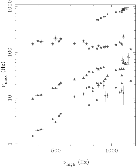
Figure 9: Characteristic frequencies ($\nu_{\rm max}$) of the several Lorentzians used to fit the power spectra of 4U 1728-34, 4U 0614+09 (filled grey symbols, from van Straaten et al. 2001), and 4U 1636–53 (open black symbols, this paper) plotted versus the frequency of the upper kHz QPO. The filled circles mark the Lorentzian identified as the BLN, the filled triangles the Lorentzian identified with the low-frequency QPO, the stars the hectohertz Lorentzian, and the squares the lower kHz QPO. In the case of 4U 1636–53 the frequencies of the band limited noise are in the region where the low-frequency QPO is expected on the basis of the observed correlations, therefore we marked them with open triangles.

However, from the correlation between the BLN frequency and $S_{\rm a}$ in 4U 1636–53 (Fig. 8), we see that $\nu_{\rm max}$ tends to decrease at high values of $S_{\rm a}$ ($S_{\rm a}>1.8$, note that the kHz QPOs in this source disappear for $S_{\rm a}\geq 1.7$). Note, however, that we do not fit any hectohertz QPO in 4U 1636–53 (the addition of this component is not statistically required), and this might affect our measures of the characteristic frequencies of the BLN if the hectohertz QPO is present and not resolved. Indeed time variability seems much weaker in 4U 1636–53 than in 4U 1728–34; a comparison between the power spectra of 4U 1728–34 and 4U 1636–53 at similar kHz QPO frequencies (i.e. for $\nu_{\rm high}\simeq 1150$ Hz) shows that the total rms amplitude is higher in 4U 1728–34 than in 4U 1636–53. However, it is not easy to see whether this is because some of the components are missing in the 4U 1636–53 power spectrum, or all the rms amplitudes are genuinely lower in 4U 1636–53 than in 4U 1728–34. Note that, for $\nu_{\rm high}\simeq 1150$ Hz, 4U 1636–53 and 4U 1728–34 show similar rms amplitudes of the upper and lower kHz QPO (respectively, $2.67\%$ and $6.5\%$ in 4U 1636–53 and $3.68\%$ and $5.59\%$ in 4U 1728–34) and of the VLFN ($2.01\%$ in 4U 1636–53 and $3.39\%$ in 4U 1728–34, cf. Di Salvo et al. 2001). Hence it is possible that some of the time variability components are missing in 4U 1636–53.

Indeed a decrease of the characteristic frequency of the BLN in the upper banana after the disappearance of the kHz QPOs may have been observed in some other similar sources. For instance, in 4U 1820–30 the cutoff frequency of the cutoff power law used to describe the BLN was observed to decrease from $\sim 13.7$ to $\sim 5.5$ Hz along the banana (Wijnands et al. 1999). Further in the banana this noise component evolved first into a broad peaked noise and then into a QPO at a frequency of $\sim 7$ Hz (this behavior is, however, not observed in 4U 1636–53, where this component is always quite broad).

Jumps to lower values in the frequency of the BLN have been observed in 4U 1728–34 and 4U 0614+09 (Ford & van der Klis 1998; van Straaten et al. 2000; Di Salvo et al. 2001; van Straaten et al. 2002b; see also Fig. 9). Also, the noise observed in the upper banana, when the kHz QPOs are no longer detected, is not easily identified in these sources. This is because the power spectra of these sources are very complex (showing several noise components and QPOs) in the island state and lower banana branch, while they become quite simple (showing only VLFN and BLN) in the upper banana; it is not easy therefore to keep track of the evolution of all these components. On the other hand, in the case of 4U 1636–53 the power spectra are much simpler than in other sources already in the lower banana branch, and this allows us to keep track of the evolution of the BLN frequency. If we tentatively identify in 4U 1728–34 and 4U 0614+09 the BLN present in the upper banana with the second LFQPO (as we do in 4U 1636–53), then in 4U 1728–34 at the transition to the upper banana, when the kHz QPOs are no longer detected and the VLFN becomes dominant, the frequency of this feature significantly decreases from $\sim 43$ Hz to $\sim 33$ Hz and then to $\sim 21$ Hz, while in 4U 0614+09 it decreases from $\sim 31$ Hz to $\sim 24$ Hz (van Straaten et al. 2002b; see also van Straaten et al. 2000; Di Salvo et al. 2001). If this interpretation is correct, we can speculate that this feature evolves from a noise component to a QPO and then again to a noise component in 4U 1728–34 and maybe in 4U 0614+09, while it is always quite broad in 4U 1636–53.

A similar behavior may also have been observed in Z sources: a decrease of the HBO frequency with increasing $S_{\rm z}$ was in fact observed with high statistical significance in the Z source GX 17+2, when the kHz QPOs were still present (Wijnands et al. 1996, Homan et al. 2002). In that case, the fundamental frequency of the HBO increases from $\sim 20$ Hz to $\sim 60$ Hz for $S_{\rm z}$ increasing from –0.4 to 1.45, and then it significantly decreases from $\sim 60$ Hz to $\sim 48$ Hz for $S_{\rm z}$ increasing further up to $\sim 2$. This change in the behavior of the HBO frequency occurred when the source was in the Normal Branch, at high inferred mass accretion rates, while simultaneously the frequency of the kHz QPOs, which are thought to track the inner radius of the disk, continued to increase (Homan et al. 2002).

In the framework of the general relativistic precession model this behavior may be explained in terms of the classical precession due to oblateness of the neutron star (Morsink & Stella 1999). However, the relation between the HBO and upper kHz QPO frequencies in GX 17+2 would require rather extreme neutron star parameters: a high neutron star spin frequency (500–700 Hz), a neutron star mass larger than $2M_{\odot}$, and a hard equation of state (see the discussion in Homan et al. 2002). In the framework of the sonic point beat frequency model, this behavior could be explained, for instance, assuming a two-flow model (Wijnands et al. 1996), in which part of the accretion flow is radial outside the magnetosphere (to explain the HBO frequency decrease) and most of the radial flow falls back to the disk before the sonic point is reached (to explain the increase in the kHz QPO frequencies). However, how this should work is not clear, given that the magnetospheric radius and the sonic point radius should be close to each other.

- (1) Abramowicz, M. A., Bulik, T., Bursa, M., & Kluźniak, W. 2002, A&A, submitted (astro-ph/0206490)
- (2) Barret, D., & Olive, J. F., 2002, ApJ, 576, 391
- (3) Belloni, T., Psaltis, D., & van der Klis, M. 2002, ApJ, in press (astro-ph/0202213)
- (4) Campana, S. 2000, ApJ, 534, L79
- (5) Cui, W. 2000, ApJ, 534, L, 31
- (6) Di Salvo, T., Méndez, M., van der Klis, M., Ford, E., & Robba, N. R. 2001, ApJ, 546, 1107
- (7) Ford, E. C., van der Klis, M., Méndez, M., et al. 2000, ApJ, 537, 368
- (8) Ford, E., & van der Klis, M. 1998, ApJ, 506, L39
- (9) Gierlinski, M., & Done, C. 2002, MNRAS, 331, L47
- (10) Giles, A. B., Hill, K. M., Strohmayer, T. E., & Cummings, N. 2002, ApJ, 568, 222
- (11) Hasinger, G., & van der Klis, M. 1989, A&A, 225, 79
- (12) Hasinger, G., van der Klis, M., Ebisawa, K., Dotani, T., & Mitsuda, K. 1990, A&A, 235, 131
- (13) Hertz, P., Vaughan, B., Wood, K. S., et al. 1992, ApJ, 396, 201
- (14) Homan, J., van der Klis, M., Jonker, P.G., et al. 2002, ApJ, 568, 878
- (15) Jonker, P. G., Wijnands, R., van der Klis, M., et al. 1998, ApJ, 499, L191
- (16) Jonker, P. G., Méndez, M., & van der Klis, M. 2000, ApJ, 540, L29
- (17) Jonker, P. G., Méndez, M., & van der Klis, M. 2002a, MNRAS, 336, L1
- (18) Jonker, P. G., van der Klis, M., Homan, J., et al. 2002b, MNRAS, 333, 665
- (19) Kluźniak, W., & Abramowicz, M. A. 2002, A&A, submitted (astro-ph/0203314)
- (20) Kuulkers, E., van der Klis, M., Oosterbroek, T., et al. 1994, A&A, 289, 795
- (21) Kuulkers, E., van der Klis, M., & Vaughan, B. A. 1996, A&A, 311, 197
- (22) Kuulkers, E. & van der Klis, M. 1996, A&A, 314, 567
- (23) Lamb, F. K., & Miller, M. C. 2001, ApJ, 554, 1210
- (24) Méndez, M., van der Klis, M., van Paradijs, J., et al. 1997, ApJ, 485, L37
- (25) Méndez, M., van der Klis, M., & van Paradijs, J. 1998a, ApJ, 506, L117
- (26) Méndez, M., van der Klis, M., van Paradijs, J., et al. 1998b, ApJ, 494, L65
- (27) Méndez, M., van der Klis, M., Wijnands, R., et al. 1998c, ApJ, 505, L23
- (28) Méndez, M., & van der Klis, M. 1999, ApJ, 517, L51
- (29) Méndez, M., van der Klis, M., Ford, E. C., Wijnands, R., & van Paradijs, J. 1999, ApJ, 511, L49
- (30) Méndez, M., van der Klis, M., & Ford, E. C. 2001, ApJ, 561, 1016
- (31) Miller, M. C., Lamb, F. K., & Psaltis, D. 1998, ApJ, 508, 791
- (32) Miyamoto, S., Kimura, K., Kitamoto, S., Dotani, T., & Ebisawa, K. 1991, ApJ, 383, 784
- (33) Morsink, S. M., & Stella, L. 1999, ApJ, 513, 827
- (34) Muno, M. P., Remillard, R. A., & Chakrabarty, D. 2002, ApJ, 568, L35
- (35) Nowak, M. A. 2000, MNRAS, 318, 361
- (36) Olive, J. F., Barret, D., Boirin, L., et al. 1998, A&A 333, 942
- (37) Osherovich, V., & Titarchuk, L. 1999, ApJ, 522, L113
- (38) Prins, S., & van der Klis, M. 1997, A&A, 319, 498
- (39) Psaltis, D., Belloni, T., & van der Klis, M. 1999a, ApJ, 520, 262
- (40) Psaltis, D., Wijnands, R., Homan, J. et al. 1999b, ApJ, 520, 763
- (41) Revnivtsev, M., Churazov, E., Gilfanov, M., & Sunyaev, R. 2001, A&A, 372, 138
- (42) Stella, L., & Vietri, M. 1998, ApJ, 492, L59
- (43) Stella, L., & Vietri, M. 1999, Phys. Rev., 82, L17
- (44) Strohmayer, T. E., Zhang, W., Swank, J. H., White, N. E., & Lapidus, I. 1998, ApJ, 498, L135
- (45) Strohmayer, T. E. 2001, in Astrophysical Sources of Gravitational Radiation for Ground-Based Detectors (astro-ph/0101160)
- (46) Strohmayer, T. E., Zhang, W., Swank, J. H., et al. 1996, ApJ, 469, L9
- (47) Strohmayer, T. E., & Markwardt, C. B., 2002, ApJ, 577, 337
- (48) Turner, M. J. L., & Breedon, L. M. 1984, MNRAS, 208, 29
- (49) van der Klis, M. 2001, ApJ, 561, 943
- (50) van der Klis, M. 1995, in X-Ray Binaries, Lewin W. H. G., van Paradijs J., van den Heuvel E. P. J. eds., Cambridge Astrophysics Series, Cambridge
- (51) van der Klis, M. 2000, ARA&A, 38, 717
- (52) van der Klis, M., Hasinger, G., Damen, E., et al. 1990, ApJ, 360, L19
- (53) van der Klis, M., Wijnands, R. A. D., Horne, K., & Chen, W. 1997, ApJ, 481, L97
- (54) van der Klis, M., Jansen, F., van Paradijs, J., et al. 1985, Nature, 316, 225
- (55) van Paradijs, J., van der Klis, M., van Amerongen, S., et al. 1990, A&A, 234, 181
- (56) van Paradijs, J., Sztajno, M., Lewin, W. H. G., et al. 1986, MNRAS, 221, 617
- (57) van Straaten, S., van der Klis, M., & Méndez, M., 2002a, in preparation
- (58) van Straaten, S., van der Klis, M., Di Salvo, T., & Belloni, T. 2002b, ApJ, 568, 912
- (59) van Straaten, S., Ford, E. C., van der Klis, M., Méndez, M., & Kaaret, P. 2000, ApJ, 540, 1049
- (60) Wijnands, R., & van der Klis, M. 1999, ApJ, 514, 939
- (61) Wijnands, R., van der Klis, M., & Rijkhorst, E. J. 1999, ApJ, 512, L39
- (62) Wijnands, R. 2001, ApJ, 554, L59
- (63) Wijnands, R. A. D., van der Klis, M., van Paradijs, J., et al. 1997a, ApJ, 479, L141
- (64) Wijnands, R., Homan, J., van der Klis, M., et al. 1997b, ApJ, 490, L157
- (65) Wijnands, R., van der Klis, M., Psaltis, D., et al. 1996, ApJ, 469, L5
- (66) Yu, W., & van der Klis, M. 2002, ApJ, 567, L67
- (67) Zhang, W., Giles, A. B., Jahoda, K., et al. 1993, Proc. SPIE, 2006, 324
- (68) Zhang, W., Lapidus, I., White, N. E., & Titarchuk, L. 1996, ApJ, 473, L135