The effect of signal digitisation in CMB experiments

Signal digitisation may produce significant effects in balloon - borne or space CMB experiments, when the limited bandwidth for downlink of data requires for loss-less data compression. In fact, the data compressibilty depends on the quantisation step $q$ applied on board by the instrument acquisition chain. In this paper we present a study of the impact of the quantization error in CMB experiments using, as a working case, simulated data from the Planck/LFI 30 and 100 GHz channels. At TOD level, the effect of the quantization can be approximated as a source of nearly normally distributed noise, with RMS $\simeq q/\sqrt{12N_{\mathrm{s}}}$, with deviations from normality becoming relevant for a relatively small number of repeated measures $N_{\mathrm{s}}\mbox{$\stackrel{{{}_{<}}}{{{}_{\sim}}}$}20$. At map level, the data quantization alters the noise distribution and the expectation of some higher order moments. We find a constant ratio, $\simeq 1/({\sqrt{12}\sigma/q})$, between the RMS of the quantization noise and RMS of the instrumental noise, $\sigma$ over the map ($\simeq 0.14$ for $\sigma/q\simeq 2$), while, for $\sigma/q\sim 2$, the bias on the expectation for higher order moments is comparable to their sampling variances. Finally, we find that the quantization introduces a power excess, $C_{\ell}^{ex}$, that, although related to the instrument and mission parameters, is weakly dependent on the multipole $\ell$ at middle and large $\ell$ and can be quite accurately subtracted. For $\sigma/q\simeq 2$, the residual uncertainty, $\Delta C_{\ell}^{ex}$, implied by this subtraction is of only $\simeq$1–2$\%$ of the RMS uncertainty, $\Delta C_{\ell}^{noise}$, on $C_{\ell}^{sky}$ reconstruction due to the noise power, $C_{\ell}^{noise}$. Only for $\ell\mbox{$\stackrel{{{}_{<}}}{{{}_{\sim}}}$}30$ the quantization removal is less accurate; in fact, the $1/f$ noise features, although efficiently removed, increase $C_{\ell}^{noise}$, $\Delta C_{\ell}^{noise}$, $C_{\ell}^{ex}$ and then $\Delta C_{\ell}^{ex}$; anyway, at low multipoles $C_{\ell}^{\rm sky}\gg\Delta C_{\ell}^{\rm noise}>\Delta C_{\ell}^{ex}$. This work is based on Planck LFI activities.

1 Introduction

Since the successful detection of CMB anisotropy at angular scales $\theta\mbox{$\stackrel{{{}_{>}}}{{{}_{\sim}}}$}7^{\circ}$ by the $COBE$-DMR experiment (Smoot et al. 1992; Bennet et al.1996; Górski et al. 1996), a large number of detections on smaller angular scales with increased sensitivity by both ground-based and balloon-borne experiments have followed (e.g. Lasenby et al. 1998, De Bernardis & Masi 1998, Bersanelli & Maino & Mennella 2002 for reviews). Recent exciting results from BOOMERanG (De Bernardis et al. 2000), MAXIMA-1 (Balbi et al. 2000), DASI (Pryke et al. 2001) and CBI experiments (Mason et al. 2001) have provided strong support to the inflationary scenario for structure formation and a universe with $\Omega_{0}\sim 1$. However to fully extract the wealth of cosmological information encoded in the CMB angular power spectrum, extreme mapping sensitivity is required. Only space missions can provide the proper combination of full-sky view and low level of systematic effects that is necessary for “precision” CMB measurements (Danese et al. 1996), as demonstrated by the excellent results from the NASA satellite MAP  (Bennett et al. 2003). The ESA satellite Planck  (Mandolesi et al. 1998; Puget et al. 1998) is designed to measure the CMB anisotropy with an accuracy mainly set by astrophysical limits on a wide frequency range (30–900 GHz) and with unprecedent angular resolution and sensitivity.

While space experiments benefit from unique environmental conditions, numerous technical issues need to be addressed. One of them is the limited bandwidth for downloading of data to the Earth which often imposes strong limits on the available telemetry rate. For this reason it is often necessary to use loss less compression methods (Maris et al. 2000a) in order to reduce the data rate. Because the efficiency compression algorithms depends on the quantization step applied to the observed signal by the instrument acquisition chain on board the satellite, it is necessary to find the optimal trade-off between the required compression rate and the quantisation step, which needs not to be too high to preserve the scientific quality of the measured data.

If the quantization step, $q$, is significantly smaller than the signal root mean square (RMS), $\sigma_{\mathrm{T}}$, and no saturation of the quantization levels occurs then the distortion induced by the signal quantization can be well approximated by an additive source of non-Gaussian white noise with variance $\approx q^{2}/12$ (Kollar, 1994). Corrections to this simplified model are required when $\sigma_{\mathrm{T}}/q\mbox{$\stackrel{{{}_{<}}}{{{}_{\sim}}}$}1$, which depend on the kind of the total signal in input to the quantization stage of the on-board acquisition chain (Kollar 1994). For example, in the case of a pure white noise signal they are exponentially damped by a factor $\exp[-2(\pi\sigma_{\mathrm{T}}/q)^{2}]$. On the contrary, in the case of a sinusoidal signal (e.g. like the CMB dipole), corrections may by quite large and no simple analytical expressions can be written.

It is worth noting that, in general, the observing strategy implies repeated observations of the same region of the sky on different time scales with detectors operating at different frequencies. Therefore, considering that a sample is the result of the average of $N$ repeated observations, we have that for a normally distributed signal with $\sigma_{\mathrm{T}}/q\gg 1$ the RMS of the quantization noise, $\sigma_{q}$ is:

$$\sigma_{q}\approx\frac{q}{\sqrt{12N}}\,.$$ (1)

In CMB experiments, however, the approximations of normal distributed signal and low $\sigma/q$ are often not strictly applicable. In fact the astrophysical signal is in general not normally distributed, and it is often required to use large quantization steps (i.e. $\sigma_{\mathrm{T}}/q\sim 1$). The instrumental noise power spectrum usually shows a $1/f^{\alpha}$ spectral behaviour, with $\alpha\sim 1-2$ (see Burigana et al. 1997a and Seiffert et al. 2002), while the number of samples is not uniformly distributed when projected onto a sky map. Therefore it is apparent that the validity of eq. (1) needs to be assessed in the context of space CMB experiments in order to evaluate possible deviations from this simple formula.

In this paper we evaluate the impact of the quantization error on CMB measurements from space and provide tools and methods to optimize the quantization step to reach the required compression rate with minimal impact on the scientific output.

We show examples relative to the Planck/LFI 30 and 100 GHz channels. However, the formalism, tools and methods developed here are general and applicable to CMB anisotropy experiment based on differential receivers, as well as to other kinds of experiments with large quantization steps.

Using Monte Carlo simulations we estimate the effect of software quantization on the data considering various quantization functions and for different values of the quantization step. We also discuss the impact of different experimental conditions like the total number of repeated measures for sample, $N_{s}$, the white noise RMS, $\sigma$, the $1/f^{\alpha}$ noise and the scanning strategy. The impact of quantization is evaluated at three different levels: on time ordered data, on sky maps and their statistical moments, and on the angular power spectrum.

In Sect. 2 we describe the analytical model of signal quantization and discuss the adopted numerical approach. Sect. 3 describes our results in terms of effects on TOD and maps including their statistical properties, and on the angular power spectrum. In Sect. 4 we present the possibility to reduce the effect of quantization in the recovered power spectrum. Finally, we discuss our main results and draw the conclusions in section 5. To improve readability, some mathematical details are reported in Appendix A while in Appendix B we briefly verify that the extra-quantitazion step introduced via hardware by the analog to digital converter (ADC) quantization represents a minor effect with respect to the subsequent software quantization extensively discussed in the paper. In Appendix C we report on statistical moments of the map adopted in the simulations and of several foregrounds, for comparison.

2 Analytical model and numerical simulations

2.1 Analytical model

During a typical CMB experiment from space, the measured signal is first digitized and compressed on board and subsequently reconstructed on ground. Furthermore the scanning strategy usually involves multiple measurements from the same pointing direction that are subsequently averaged during ground data analysis. Therefore in order to assess the impact of the quantization error we need to consider the complete process, from quantization, to reconstruction and averaging. In the following of this paper this process will be referred to as “QRA process”.

Let us neglect the data compression step (that is out of the scope of our paper) and consider first the on-board quantization. In general the instrument output will be constituted by a Time Ordered Data stream (TOD) representing the sky temperature anisotropy; in the case of differential receivers, for example, the TOD will contain consecutive samples of temperature differences (sky minus reference signal) so that the $i^{th}$ sample, $\Delta T_{i}$, will be quantized as (Maris et al. 2000a ):

$$\mbox{$\Delta T_{i}^{\mathrm{Q}}$}=\mbox{$\mathcal{Q}$}\left[\frac{\mbox{$\Delta T_{i}$}-\mbox{$\Delta T_{\star}$}}{q}\right]\,,$$ (2)

where $\mbox{$\mathcal{Q}$}[x]$ and $\Delta T_{\star}$ represent the quantization operator and a zero level.

The second step is the data reconstruction, i.e. the inverse of eq. (2). This second step is necessary because both the quantization step $q$ and the offset $\Delta T_{\star}$ will not necessarily be constant during the mission; this implies that eq. (2) needs to be inverted in order to be able to compare measurements obtained in different periods of observation. The data reconstruction step can be defined as:

$$\mbox{$\Delta T_{i}^{\mathrm{R}}$}=\left(\mbox{$\Delta T_{i}^{\mathrm{Q}}$}+\mbox{$\mathcal{O}_{\wr}$}\right)\cdot q+\mbox{$\Delta T_{\star}$}$$ (3)

where $\mathcal{O}_{\wr}$ is an offset that depends on the considered quantization operator, and is defined by:

$$\mbox{$\mathcal{O}_{\wr}$}=\mbox{$\mathrm{E}$}[\mbox{$\Delta T_{i}$}]/q-\mbox{$\mathrm{E}$}[\mbox{$\Delta T_{i}^{\mathrm{Q}}$}]$$ (4)

where $\mbox{$\mathrm{E}$}[X]$ represents the expectation of the random variable $X$.

The value of $\mathcal{O}_{\wr}$ is dependent on the quantization operator and assumes the values of $0$, $+1/2$, $-1/2$ for the $\mbox{$\mathrm{floor}$}(x)$, $\mbox{$\mathrm{ceil}$}(x)$ or $\mbox{$\mathrm{round}$}(x)$ operators, respectively. In the case of the $\mbox{$\mathrm{trunc}$}(x)$ operator the offset depends on the statistics of the random variable $X$; if $X>0$ then $\mbox{$\mathrm{trunc}$}(x)\equiv\mbox{$\mathrm{floor}$}(x)$, if $X<0$, $\mbox{$\mathrm{trunc}$}(x)\equiv\mbox{$\mathrm{ceil}$}(x)$.

In our analytical treatment we will neglect the presence of an offset; its effect will be discussed in the next section. Other simplifying assumptions are that the signal is quantized in equally spaced steps and that $\Delta T_{\star}$ is always $>0$. With simple considerations we can estimate the effect of the QRA process on the reconstructed maps and power spectra. We consider the case of typical CMB anisotropy experiments consisting of collections of many TODs each one based on the averaging over $N_{\mathrm{s}}$ repetitions of the observation of the same stripe in the sky .

Assuming that the QRA acts mainly as an added white noise source, the effect of quantization on the power spectrum can be easily estimated. Let $C_{\ell,\mbox{$N_{\mathrm{s}}$}}^{wn}$ the white-noise induced excess of power and $C_{\ell,\mbox{$N_{\mathrm{s}}$}}^{\mathrm{QRA}}$ the equivalent excess of power induced by the QRA process; then we have that $\mbox{$C_{\ell,\mbox{$N_{\mathrm{s}}$}}^{wn}$}=\mbox{$K_{\mathrm{wn}}^{2}$}\,\sigma^{2}/\mbox{$N_{\mathrm{s}}$}$ and $\mbox{$C_{\ell,\mbox{$N_{\mathrm{s}}$}}^{\mathrm{QRA}}$}=\mbox{$K_{\mathrm{qra}}^{2}$}\,q^{2}/(12\,\mbox{$N_{\mathrm{s}}$})$, where $N_{\mathrm{s}}$ represents the number of times that each pixel in the sky is measured during a single stripe and the pixel dependent normalization constants $K_{\mathrm{wn}}^{2}$ and $K_{\mathrm{qra}}^{2}$ are determined by the scanning strategy (and the processing of the data, assumed to be a linear process). Since both quantized and not-quantized signals are sampled and processed in the same way, in principle we expect $\mbox{$K_{\mathrm{wn}}^{2}$}=\mbox{$K_{\mathrm{qra}}^{2}$}$. Therefore, for any $N_{\mathrm{s}}$ we have:

$$\frac{\mbox{$C_{\ell,N}^{wn}$}}{\mbox{$C_{\ell,N}^{\mathrm{QRA}}$}}=\left(\sqrt{12}\,\frac{\sigma}{q}\right)^{2}\,.$$ (5)

The total noise power spectrum after quantization can be well approximated by:

$$C_{\ell,N}^{total}=\mbox{$C_{\ell,N}^{wn}$}\left[1+\left(\sqrt{12}\,\frac{\sigma}{q}\right)^{-2}\right]\,.$$ (6)

For $\sigma/q\simeq 2$ (as in the case of the Planck baseline) the noise power excess will be increased by $\simeq 2$%. A similar relation holds for the ratio between the variance of the quantization noise and the variance of the white noise in a map:

$$\sigma_{\mathrm{map},\,\mathrm{total}}^{2}=\sigma_{\mathrm{map},\,\mathrm{wn}}^{2}\left[1+\left(\sqrt{12}\frac{\sigma}{q}\right)^{-2}\right],$$ (7)

where $\sigma_{\mathrm{map},\,\mathrm{wn}}$ is the RMS white noise in the map introduced by the instrument. This formula holds both for the noise average variance on the map and for the noise variance of a given pixel in the map.

2.2 Numerical simulations

The analytical model described in the previous section allows a simple, first-order estimation of the QRA effect. We have performed numerical simulations to verify and quantify the validity and the accuracy of the analytical model and to study effects (like the presence of the skysignal and $1/f^{\alpha}$ noise) not accounted for in the analytical approach. The simulations are representative of the Planck mission. In particular we consider here the 30 GHz and 100 GHz channels of Planck/LFI assuming angular resolutions of $\simeq 33^{\prime}$ and $10^{\prime}$, respectively.

2.2.1 Simulation tools

To evaluate the effect of QRA process through numerical simulations we have $a)$ simulated the data acquisition during the space mission (with and without signal QRA processing) producing TODs; $b)$ produced reconstructed sky maps and power spectra from simulated TODs; $c)$ compared the results when including or not the QRA process.

The simulation of the data acquisition during the mission has been performed using the Planck Flight Simulator developed by Burigana et al. (1997b ). In this code we have included numerical tools to simulate data acquisition, signal quantization and signal reconstruction to allow the parallel generation of a quantized data stream plus a data stream of reconstructed data and to perform the statistical evaluation of the quantization error at TOD level (Maris et al. 2000b ).

The Flight Simulator is a code that simulates the CMB measurement according to the Planck satellite scanning strategy. Planck is a spinner (with the telescope observing axis nearly perpendicular to its spin axis) that will map the sky through a large set of near great circles at a spin rate of 1 r.p.m. The satellite will orbit around the Lagrangian point L2 of the Sun-Earth system maintaining the spin-axis always in the anti-Sun direction. The measurement strategy is to acquire data from the same sky circle for about one hour before repointing the spin axis by approximately $2.5^{\prime}$, so that the same sky pixel is measured $\sim 60$ times in each scan circle.

The main simplifying assumptions concerning the scanning strategy that we have considered in our simulations are: (i) no drift or variation in the spin rate (equal to 1 r.p.m. for all the simulation), (ii) instantaneous repointing, (iii) perfect pointing with $85^{\circ}$ observing angle with respect to the spin axis.

The only astrophysical signal considered in the simulation has been a map describing the CMB fluctuations, therefore neglecting the effect of the dipole and of the galactic and extragalactic contributions. To the astrophysical signal we have also added white noise representative of the 30 GHz and 100 GHz radiometers (with an RMS of 1.056 mK and 3.325 mK, respectively, corresponding to integration times of 0.03 s and 0.009 s). In some simulations we also added a 1/$f$ component to study the effect of correlated noise on quantization; to this aim we considered two cases, with a 1/$f$ component having a knee frequency of 0.1 and 0.5 Hz, respectively. The first is representative of a typical worst case expected in LFI radiometers (for which we require a knee frequency $\leq 0.05$ Hz) while the second has been studied to enhance any possible effect connected to 1/$f$ noise but is clearly non representative of expected performances.

The code developed by Burigana et al. (1997b ) and Maino et al. (Maino:destriping (1999)) has been used to generate maps from TODs. With this code it is also possible to significantly reduce correlated systematic effects as the $1/f^{\alpha}$ noise stripes from the data before generating the final maps. Power spectra have been obtained from the generated maps using the anafast code of the HEALPix package from Górsky et al. 1998, adopted here to pixelize the sky.

2.2.2 Numerical procedures

Let us now consider the time ordered data stream produced by the Flight Simulator as an ordered sequence of measured temperature differences $\Delta T_{i}$, as in eq. (2). If we now take into account that for each pointing direction in the sky, indicated by the subscript $p$, on a given stripe (i.e., a scan circle for Planck) there will be $N_{\mathrm{s}}$ repeated measurements then we can reorder the TOD according to two indices, $(s,p)$, the first one ($s=1,\dots,\mbox{$N_{\mathrm{s}}$}$) representing the repeated pixel measurements and the second one representing the pointing direction. Therefore we will have that $\Delta T_{i}\equiv\mbox{$\Delta T$}_{s,p}$ ($i\leftrightarrow(s,p)$).

Now for a single sample $(s,p)$ the quantization error introduced by a quantization step, $q$, can be defined as:

$$\mbox{$\Delta T_{s,p}^{\mathrm{E}}$}=\mbox{$\Delta T_{s,p}^{\mathrm{R}}$}-\mbox{$\Delta T$}_{s,p}\,,$$ (8)

where the superscript $R$ indicates a sample that has been quantized and then reconstructed. In a similar way we can define the following quantities averaged over $N_{\mathrm{s}}$ multiple measurements for each direction, $p$, in the sky:

$$\mbox{$\Delta T$}_{p}=\frac{1}{\mbox{$N_{\mathrm{s}}$}}\Sigma_{s}\Delta T_{s,p},$$ (9)

$$\mbox{$\Delta T$}_{p}^{R}=\frac{1}{\mbox{$N_{\mathrm{s}}$}}\Sigma_{s}\mbox{$\Delta T_{s,p}^{\mathrm{R}}$},$$ (10)

$$\mbox{$\Delta T$}_{p}^{E}=\mbox{$\Delta T$}_{p}^{R}-\mbox{$\Delta T$}_{p}=\frac{1}{\mbox{$N_{\mathrm{s}}$}}\Sigma_{s}\mbox{$\Delta T_{s,p}^{\mathrm{E}}$}\,.$$ (11)

To characterize the quantization error for the LFI signal at TOD level we study the behavior of the distribution moments of $\mbox{$\Delta T$}_{p}$, $\mbox{$\Delta T$}^{R}_{p}$ and $\mbox{$\Delta T$}_{p}^{E}$. In particular we analyze their expectation, RMS, skewness and kurtosis as a function of the quantization step $q$, of the quantization function $\mbox{$\mathcal{Q}$}[\cdot]$ and of the number of samples $N_{\mathrm{s}}$.

The time ordered data with and without quantization have then be used to produce maps and power spectra in order to study the quantization error at these other two levels.

The simulations have been carried out considering three distinct quantization steps, i.e. $q\approx 0.5$, 1.0, 2.0 mK for the 30 GHz channel and $q\approx 1.2$, 2.4, 4.9 mK for the 100 GHz channel. These three values of $q$ correspond, for each frequency channel, to $\sigma/q\simeq 2$, 1 and 1/2, respectively. The case $\sigma/q\simeq 2$ corresponds to the current Planck baseline; the case $\sigma/q\sim 1/2$ is representative of a case in which the noise model for the quantization distortion is expected to fail, while the intermediate case was chosen evaluate possible deviations of the dependence of the quantization error on $\sigma/q$ from a power law.

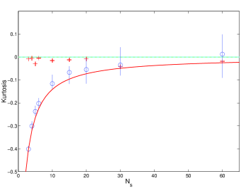
Figure 1: Kurtosis for the distribution of the random errors for the QRA process as a function of $N_{\mathrm{s}}$. Crosses represents the kurtosis for the original simulated samples without quantization and reconstruction, but just averaging them in groups of $N_{\mathrm{s}}$. Bars represents the distribution of values of kurtosis for the quantization error for the averages of $N_{\mathrm{s}}$ quantized and reconstructed simulated samples. Note that the realisation of simulated TOD is not changed when $q$ is changed so that the variability is just due to the QRA process. Circles represent the averaged kurtosis for the points forming the bar. The solid line represents the theoretical expectation for the kurtosis after $N_{\mathrm{s}}$ averages.

3 Results

In this section we discuss the effect of signal quantization at the three different levels of time ordered data, final maps and power spectra. The results presented in this section have been produced considering the quantization operator $\mbox{$\mathrm{floor}$}(x)$; this assumption can be made without any loss of generality, as all the quantization operators can be considered equivalent provided that the proper offset is applied in the reconstruction formula, eq. 3.

3.1 Effect of quantization at TOD level

To study the effect of quantization at the level of the time-ordered data stream we focus on the statistical properties of the data-stream by evaluating the various moments of the statistical distribution of the quantization error.

3.1.1 Mean value of the quantization error distribution

The first statistical quantity that we have analyzed is the mean value of the quantization error to evaluate if the QRA process introduces any spurious bias in the data and how this varies with $q$. This is relevant in the context of space missions, in which possible variations in the noise properties of the detectors will require slight modifications in time of $q$ in order to maintain constant the $\sigma/q$ ratio required for optimal compression. Therefore if any bias in the data is introduced by quantization it is reasonable to expect that this bias will vary in time (because of the changes in $q$) leading to systematic errors in the final maps and power spectra.

We have calculated the mean value of the quantization error ($\mbox{$\Delta T_{60}^{\mathrm{E}}$}=\mbox{$\mathrm{mean}$}[\mbox{$\Delta T_{60,p}^{\mathrm{E}}$}]$, see eq. 11) for a $\sim$ 1 year-long data stream, considering different values of the quantization step $q$. Our results show that quantization introduces a bias in the data at a level $|\mbox{$\Delta T_{60}^{\mathrm{E}}$}|/q<10^{-3}$ which implies $|\mbox{$\Delta T_{60}^{\mathrm{E}}$}|<2$ $\mu$K even for the largest values of $q$. This offset effect is small, and in addition it can be efficiently removed by destriping algorithms.

Therefore we can expect systematic effects in the time ordered data at a very low level and the time scales of the updating of $q$ on board ($>$ 24 hours). Furthermore these effects can be efficiently reduced by applying destriping and/or map-making methods to the time-ordered data and therefore they do not represent a concern.

3.1.2 RMS of the quantization error distribution

The rms of the quatization error can be easily evaluated from the theoretical eq. (1). The validity of this relationship has been checked numerically by calculating the rms of the quantization error (indicated by $S_{N}$) for several TODs generated with various values of $q$ and $N$ around the reference values $N_{\mathrm{0}}=60$ and $\mbox{$q_{\mathrm{0}}$}=0.305$ mK/adu, equivalent to $\sigma/q=3.462$ for the 30 GHz channel and $\sigma/q=10.902$ for the 100 GHz channel. A fit of $S_{N}$ with the relation:

$$\ln S_{N}=\ln\Sigma_{0}+m_{\mathrm{N}}\ln(\mbox{$N_{\mathrm{s}}$}/N_{\mathrm{0}})+m_{\mathrm{q}}\ln(q/\mbox{$q_{\mathrm{0}}$})\,.$$ (12)

yielded $\Sigma_{0}\approx\mbox{$q_{\mathrm{0}}$}/\sqrt{12N_{0}}$, $m_{\mathrm{N}}\approx-1/2$ and $m_{\mathrm{q}}\approx 1$ with an accuracy up to the third decimal figure. This confirms that in our case eq. (1) is a very good approximation of the rms value of the quantization error distribution.

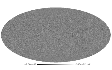
Figure 2: The upper frame is the map of the quantization error after the QRA process, plus destriping and map making, for a single 30 GHz radiometer, with $\sigma=1.053$ mK, $\sigma/q\approx 2$, $\mbox{$f_{\mathrm{knee}}$}=0.1$ Hz, $\mbox{$N_{\mathrm{s}}$}=60$. The lower frame is the ratio of the histogram of the map divided by the histogram of a random variable normally distributed. The zero line represents the case of a quantization error normally distributed. The y-scale represents the $\log_{1}0$ of the ratio. As indicated even in Tab. 1 the quantization error is not completely normal distributed. However the largest deviations are for large quantization errors, in excess of twice the RMS of the QRA process.

3.1.3 Higher moments of the quantization error distribution

In the ideal case of a normally distributed random signal with $\sigma/q\gg 1$ the QRA error will also be nearly normally distributed and the indices of skewness and kurtosis  are expected to vanish. On the other hand if $\sigma/q$ approaches 1 then it is reasonable to expect a change in the values of the higher moments of the statistical distribution for the QRA error.

From theory, the effect on higher moments may be evaluated from the characteristic function for the distribution of the sampled values after QRA processing $\Theta\Pi^{\mathrm{QRA}}_{N_{\mathrm{s}}}(\omega)=\Phi_{N_{\mathrm{s}}}(\omega)\Pi_{N_{\mathrm{s}}}(\omega)$, where $\omega$ is a real variable, $\Phi_{N_{\mathrm{s}}}(\omega)$ is the characteristic function for the QRA process (see appendix A), $\Pi_{N_{\mathrm{s}}}(\omega)$ is the corresponding function for the averaged input data. The expectation for central moments of order $k\geq 0$ being $\mu_{k}=(-i)^{k}d^{k}\Theta\Pi^{\mathrm{QRA}}_{N_{\mathrm{s}}}(\omega)/d\omega^{k}|_{\omega=0}$. Since the QRA error is even distributed around zero expectations for its moments for $k$ odd are null. If the same is true for the distribution of the unprocessed data then the expectations for all the $\mu_{k}$ with $k$ odd is null. The same does not hold for the expectation of moments with $k$ even, in this case the QRA process may introduce a not null bias for some or all of them. In addition the QRA process randomly scatters about their expectation both odd and even moments. Then QRA process randomly changes the measured value of moments of any order $k$ for a given realization respect to the values which have been measured in the case of no-QRA. Higher order moments, at least up to the fourth order, are needed to full-characterize the statistical properties of the QRA error. However the complete study of these features is beyond the scope of this work and we limit our investigation to few cases illustrative of the methods which may be applied to study them and the kind of perturbation which may be expected on real data. We may attempt a deeper investigation of this effect as numerical tools will improve enough to allow the generation and the analysis of a large data set of simulated missions.

To evaluate the departure of the averaged quantization error from a normal distribution we have calculated the skewness and the kurtosis for the distribution of $\mbox{$\Delta T$}_{p}$, $\mbox{$\Delta T$}_{p}^{R}$ and $\mbox{$\Delta T$}_{p}^{E}$ for various values of $q$ and $N_{\mathrm{s}}$.

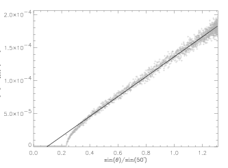
Figure 3: Colatitudinal distribution of the variance of the QRA error on a sky map for $\sigma/q\approx 2$ and the 100 GHz channel. The straight line represents the best linear fit.

As expected, the QRA process alters the sampling skewness in the input signal, so that it has meaning to put:

$$\frac{\Delta\mbox{$\mathrm{Skewness}$}}{\mbox{$\mathrm{Skewness}$}[\mbox{$\Delta T$}_{p}]}=\frac{(\mbox{$\mathrm{Skewness}$}[\mbox{$\Delta T$}_{p}^{R}]-\mbox{$\mathrm{Skewness}$}[\mbox{$\Delta T$}_{p}])}{\mbox{$\mathrm{Skewness}$}[\mbox{$\Delta T$}_{p}]}\neq 0\,.$$

In our simulation we observe values of $|\Delta\mbox{$\mathrm{Skewness}$}/\mbox{$\mathrm{Skewness}$}[\mbox{$\Delta T$}_{p}]|$ up to $50\%$ at the TOD level, comparable to the random fluctuations induced by the sampling variance. It is worth noting that this value depends on $N_{s}$ so that the variation in skewness decreases with increasing the number of samples of the same data point and that on the final map (in which each pixel will be the result of averaging a large number of measurement, especially close to the ecliptic poles) the impact on the skewness of the CMB distribution is even smaller (see Table 2) and varying with the colatitude.

In Fig. 1 we show the behavior of the kurtosis for the QRA error ($\mbox{$\mathrm{E}$}[\mbox{$\mathrm{Kurtosis}$}[\mbox{$\Delta T$}_{p}^{\mathrm{E}}]]$) as a function of $N_{\mathrm{s}}$. From the plot it is apparent that the expectation of the kurtosis goes to zero for increasing values of $N_{\mathrm{s}}$. For an input signal with small expected kurtosis, the value of the sampling kurtosis at TOD level can be changed by the QRA process by a factor up to $\sim 2$, again comparable with the sampling variance for the kurtosis in our TODs. As for the skewness the impact on the kurtosis on maps is even smaller. However it is important to recall that, while skewness is changed randomly by the QLA, i.e. no bias is added by QRA to the skewness estimator, the same does not hold for the kurtosis. For the kurtosis, the bias is $-3/[1+12(\sigma/q)^{2}]^{2}$, equivalent to $\simeq-0.001$ for $\sigma/q\simeq 2$. However, once the quantization step and the scanning strategy is defined, it is a simple matter to calculate this bias and to remove it.

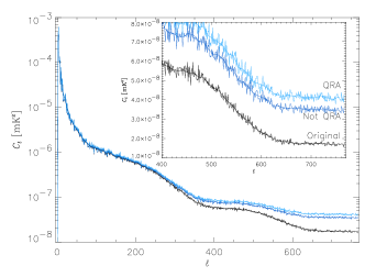
Figure 4: Power Spectra from maps for simulated CMB, simulated CMB plus noise, simulated CMB plus noise plus QRA processing (labelled as Original, Not QRA, QRA) for the 30 GHz channel (1 radiometer). The inset is an enlargement of the power spectra for $l>400$. For each power spectrum a smoothed spectrum is overlapped to the original spectrum. The $\sigma/q\approx 0.5$ values has been chosen to increase the quantization effect. In the nominal case $\sigma/q\approx 2$ the effect is about 16 times smaller and difficult to see in the plot.

A non-zero value of the kurtosis in the distribution of the QRA error changes the statistical significance of the confidence limits respect to the usual definition of “standard error” for which “$1\sigma$ corresponds to a 68.27% confidence level”. To recover the standard error definition we have scaled the variance of the quantization error by a multiplicative factor $\alpha_{N_{\mathrm{s}}}\mbox{$\stackrel{{{}_{>}}}{{{}_{\sim}}}$}1$, which decreases monotonically for increasing $N_{\mathrm{s}}$, whose $\lim_{N_{\mathrm{s}}\rightarrow\infty}\alpha_{N_{\mathrm{s}}}=1$, and $\alpha_{1}=1.18$. Appendix A describes the computation of $\alpha_{N_{\mathrm{s}}}$.

These results allow to safely apply the usual error propagation to combine both signal plus noise and the QRA error with an accuracy better than some $\mu$K. The $1\sigma$ confidence level for a given temperature average, $\mu_{N_{\mathrm{s}}}$ may be expressed as:

$$\mu_{N_{\mathrm{s}}}\pm\sigma_{N_{\mathrm{s}}}\pm\alpha_{N_{\mathrm{s}}}\sigma_{q,N_{\mathrm{s}}}\approx\mu_{N_{\mathrm{s}}}\pm\sqrt{\sigma_{N_{\mathrm{s}}}^{2}+\alpha_{N_{\mathrm{s}}}^{2}\sigma_{q,N_{\mathrm{s}}}^{2}}\,.$$ (13)

The first term down the square root represents the effect of the white-noise, while the second term the effect of the QRA error. Note that since the $\alpha_{N}$ correction equations (6) and (7) are valid only for $N_{\mathrm{s}}$ sufficiently large to have $|\alpha_{N_{\mathrm{s}}}-1|\ll 1$. Otherwise the $\left(\sqrt{12}{\sigma}/{q}\right)^{-2}$ has to be scaled by $\alpha_{N_{\mathrm{s}}}^{2}$ in eq. (6) and eq. (7). In the case of Planck-LFI the measurement redundancy ($\mbox{$N_{\mathrm{s}}$}\sim 60$) is such that the distributions of the QRA error is sufficiently well approximated by a normal distribution to apply the usual formula for the error propagation.

Figure 5: Power excess induced by signal quantization for the 30 GHz channel, 1 radiometer, i.e. the power spectrum for the quantization error map (panel a)) reported also in terms of $\delta T_{\ell}=(C_{\ell}\ell(2\ell+1)/4\pi)^{1/2}$ (panel b)). Ratio between the power excess induced by the QRA process and the power spectrum of the unquantized map (noise plus sky) (panel c)) and its square root (panel d)). The approximate value of $\sigma/q$ for each curve is reported in panel a) (see Tab. 1 for the corresponding exact values).

3.2 Effect on the reconstructed map

30 GHz
$\sigma/q$	% variance increase	% variance increase	a	b
	(from simulations)	(from eq. 7)	(mK2)	(mK2)
2.076	1.94	1.93	$(-9.00\pm 1.16)\times 10^{-7}$	$(2.105\pm 0.011)\times 10^{-5}$
1.038	7.67	7.73	$(-4.02\pm 0.46)\times 10^{-6}$	$(8.459\pm 0.046)\times 10^{-5}$
0.519	30.94	30.59	$(-1.30\pm 0.19)\times 10^{-6}$	$(3.399\pm 0.019)\times 10^{-4}$
100 GHz
$\sigma/q$	% variance increase	% variance increase	a	b
	(from simulations)	(from eq. 7)	(mK2)	(mK2)
2.724	1.13	1.12	$(-1.436\pm 0.036)\times 10^{-5}$	$(1.5061\pm 0.0036)\times 10^{-4}$
1.362	4.55	4.49	$(-5.903\pm 0.146)\times 10^{-5}$	$(6.0464\pm 0.0145)\times 10^{-4}$
0.681	17.57	17.97	$(-2.241\pm 0.056)\times 10^{-4}$	$(2.3698\pm 0.0055)\times 10^{-3}$

Table 1: Quantization error at map level. The table compares the % variance increase determined by simulations ($\left(\sigma_{\mathrm{map},\,\mathrm{total}}^{2}/\sigma_{\mathrm{map},\,\mathrm{wn}}^{2}-1\right)\times 100$) with the expectation derived from eq. (7). The last two column report the best fit parameters to estimate the RMS quantization error as a function of the pixel colatitude.

30 GHz
$\sigma/q$	$q$	Skewness$(X)$	Kurtosis$(X)$	$|\Delta K/K|\%$	$|\Delta K/K|\%$
	[mK]			(no $1/f^{\alpha}$)	($1/f^{\alpha}$ + dest.)
2.076	0.509	-0.00029069	0.370293	30.7	4.2
1.038	1.017	0.00692233	0.394023	62.8	5.9
0.519	2.035	0.00547806	0.383053	63.9	26.1
100 GHz
$\sigma/q$	$q$	Skewness$(X)$	Kurtosis$(X)$	$|\Delta K/K|\%$	$|\Delta K/K|\%$
	(mK)			(no $1/f^{\alpha}$)	($1/f^{\alpha}$ + dest.)
2.724	1.221	0.00333290	0.257705	0.4	1.5
1.362	2.441	0.00031871	0.274681	3.1	5.4
0.681	4.883	-0.00492754	0.267852	14.9	8.8

Table 2: Table of sampling statistics for the quantization error maps: skewness and kurtosis for the QRA. The fifth column lists values of $|\Delta K/K|\times 100$ obtained comparing the kurtosis of maps not containing $1/f^{\alpha}$ noise and not destriped, with and without QRA processing. The same for the last column where $1/f^{\alpha}$ noise has been introduced and destriping has been applied. For other details see Tab. 1.

In Fig. 2 (top panel) we show a map of the QRA error for $\sigma/q\approx 2$ for a 30 GHz detector. The map is pixelised according to the HEALPix scheme (Gòrski et al. 1998) with a pixel-size of about 13.7 arcmin corresponding to $N_{\mathrm{side}}$ ($12\times N_{\mathrm{side}}^{2}$ is the number of pixels in the map). To generate the map we first produced two TODs of the same simulation (including CMB, white and 1/$f$ noise) one with quantization and the other without. The error map was then obtained by differencing the maps generated by the two data streams. A simple “visual” inspection of the map indicates the absence of evident correlate structures at few $\mu$K level. Although the peak-to-peak variation of the quantization error on the map may appear large ($\sim$50 $\mu$K) we must underline that quantization does not act as a correlated systematic effect, but is mainly an added white noise at a few % level over the detector white noise (see eq. (7)).

In the bottom panel of Fig. 2 we show the ratio between the QRA error distribution and a normal distribution with the same mean and RMS, indicating that the QRA error is not completely normal distributed, with a number of error samples larger than $2\sigma$ that is less compared to a normally distributed noise. These “non-Gaussian samples”, however, are mostly contained in a symmetric band at ecliptic latitudes between $\pm 15^{\circ}$, and owing to the larger number of samples, this feature of the histogram is less large for the 100 GHz channel than the 30 GHz.

In Tab. 1 we report the % noise increase determined by quantization for various values of $\sigma/q$. The comparison between the values determined by simulations with those calculated by eq. (7) shows the departure from the simple theoretical model described in Sect. 2.1. For $\sigma/q\sim 2$ eq. (7) still represents a good estimate of the main effect of quantization.

There is an interesting parallelism between what happens to moments for a TOD of pure white noise when the QRA process is introduced, and what happens for the same moments in the map obtained from the same TOD. To illustrate it, let be to denote with $\mu_{k,map,wn,QRA}$ and $\mu_{k,TOD,wn,QRA}$ the $k$-th moment for the map obtained from QRA processed data and its corresponding TOD from which the map is obtained, and with $\mu_{k,map,wn}$ and $\mu_{k,TOD,wn}$ the corresponding moments obtained for the map without quantization and the corresponding TOD. Looking to pixels as averages of $N_{p}$ samples, where $N_{p}\geq 1$ is the number of TOD samples entering a given pixel $p$ in the map, it is possible to classify pixels as a function of $N_{p}$. If $[N_{p}]$ is the class of pixels averages of $N_{p}$ samples, $g(N_{p})$ the partition function for the pixels over the various classes it is easy to demonstrate that, for any value of $N_{\mathrm{s}}$ and $\sigma/q$, and $k=2$ the relation

$$\frac{\mu_{k,\mathrm{map},wn,\mathrm{QRA}}}{\mu_{k,\mathrm{map},wn}}=\frac{\mu_{k,\mathrm{TOD},wn,\mathrm{QRA}}}{\mu_{k,\mathrm{TOD},wn}}$$ (14)

holds exactly. From this eq. (7) may be easily derived. For higher order moments ($k>2$) the relation in eq. (14) holds better and better as $N_{\mathrm{s}}$ is larger and larger. Indeed, if $N_{\mathrm{s}}$ is not large enough other terms including $g(N_{p})$ will affect the right hand side of eq. (7). In the case of Planck having $\mbox{$N_{\mathrm{s}}$}=60$ these terms are negligible at least up to $k=4$. In conclusion, from the same reasoning leading to eq. (7) it is possible to draw equations linking the variations of higher order moments on TODs to the corresponding variations results of higher order moments on maps.

As anticipated in the section related to the TODs, we compared the kurtosis in a map which has been QRA processed ($\mathrm{Kurtosis}[{\mathrm{QRA}}]$), against the kurtosis in the corresponding original map ($\mathrm{Kurtosis}[{\mathrm{Orig}}]$) giving the ratio of the variation ($|\Delta K/K|=|\mbox{$\mathrm{Kurtosis}[{\mathrm{QRA}}]$}-\mbox{$\mathrm{Kurtosis}[{\mathrm{Orig}}]$}|/\mbox{$\mathrm{Kurtosis}[{\mathrm{Orig}}]$}$). In general $|\Delta K|/K$ is greater for the 30 GHz channel than for the 100 GHz. In particular for the 30 GHz channel considering maps which does not contain $1/f$ noise and consequently have not been destriped the kurtosis may be varied even of a 30% by the QRA process. However, comparing maps which does not contain $1/f$ noise and have not been destriped with maps originated from data containing $1/f$ noise and destriped it is possible to see that the relative effect on the kurtosis is much smaller than in the previous case. This is nothing else than the fact that $1/f$ noise and destriping increases the kurtosis of the unquantized signal given at the denominator of the $|\Delta K/K|$ ratio, but leaves practically unchanged the $\Delta K$ difference. From Tab. 1) it is also possible to see how $|\Delta K/K|$ scales with $\sigma/q$ both for the 30 GHz and 100 GHz maps. Comparing maps which contains even the $1/f$ noise and have been destriped (last column of $|\Delta K/K|\mbox{$\stackrel{{{}_{<}}}{{{}_{\sim}}}$}4.2\%$ ($1.5\%$). For both 30 GHz and 100 GHz maps $|\Delta K/K|$ increases up to a factor of about 7 decreasing $\sigma/q$ from $2$ down to $1/2$.

The square root of the sampling variance of $K$ is $\sqrt{24/\mbox{$N_{\mathrm{pix}}$}}$ (see e.g. Kendal & Stuart 1977), i.e. $\sqrt{2}/N_{\mathrm{side}}$ in the case of the HEALPix scheme, over a map with $N_{\mathrm{pix}}$ pixels obtained from a single receiver (radiometer for LFI). For maps at $N_{\mathrm{side}}=256$ (512) this gives $5.5\times 10^{-3}$ ($2.8\times 10^{-3}$), which is equivalent to a sensitivity $|\Delta K/K|\simeq 30-50\%$ (20%) over a map from a single receiver in the case of a sky of pure CMB fluctuations (see Tab. C.1 in Appendix C). When $|\Delta K/K|$ is scaled to take into account that the final map is derived from a combination of more radiometers, the sensitivity to $K$ improves to 0.0028 (0.00057) at 30 GHz (100 GHz), equivalent to $|\Delta K/K|\simeq 15-25\%$ (4%). The $|\Delta K/K|$ values induced by the QRA process (see Tab. 2), although not large, is not negligible in the case of maps of pure CMB anisotropy plus noise, particularly because it is not a statistical but a systematic effect. At 30 GHz, the single receiver noise is small, and the above conclusion does not change significantly including also noise contribution to the kurtosis, while at 100 GHz, where a single receiver noise is quite large for LFI, the reference value of $K$ changes significantly including or not the noise, and the comparison between $|\Delta K/K|$ representing the sensitivity and that reprenting the QRA effect may depend strongly on the considered realization.

On the other hand, the microwave sky includes fluctuations also from Galactic and extragalactic foregrounds, with remarkable non Gaussian distributions. In Appendix C we report the statistical moments of the most relevant microwave components and of composite maps. As evident, even including Galactic cuts and removing bright sources and Sunyaev-Zeldovich effects (see last three lines of Tab. C.3), foregrounds change the sky kurtosis index with respect to the case of a pure CMB anisotropy sky much more than the QRA process. Therefore, the foreground removal is an aspect much more important than QRA process for the estimation of CMB anisotropy high order moments.

30 GHz
$\sigma/q$	$q$	$f_{\mathrm{knee}}$	prec.	$\langle{\it C}_{\ell>70,60}^{\mathrm{exc}}\rangle$
	(mK)	(Hz)		($10^{-9}mK^{2}$)
2.076	0.509	0.1	no	0.331	$\pm$	0.020
1.038	1.017	0.1	no	1.323	$\pm$	0.081
0.519	2.035	0.1	no	5.410	$\pm$	0.350
100 GHz
$\sigma/q$	$q$	$f_{\mathrm{knee}}$	prec.	$C_{\ell,60}^{\mathrm{QRA}}$
	(mK)	(Hz)		($10^{-9}mK^{2}$)
2.724	1.221	0.1	no	0.561	$\pm$	0.027
1.362	2.441	0.1	no	2.242	$\pm$	0.110
0.681	4.883	0.1	no	8.877	$\pm$	0.470
30 GHz
$\sigma/q$	$q$	$f_{\mathrm{knee}}$	prec.	$C_{\ell,60}^{\mathrm{QRA}}$
	(mK)	(Hz)		($10^{-9}mK^{2}$)
1.038	1.017	0.5	no	1.323	$\pm$	0.076
0.519	2.035	0.1	yes	5.820	$\pm$	0.350

Table 3: Values of $C_{\ell,60}^{\mathrm{QRA}}$ obtained from simulations for a single 30 GHz and 100 GHz horn. Errors represents $1\,\sigma$ dispersion of $C_{\ell}$ about the average. The last subtable reports the effect of a change of $f_{\mathrm{knee}}$ for the baseline scanning strategy and for a scanning strategy which includes a precession of the spin axis.

Finally in Fig. 3 we show the variation with the ecliptic latitude of the variance of the QRA error, which decreases as a function of $\sin\theta$, where $\theta$ is the pixel colatitude. The figure also shows that for $\theta>15^{\circ}$ the variance can be well approximated with $a+b\sin\theta/\sin 50^{\circ}$, where the best-fit coefficients $a$ and $b$ are listed in the last two columns of Table 1. This relationship represents a useful method to estimate the rms QRA error at a given latitude.

3.3 Effect on the power spectrum

In Fig. 4 we show an example relative to a Planck-LFI 30 GHz radiometer that highlights the qualitative features of the quantization effect on the measured power spectrum. To enhance the effect we have chosen a value $\sigma/q\sim 0.5$, which is clearly not representative of typical conditions.

The figure shows three power spectra. The first one (lower curve) is the power spectrum of the original map. The second (middle curve) is the power spectrum of the map “observed” by the simulator without quantization; the power increase at high multipoles is due to the instrumental white noise. The third (upper curve) is the power spectrum of the “observed” map including quantization. The inset is an enlargement of the power spectrum for $400\leq\ell\leq 767$.

From the inset it is evident that the QRA process introduces a power excess in the spectrum. A closer look reveals that most of the features of the original power spectrum are preserved. At multipoles larger than a critical value  ($\ell>\ell_{\rm crit})$ this power excess approaches a value, $C_{h\ell,60}^{\mathrm{QRA}}$, nearly independent on $\ell$ and dependent on $N_{\mathrm{s}}$ (we use here $\mbox{$N_{\mathrm{s}}$}=60$). The value $C_{h\ell,60}^{\mathrm{QRA}}$ can be used as a convenient estimator of the quantization effect on the power spectrum at large multipoles and can be quite well estimated by the average of the power excess for $\ell>\ell_{\rm crit}$:

$$\mbox{$C_{h\ell,60}^{\mathrm{QRA}}$}=\frac{\sum_{\ell=\ell_{\rm crit}}^{\mathrm{max}(\ell)}\mbox{$C_{\ell,60}^{\mathrm{QRA}}$}}{\mathrm{max}(\ell)-\ell_{\rm crit}+1}$$ (15)

where $\mathrm{max}(\ell)\simeq 750$ and 1500 respectively for the 30 and 100 GHz frequency channels.

The power spectra of absolute and relative quantization error maps, in terms of both $C_{\ell}$ and $\delta T_{\ell}$ are shown in Fig. 5 for different values of $\sigma/q$. The power excess varies roughly as a power law of $\sigma/q$, in good agreement with eq. (6).

Table 3 gives $C_{h\ell,60}^{\mathrm{QRA}}$ for three quantization steps for a single radiometer at the 30 and 100 GHz frequency channels. The simulations from which $C_{h\ell,60}^{\mathrm{QRA}}$ are derived assuming the nominal PLANCK same scanning strategy and $1/f$ noise knee frequency. In addition we report two cases obtained changing the knee frequency and the scanning strategy, which will be discussed at the end of this section.

A fit of the data obtained by simulations with eq. (6) yielded a residual log-log correlation coefficient $|1-r_{\mathrm{log-log}}|<10^{-5}$, which indicates an excellent agreement with the expected $q^{2}$ dependence. This allows to parametrize :

$$\mbox{$C_{\ell}^{\mathrm{QRA}}$}=\mbox{$C_{\ell,1}^{\mathrm{QRA}}$}\frac{\sigma^{2}}{\mbox{$N_{\mathrm{s}}$}}\left(\frac{\sigma}{q}\right)^{-2}.$$ (16)

The normalization factor $C_{\ell,1}^{\mathrm{QRA}}$ can be easily determined from the above-mentioned best-fit; a good approximation can be obtained by replacing $C_{\ell,1}^{\mathrm{QRA}}$ with $\mbox{$K_{f}$}/\mbox{$N_{\mathrm{pix}}$}$, where $N_{\mathrm{pix}}$ represents the number of pixels on the map and $K_{f}$ is a normalization factor $0.72<\mbox{$K_{f}$}<1$ that depends on details such as: the scanning strategy, the pixelization scheme and the geometry of the instrument. A further approximation $\mbox{$K_{f}$}=1$ yields:

$$\mbox{$C_{\ell}^{\mathrm{QRA}}$}\approx\frac{\sigma^{2}}{12\mbox{$N_{\mathrm{s}}$}\mbox{$N_{\mathrm{pix}}$}}\left(\frac{\sigma}{q}\right)^{-2},$$ (17)

which is a useful relationship to estimate upper limits to the quantization effect on the recovered power spectrum.

Finally we can determine the ratio $K_{wn}^{2}/\mbox{$K_{\mathrm{qra}}^{2}$}$ defined in eq. (5) by fitting $\log\mbox{$C_{\ell,60}^{\mathrm{QRA}}$}$ versus $\log\left(\sqrt{12}\,\sigma/q\right)^{-2}$ and taking the ratio with the power spectra on the unquantized noise. This yields $K_{wn}^{2}/\mbox{$K_{\mathrm{qra}}^{2}$}=1.024$, that represents a good approximation of the ideal value $K_{wn}^{2}/\mbox{$K_{\mathrm{qra}}^{2}$}=1$. This is a further confirmation that eq. (5) and eq. (6) well describe the quantization effect on the power spectrum. From these simulations the total power excess due to white noise plus the QRA processing is:

$$\langle C_{\ell}^{\mathrm{exc}}\rangle=\langle C_{\ell,\mathrm{WN}}\rangle\left[1+\left(3.55\frac{\sigma}{q}\right)^{-2}\right].$$ (18)

On the other hand, as evident in Fig. 4 referring to realistic simulations including the $1/f$ noise and the application of the destriping algorithm, for $\ell<\ell_{\rm crit}$, the power excess is no longer constant, but shows an increase for decreasing $\ell$. However, for $\sigma/q\approx 2$ the deviation from a constant power excess at low $\ell$ is not large. For example, for the 30 GHz channel it is equivalent to $\mbox{$\stackrel{{{}_{<}}}{{{}_{\sim}}}$}16\%$ increase of the power excess (50% for the 100 GHz). For $\sigma/q\approx 1$ the deviation is significant up to $7.5\mbox{$C_{\ell}^{\mathrm{QRA}}$}$ at 30 GHz and $16.8\mbox{$C_{\ell}^{\mathrm{QRA}}$}$ at 100 GHz. Although It is not easy to parametrize this effect, $C_{\ell}^{\mathrm{QRA}}$ may be well described by a second or third order polynomial of $\log\ell$ in the log-log space (Maris 2002a ) for $\ell>1$, which for $\ell>70$ well fits the constant power excess previously assumed. However the results of this fit can not be easily generalized as in the previous case, since details such as the polynomial degree are related not only to the mission parameters but also to the assumptions implicit into the destriping procedure and the parameters of the $1/f$ noise. This is supported by the comparison of simulations obtained for different values of $f_{\mathrm{knee}}$ (see Tab. 4 for the 30 GHz frequency channel). No significant differences appear for $\ell>30$ by changing $f_{\mathrm{knee}}$from 0.1 Hz to 0.5 Hz, while at $\ell<30$ the power excess changes up to a factor of two.

Frequency	$B$	$A$	$A"$	$C_{\ell,1}^{\mathrm{QRA}}$	$K_{f}$
Channel		($\log_{10}mK^{2}$)	($\log_{10}mK^{2}$)	($mK^{2}$)
30 GHz	$+0.015\pm 0.022$	$-8.8425\pm 0.0013$	$-8.8903\pm 0.0156$	$(0.7724\pm 0.0120)\times 10^{-7}$	$0.7241\pm 0.0113$
100 GHz	$-0.008\pm 0.023$	$-8.3834\pm 0.0018$	$-9.4257\pm 0.0125$	$(0.2251\pm 0.0028)\times 10^{-7}$	$0.8364\pm 0.0105$

Table 4: Results of the fit of $\log_{10}\mbox{$C_{\ell,60}^{\mathrm{QRA}}$}$ versus $\log_{10}\sigma/q$ for the data in Tab. 3. Only the data in the first and the second subframes have been included in the fit.

A change in the scanning strategy instead, affects the power excess at both low and large $\ell$. In Tab. 4 is shown what happens allowing for a precession of the spin axis during the mission. $C_{\ell}^{\mathrm{QRA}}$ increases by about 7.6% at high $\ell$, and as much as 82% at low $\ell$. Since the same sequence of random noise samples has been used for both the precessed and un-precessed scanning strategy, these changes are due to the different weighting of the samples in the sky induced by the precession of the spin axis.

4 Removing the effect of the QRA error in the power spectrum estimation

We have seen that quantization effects on the power spectrum are significantly smaller than the noise and that they are well represented by few parameters. Here we discuss the possibility to remove quantisation excess noise in the data analysis from the final estimated power spectrum. Of course, this is of particular interest at middle and large multipoles while at low multipoles the noise power spectrum is much smaller. The estimation of the sky power spectrum can be derived from the power spectrum obtained from the observed map by subtracting the sum of the expected noise power spectrum and of the expected QRA power spectrum:

$$C_{l}^{\mathrm{sky}}=C_{l}^{\mathrm{Obs}}-\mbox{$\mathrm{E}$}[\mbox{$C_{\ell}^{noise}$}]-\mbox{$\mathrm{E}$}[\mbox{$C_{\ell}^{\mathrm{QRA}}$}]\,.$$ (19)

The accuracy of the subtraction of the QRA effect is determined by the accuracy of the model for $C_{\ell\ }^{\mathrm{QRA}}$and by the dispersion of the true values of $C_{\ell\ }^{\mathrm{QRA}}$about their expectation. The typical accuracy of this subtraction at large $\ell$, as evaluated from the last column of Tab. 3, is of about 5% (6%) for the 100 (30) GHz channel, leaving a residual (i.e. after subtraction) QRA error equivalent to an unsubtracted QRA error with a quantization step at least four times smaller than that really used.

The RMS of the expected QRA power spectrum decreases with $\ell$, analogously to the case of the RMS of white noise that exibits a typical $1/\sqrt{\ell}$ dependence. We expect then that the accuracy of the subtraction of the QRA effect improves with increasing $\ell$. For example, tests with the simulated power spectra reported in section 3 show that the RMS of the QRA power spectrum ranges between $\sim 10^{-11}$ mK² and $\sim\mathrm{few}\times 10^{-10}$ mK² at $\ell\sim 1500$ (750) for the 100 (30) GHz channel when $\sigma/q$ ranges between 2 and 1/2. As a consequence, the power excess is reduced up to a factor 45 (34) for the 100 (30) GHz channel at very large $\ell$, equivalent to an unsubtracted QRA error with a quantization step reduced by a factor $\sim 6-7$. On the contrary, at $\ell$ of few tens the RMS of the expected QRA power spectrum is of the same order of magnitude of the power spectrum itself, $C^{\mathrm{\mathrm{exc}}}_{l,60}$. For example at $\ell\sim 15$ it ranges between $\mathrm{some}\times 10^{-10}$ mK² and $\mathrm{some}\times 10^{-8}$ mK² for the 100 GHz channel, and between $\mathrm{few}\times 10^{-10}$ mK² and $\mathrm{few}\times 10^{-8}$ mK² for the 30 GHz channel. Compared with the averaged power excess for $\ell\mbox{$\stackrel{{{}_{<}}}{{{}_{\sim}}}$}30$ this is equivalent to a reduction of a power excess between $\sim 50$% and a factor of two.

We searched for possible improvements of the removal procedure by with a polynomial fit of $\log C^{\mathrm{exc}}_{l,60}$ versus $\log\ell$. We find that the best fitting relation depends on the frequency channel, the value $\sigma/q$, the scanning strategy and the beam position so that a proper fit for each receiver and scanning strategy would be required. However, our simulations show that for $\sigma/q\approx 2$ the values of $C^{\mathrm{\mathrm{exc}}}_{l,60}$ are very dispersed around the mean for $\ell<30$, while for $\ell>70$ the goodness of fit does not depend significantly on the degree of the polynomial. Therefore a simple linear fit is adequate.

In order to evaluate the final impact of the accuracy of the subtraction of the QRA quantization effect in the final estimation of the sky power spectrum it is crucial to compare the RMS of the power spectrum of QRA quantization error with the RMS of the noise power spectrum that sets the fundamental uncertainty in the sky power spectrum recovery.

We require that

$$\mathrm{RMS}[C^{\mathrm{\mathrm{exc}}}_{l,60}]<\mathrm{RMS}[C^{\mathrm{\mathrm{noise}}}_{l}]/\lambda\,,$$ (20)

where the constant $\lambda$ has to be set large enough to reduce the residual QRA quantization error to an acceptable level (for example, $\lambda>5$ implies a residual QRA quantization error less than 20% of the unsubtractable instrumental noise).

After having applied the destriping algorithm, the instrumental noise is essentially white noise dominated and we can then assume

$$\mathrm{RMS}[C^{\mathrm{\mathrm{noise}}}_{l}]\simeq\mathrm{RMS}[C^{\mathrm{\mathrm{WN}}}_{l}]\simeq\mathrm{E}[C^{\mathrm{\mathrm{WN}}}_{l}]/\sqrt{\ell}.$$ (21)

As discussed before, $C^{\mathrm{exc}}_{l,60}$ depends on the considered receiver and scanning strategy; of course, the same holds for $\mathrm{RMS}[C^{\mathrm{\mathrm{exc}}}_{l,60}]$. It is then impossible to rewrite in general the condition (20) in terms of $\sigma/q$.

To circumvent this problem we have searched for a law, $U_{\ell}$, which gives at each $\ell$ the maximum among the ratios $\mathrm{RMS}[C^{\mathrm{\mathrm{exc}}}_{l,60}]/C^{\mathrm{exc}}_{l,60}$ found for the set of simulations considered here. We find that the approximate law

$$U_{\ell}\simeq 0.93\ell^{-0.57}$$ (22)

is a quite good approximation for the whole range of multipoles relevant here.

The condition expressed by eq. (20) is then satisfied provided that

$$0.93\ell^{-0.57}\mathrm{E}[C^{\mathrm{\mathrm{exc}}}_{l,60}]\mbox{$\stackrel{{{}_{<}}}{{{}_{\sim}}}$}\mathrm{E}[C^{\mathrm{\mathrm{WN}}}_{l}]/\sqrt{\ell}/\lambda\,.$$ (23)

At middle and large multipoles the ratio between the variances of the white noise and of the quantization error equals that between the two corresponding power spectra. By using eq. (7), the condition (23) can be then easily rewritten in terms of the $\sigma/q$ ratio as:

$$\left({\sigma\over q}\right)^{2}\mbox{$\stackrel{{{}_{>}}}{{{}_{\sim}}}$}{0.93\over 12}\ell^{-0.07}\lambda\,.$$ (24)

At $\ell\mbox{$\stackrel{{{}_{>}}}{{{}_{\sim}}}$}30$ (500) this condition is clearly satisfied even for $\lambda\mbox{$\stackrel{{{}_{>}}}{{{}_{\sim}}}$}4$, 16 or 65 (5, 20, 80) respectively for $\sigma/q\simeq 1/2$, 1 or 2.

In conclusion, this analysis demonstrates that it is possible to subtract the quantization error impact in the sky power spectrum estimation from Planck data at a level of accuracy which makes its residual effect very small and significantly smaller that the intrinsic unsubtractable uncertainty due to the noise.

However it should be noted that these results are obtained with the assumption of stationary noise. In particular the application of this correction requires to consider every changes in the detector calibration which affects $q$ along the mission. Moreover, the previous result about the sensitivity of $C_{\ell}^{\mathrm{QRA}}$ on the scanning strategy imposes to consider that the final $C_{\ell}^{\mathrm{QRA}}$ to be subtracted from the power spectrum shall be evaluated by numerical simulations to take into account the real scanning strategy. This is particularly relevant for a multi-horn instrument like Planck, where a full evaluation of $C_{\ell}^{\mathrm{QRA}}$ shall be obtained only with a full simulation of the mission with each horn observing somewhat differently the sky.

5 Conclusions

An unprecedented amount of high quality data are expected from the new generation of CMB experiments designed for extended, high resolution imaging of the microwave sky. These data sets will be analyzed to measure the angular power spectrum to high precision, and also to search for low amplitude statistical properties of the CMB distribution, such as non-gaussianity or high-order autocorrelation functions. It is therefore of interest to accurately consider the effect of instrumental systematics that could significantly perturb the statistical properties of the noise and signal distribution both in the map and in the angular power spectrum recovery.

For a space mission, the need of minimizing the telemetry rate requires that the signal digitization in terms of the $\sigma/q$ ratio be as low as possible. On the other hand, a poor signal sampling, combined with the adopted scanning strategy, may produce subtle effects impacting the statistics. In this paper we have analyzed the impact of signal digitization, reconstruction and averaging of a full-sky CMB survey. The effect of the QRA process has been analyzed at the level of data streams, maps and power spectra, both by analytical approximations and numerical simulations. We have simulated the effect for the case of the Planck/LFI experiment, but the methods presented here and the main conclusions can be applied to any other experiment. The simulated signal includes white and $1/f$-type noise and a realization of CMB anisotropy, while the effect of QRA process on high order statistics has been compared with that from main Galactic and extragalactic foregrounds.

Because the signal is dominated by white noise, the $\sigma/q$ ratio is the main parameter describing the QRA scheme. At the level of data streams we studied the distribution of QRA errors as a function of $\sigma/q$ and of the number $\mbox{$N_{\mathrm{s}}$}=3$, 4, $\dots$, 60 of repeated pixel observations obtained by the PLANCK scanning strategy. As expected, when $N_{\mathrm{s}}$ is large the QRA error is well approximated by a normally distributed random variable, and standard error propagation may be applied.

For large $N_{\mathrm{s}}$  most of the numerical results at the data-stream level may be well approximated by analytical formulae. At map and $C_{\ell}$ level this is not always true, since the effect of the scanning strategy combined with destriping and map-making algorithms can not be modelled in a simple way. For these cases, we have derived semi-analytical relations whose parameters are calibrated through simulations.

The QRA process increases the RMS noise per pixel at the level $\sim 1\%$ for $\sigma/q\simeq 2$. The distribution of the RMS induced by the QRA process depends on the scanning law and resembles the distribution of white noise in the map. At low and middle ecliptical latitudes, for Planck/LFI the RMS decreases toward the ecliptical poles scaling approximately as $\sqrt{\sin\theta}$ where $\theta$ is the ecliptical colatitude. The details of the distribution of the QRA additional noise on the map depend on the frequency channel, the location of the horn inside the focal plane and the scanning law. We have derived the parameters that characterize this dependence for Planck/LFI. We find that the skewness and the kurtosis measured all over the map are modified up to a few percent for $\sigma/q\simeq 2$  when the $1/f^{\alpha}$ noise is subtracted with destriping algorithms. Although not large, this effect is not negligible compared to the sensitivity of the kurtosis index recovery for a pure CMB sky. On the other hand, it is much less relevant than residual foreground contamination which accurate modelling turns to set the fundamental uncertainty on the recovery CMB anisotropy high order moments.

Finally, we find that the quantization introduces a power excess, $C_{\ell}^{ex}$, that, although related to the instrument and mission parameters, is weakly dependent on the multipole $\ell$ at middle and large $\ell$ and can be quite accurately subtracted. For $\sigma/q\simeq 2$, the residual uncertainty, $\Delta C_{\ell}^{ex}$, implied by this subtraction is of only $\simeq$1–2$\%$ of the RMS uncertainty, $\Delta C_{\ell}^{noise}$, on $C_{\ell}^{sky}$ reconstruction due to the noise power, $C_{\ell}^{noise}$.

Only for $\ell\mbox{$\stackrel{{{}_{<}}}{{{}_{\sim}}}$}30$ the quantization removal is less accurate; in fact, the $1/f$ noise features, although efficiently removed, increase $C_{\ell}^{noise}$, $\Delta C_{\ell}^{noise}$, $C_{\ell}^{ex}$ and then $\Delta C_{\ell}^{ex}$. Anyway, at low multipoles $C_{\ell}^{\rm sky}\gg\Delta C_{\ell}^{\rm noise}>\Delta C_{\ell}^{ex}$ and the uncertainty introduced by the QRA effect is therefore in any case much less than the unavoidable uncertainty due the cosmic variance.

Appendix A calculation of $\alpha_{N_{\mathrm{s}}}$

$N_{\mathrm{s}}$	$\tilde{\delta}_{N_{\mathrm{s}}}$	$\sigma_{N_{\mathrm{s}}}$	$\alpha_{N_{\mathrm{s}}}$
1	0.3414	0.2887	1.1825
2	0.2183	0.2041	1.0696
3	0.1726	0.1667	1.0359
4	0.1482	0.1443	1.0269
5	0.1321	0.1291	1.0230
6	0.1205	0.1179	1.0227
10	0.0930	0.0913	1.0187
15	0.0753	0.0745	1.0108
30	0.0529	0.0527	1.0033
60	0.0373	0.0373	1.0017

Table 5: Table of values of $\tilde{\delta}_{N_{\mathrm{s}}}$, $\sigma_{N_{\mathrm{s}}}$ and $\alpha_{N_{\mathrm{s}}}$ as a function of $N_{\mathrm{s}}$.

The $\alpha_{N_{\mathrm{s}}}$ coefficient in eq. (13) is defined as the ratio between the standard error for the QRA process after $N_{\mathrm{s}}$ averages $\tilde{\delta}_{N_{\mathrm{s}}}$ and the RMS for the same process:

$$\mbox{$\alpha_{N_{\mathrm{s}}}$}=\frac{\tilde{\delta}_{N_{\mathrm{s}}}}{\sigma_{N_{\mathrm{s}}}},$$ (25)

where $\sigma_{N_{\mathrm{s}}}$ is the RMS of the QRA error distribution after $N_{\mathrm{s}}$ averages: $\mbox{$u_{N_{\mathrm{s}}}$}(X)$, $\tilde{\delta}_{N_{\mathrm{s}}}$ is obtained from the definition of standard error:

$$\begin{array}[]{lll}I_{N_{\mathrm{s}}}(\mbox{$\tilde{\delta}_{N_{\mathrm{s}}}$})&=&\int_{-\tilde{\delta}_{N_{\mathrm{s}}}}^{\tilde{\delta}_{N_{\mathrm{s}}}}dt\,\mbox{$u_{N_{\mathrm{s}}}$}(t)\\ &=&\frac{1}{\sqrt{2\pi}}\int_{-1}^{+1}dt\;e^{-t^{2}/2}\approx 0.6827.\\ \end{array}$$ (26)

We are interested in determine the central moments and the integral of $\mbox{$u_{N_{\mathrm{s}}}$}(\bar{\delta}_{N_{\mathrm{s}}})$  i.e. to determine the characteristic function of $\mbox{$u_{N_{\mathrm{s}}}$}(\bar{\delta}_{N_{\mathrm{s}}})$, from the characteristic function for $S_{N_{\mathrm{s}}}=\mbox{$N_{\mathrm{s}}$}\bar{\delta}_{N_{\mathrm{s}}}$. Where, $S_{N_{\mathrm{s}}}$ represents the distribution of the sum instead of the average of $N_{\mathrm{s}}$ random variables. Taking in account that both distributions are even and for $\mbox{$N_{\mathrm{s}}$}=1$ they coincide with the top-hat distribution: $u(x)=1$, for $|x|\leq 1/2$, or 0 for $|x|>1/2$, it is possible to demonstrate that the characteristic function of $\mbox{$u_{N_{\mathrm{s}}}$}(\bar{\delta}_{N_{\mathrm{s}}})$ is:

$$\Phi_{N_{\mathrm{s}}}(\omega)=\left[\mbox{$\mathrm{sync}$}\left(\frac{\omega}{2N_{\mathrm{s}}}\right)\right]^{N_{\mathrm{s}}}.$$ (27)

where $\mbox{$\mathrm{sync}$}(x)=\sin(x)/x$. From eq. (27) it is immediate to recover the central moments of $\mbox{$u_{N_{\mathrm{s}}}$}(\bar{\delta}_{N_{\mathrm{s}}})$. In particular it is relevant to note that all the odd moments are null, while: $m_{2}=\sigma_{\mbox{$N_{\mathrm{s}}$}}^{2}/q^{2}=1/(12\mbox{$N_{\mathrm{s}}$})$ and $m_{4}=(5\mbox{$N_{\mathrm{s}}$}-2)/(240\mbox{$N_{\mathrm{s}}$}^{3})=\mathrm{kurtosis}/q^{4}$.

The evaluation of $\tilde{\delta}_{N_{\mathrm{s}}}$ requires to solve eq. (26). This is obtained by the following formula:

$$\begin{array}[]{ll}I_{N_{\mathrm{s}}}(\mbox{$\tilde{\delta}_{N_{\mathrm{s}}}$})=&R(\mbox{$\omega_{\mathrm{max}}$})+\\ &\\ &\frac{4\mbox{$\tilde{\delta}_{N_{\mathrm{s}}}$}}{\pi}\int_{0}^{\omega_{\mathrm{max}}}\,\mbox{$\mathrm{sync}$}\left(\omega\mbox{$\tilde{\delta}_{N_{\mathrm{s}}}$}\right)\left[\mbox{$\mathrm{sync}$}\left(\frac{\omega}{2N_{\mathrm{s}}}\right)\right]^{N_{\mathrm{s}}}\,d\omega\,\,,\end{array}$$ (28)

where $\omega_{\mathrm{max}}$ represents a cut-off in an otherwise indefinitely extended integration range. The residual $R(\mbox{$\omega_{\mathrm{max}}$})$ is upper bounded by: $R(\mbox{$\omega_{\mathrm{max}}$})\leq 4(2N_{\mathrm{s}})^{N_{\mathrm{s}}}/\left(\pi\mbox{$N_{\mathrm{s}}$}\omega_{\mathrm{max}}^{N_{\mathrm{s}}}\right)$ which allows to determine $\omega_{\mathrm{max}}$ once the absolute accuracy of integration $\epsilon$ is given:

$$\mbox{$\omega_{\mathrm{max}}$}=2\mbox{$N_{\mathrm{s}}$}\left[\frac{4}{\pi\epsilon N_{\mathrm{s}}}\right]^{1/N_{\mathrm{s}}}.$$ (29)

Note that it would be also possible to solve eq. (26) through direct integration of $\mbox{$u_{N_{\mathrm{s}}}$}(\bar{\delta}_{N_{\mathrm{s}}})$, but this is not a satisfactory method since the integral converges slowly for $\mbox{$N_{\mathrm{s}}$}>10$.

Values of $\alpha_{N_{\mathrm{s}}}$ as a function of $N_{\mathrm{s}}$ from equations (25) and (26) are tabulated, with four digits of accuracy and for $\mbox{$N_{\mathrm{s}}$}=1$, 2, 3, 4, 5, 6, 10, 15, 30, 60, in the last column of Tab. 5. While the values of $\tilde{\delta}_{N_{\mathrm{s}}}$, and $\sigma_{N_{\mathrm{s}}}$ are tabulated in the second and the third columns of the table respectively. For $\mbox{$N_{\mathrm{s}}$}\geq 30$ the following relation holds:

$$\log_{10}(\mbox{$\alpha_{N_{\mathrm{s}}}$}-1)\approx-0.923359\cdot\log_{10}\mbox{$N_{\mathrm{s}}$}-1.129003.$$ (30)

with an accuracy compatible with the accuracy of the tabulated values.

Appendix B the ADC quantization problem

In this paper we have extensively discussed the effect of the software quantization of the data before lossless compression. This quantization is only the last step for the on-board data-processing which may affect the data quality, being the data acquired by the on-board computer by an analog to digital converter (ADC) which introduces at least three sources of noise: $i)$ the intrinsic ADC quantization noise proportional to the ADC quantization step $q_{\mathrm{ADC}}$; $ii)$ the read-out noise $\sigma_{\mathrm{RON}}$; $iii)$ non linearities due to residual differences in $q_{\mathrm{ADC}}$ as a function of the input value seen by the ADC. Detailed analyses of these problems are outside the scope of this paper and will be addressed in forthcoming works. However, in the context of this study on the signal digitisation effect it is relevant to discuss the conditions under which the ADC quantization effect is not critical compared to the software quantization effect.

The impact of the ADC quantization depends on the steps of the on-board data processing. Assuming $(a)$ to acquire separately the sky and the reference signal with an ideal ADC (i.e. considering negliglible the sources of noise $i)$ and $ii)$), $(b)$ to have a perfectly balanced radiometer (i.e. both the sky and load detectors have the same weight), $(c)$ the software quantization, and then the total QRA error, to be independent from the ADC quantization, and $(d)$ to have $N_{\mathrm{h}}$ ADC samples that are averaged to obtain a given instrumental sample (i.e. the hardware sampling rate is $N_{\mathrm{h}}$ times higher than the software sampling rate), then the global RMS quantization error, $\sigma_{g}$, including both hardware and software quantization, is given by:

$$\sigma_{g}=\sigma_{q}\sqrt{\frac{2}{\mbox{$N_{\mathrm{h}}$}}\left(\frac{\mbox{$q_{\mathrm{ADC}}$}}{q}\right)^{2}+1}\,,$$ (31)

where $\sigma_{q}$ is the RMS of the software quantization error. This relation is substantially correct at the level of TODs as well as at the level of the maps, since the repeated observation of the sky pixels and the averaging determined by the scanning strategy operate in the same way in the case of data affected by software quantitazion alone or by hardware plus software quantization, analogously to the considerations of Sect. 2.1. Clearly, $\sigma_{g}$ is larger than the expected QRA error reported by eq. (1) which represents a very good approximation in the limit $q\gg\mbox{$q_{\mathrm{ADC}}$}$ and/or for large values of $N_{\mathrm{h}}$.

In order to understand the conditions under which the ADC quantization effect is not critical compared to the software quantization effect we focus on the impact on the angular power spectrum estimation. At middle and large multipoles the power spectrum of the global and the software quantization errors are proportional to the square of the corresponding RMS quantization error, i.e.:

$${C^{\mathrm{\mathrm{QRA,g}}}_{l}-C^{\mathrm{\mathrm{QRA}}}_{l}\over C^{\mathrm{\mathrm{QRA}}}_{l}}\simeq{\sigma_{g}^{2}-\sigma_{q}^{2}\over\sigma_{q}^{2}}\,.$$ (32)

By following an approach analogous the that described in the second part of Sect. 4, we require that

$${C^{\mathrm{\mathrm{QRA,g}}}_{l}-C^{\mathrm{\mathrm{QRA}}}_{l}\over C^{\mathrm{\mathrm{QRA}}}_{l}}\mbox{$\stackrel{{{}_{<}}}{{{}_{\sim}}}$}{1\over\lambda}{\mathrm{RMS}[C^{\mathrm{\mathrm{QRA}}}_{l}]\over C^{\mathrm{\mathrm{QRA}}}_{l}}\,.$$ (33)

Differently from the case discussed in Sect. 4, we have now to search for a law, $L_{\ell}$, which gives at each $\ell$ the minimum value among the ratios $\mathrm{RMS}[C^{\mathrm{\mathrm{exc}}}_{l,60}]/C^{\mathrm{exc}}_{l,60}$ found for the set of simulations considered here. We find that the approximate law

$$L_{\ell}\simeq 0.46\ell^{-0.5}$$ (34)

is a quite good approximation for the whole range of multipoles relevant here.

By using the above relation between $\sigma_{g}$ and $\sigma_{q}$ and this expression for $L_{\ell}$, the above condition is satisfied provided that

$${1\over\mbox{$N_{\mathrm{h}}$}}\left({\mbox{$q_{\mathrm{ADC}}$}\over q}\right)^{2}\mbox{$\stackrel{{{}_{<}}}{{{}_{\sim}}}$}{0.23\ell^{0.5}\over\lambda}\,.$$ (35)

In the case of Planck/LFI, $\mbox{$N_{\mathrm{h}}$}\sim 50$ and even in the worst case of $q\simeq 0.5$ mK and $\mbox{$q_{\mathrm{ADC}}$}\simeq 1.2$ mK, this condition is satisfied at $\ell\mbox{$\stackrel{{{}_{>}}}{{{}_{\sim}}}$}30$ with a value of $\lambda\simeq 20$, which corresponds to a deviation from the value of expectation of the angular power spectrum of pure software quantization error of only few per cent of its RMS. Of course, given an accurate description of the ADC quantization we can easily include it in the data analysis. Anyway, this estimate shows that its effect is typically very small.

Finally, it is worth to note that just replacing $2/\mbox{$N_{\mathrm{h}}$}$ with $1/\mbox{$N_{\mathrm{h}}$}$ in eq. (31) accounts for a different conceptual acquisition scheme where the sky and reference signals are differenced before to perform the ADC quantization. This scheme has a better propagation of the quantization error than the scheme assumed in eq. (31), implying that the above condition can be satisfied with a value of $\lambda$ two times larger.

Appendix C Statistical moments of simulated sky maps

We report here a comprehensive tabulation of the statistical moments of the CMB simulated map adopted in this work compared with the statistical moments of simulated maps of the most relevant Galactic and extragalactic foregrounds. Our maps of Galactic foregrounds are simulated according to Maino et al. (2002), that of extragalactic source fluctuations according to the model by Toffolatti et al. (1998), while for thermal Sunyaev-Zeldovich effects (SZ) from clusters of galaxies we have used the template available at the MPI web site ???. It is infact interesting to compare the modification on the statistical moments of a pure CMB anisotropy sky due to the digisation effect with that due to the foreground contamination.

The HEALPix scheme (Gòrski et al. 1998) is here adopted and different resolutions, identified by the parameter $N_{\mathrm{side}}$ ($12\times N_{\mathrm{side}}^{2}$ is the number of pixels in the map), are considered.

We consider here maps with and without beam convolution (FWHM of $33^{\prime}$ as appropriate to the LFI 30 GHz channels). The input maps have been first simulated at $N_{\mathrm{side}}=1024$ without beam convolution. Convolution and, possibly, degradation are then applied.

We report the statistical moments referring separately to each component and to combination of CMB and foreground maps, by including or not masks to exclude regions at low Galactic latitudes and/or high signal pixels, as indicated in the tables. In fact, the regions at low Galactic latitudes have to be avoided in CMB anisotropy analysis as well as pixels significantly contaminated by SZ effects or extragalactic sources have to be previously detected and removed. More precisely, for uniformity reasons, we apply the same 5$\sigma$-clipping threshold, $\sigma$ being the rms of CMB fluctuations at the considered resolution for the corresponding case (including or not beam convolution), independently of the considered kind of map composition.

Note that, while in the cases of unconvolved maps with large skewness and kurtosis indices the convolution decreases both these estimators, in the cases of unconvolved maps with moderate or small skewness and kurtosis indices the convolution may produce a weak increase of these estimators because the higher order moments are relatively less reduced than the variance.

References

- (1) Balbi, A., Ade, P., Bock, J. et al.2000, ApJ, 545, L1
- (2) Bersanelli, M., Maino, D., Mennella, A. 2002, La Rivista del Nuovo Cimento, 25, 1
- (3) Bennett, C.L., Banday, A.J., Gòrski, K.M. et al. 1996a, ApJL, 464, 1
- (4) Bennett, C.L., Halpern, M., Hinshaw, G. et al. 2003, ApJ, submitted, astro-ph/0302207
- (5) Bersanelli, M. et al. 2001, ESTEC meeting.
- (6) Bersanelli, M. et al. 2000, On Board Processing, Compression and Telemetry Rate Issue #3, April 21, 2000
- (7) Burigana, C., Seiffert, M., Mandolesi, N., Bersanelli, M., 1997a, Int. Rep. TeSRE/CNR 186/1997, March
- (8) Burigana, C., Malaspina, M., Mandolesi, N. et al. 1997b, Int. Rep. TeSRE/CNR 198/1997, November, astro-ph/9906360
- (9) Couchot F., (1998), A Compression Algorithm for Planck/HFI Data HFI Internal Note
- (10) Danese, L., et al., 1996, Astro. Lett. Comm., 35, 257
- (11) De Bernardis, P., Masi, S., 1998, Proceedingsof the XXXIIIrd Rencontres de Moriond, Les Arc, Framce, January 17-24, 1999, Tran Thanh Van et al.(eds.), p., 209
- (12) De Bernardis, P., Ade, P., Bock, J., et al.2000, Nature, 404, 955
- (13) Górski, K.M., Banday, A.J., Bennet, C.L., et al., 1996, ApJ, 464, L11
- (14) Górski, K.M., Hivon, E., Wandelt, B.D., 1998, “Proceedings of the MPA/ESO Conference on Evolution of Large-Scale Structure: from Recombination to Garching”, ed. Banday A.J., Sheth R.K., Da Costa L., pg. 37, astro-ph/9812350
- (15) Kendal, M., Stuart, A., 1977, The Advanced Theory of Statistics, Vol. 1, Fourth Edition, Pag. 258, Charles Griffin & Company Limited, London, UK, ISBN: 0 85264 242 3
- (16) Kollár I., (1994), IEEE Trans. Instr. Meas., 43, 733
- (17) Kouwenhoven, M., L., A., Voûte, J., L., L., (2001), A&A, 378, 700 - 709
- (18) Lamarre J.M., Couchot F., Piat M., Recovreur G., Beney J. - L., (2000), Quantization of Planck Data in Data Rate for Planck/HFI Version 2.1. – HFI Internal Note
- (19) Lasenby, A.N., Jones, A.W., Dabrowski, Y., 1998, Proceedings of the XXXIIIrd Rencontres de Moriond, Les Arc, France, January 17-24, 1998, Tran Thanh Van et al.(eds.), p., 221
- (20) White M, Seiffert M., (1999), Noise Quantization, DMS / Planck/LFI / PL-LFI-TN-0000088
- (21) Maino D., et al., 1999,
- (22) Maino D., Burigana C., Gòrski K., Maltoni M., Malaspina M., Bersanelli M., Mandolesi N., Banday A., Hivon E., Wandelt B., (1999), A&ASS, 140, 383
- (23) Maino, D., Farusi, A., Baccigalupi, C. et al. 2002, MNRAS, 334, 53
- (24) Mandolesi N. et al., 1998, Planck/LFI, A Proposal Submitted to the ESA
- (25) Maris M., Maino D., Burigana C., Pasian F., (2000a), A&AS, 147, 51
- (26) Maris, M., Maino, D., Bersanelli, M., Burigana, C., Mennella, D., Pasian, F., (2000), Quantization Errors on Simulated LFI Signals Planck / LFI, Internal Note, PL-LFI-OAT-TN-011
- (27) Maris, M., (2001), Statistics of a Data Stream from Planck/LFI , Planck / LFI, Internal Note, PL-LFI-OAT-TN-019.
- (28) Maris, M., (2002), Planck LFI - On the Problem of the Fit of the Quantization Error, Planck / LFI, Internal Note, PL-LFI-OAT-TN-019.
- (29) Maris, M., (2002), Planck LFI - On the calculation of the ratio between the Standard Error and the R.M.S. error for the Quantization, Reconstruction and Averaging of a noisy signal, Planck / LFI, Internal Note, PL-LFI-OAT-TN-020.
- (30) Mason B., CBI collaboration, (2001), AAS, 199, 3402S
- (31) Merlin, W., & Howell, S.B., (1995), Expt. Astron., 6, 163
- (32) Padin, S., Cartwright, J.K., Mason, B.S., et al., 2001, ApJ, 549, L1
- (33) Pryke, C., Halverson, N.W., Leitch, E.M., et al., 2001, submitted to ApJ, [astro-ph/0104490]
- (34) Puget J. L. et al., 1998, HFI for the Planck Mission, A Proposal Submitted to the ESA
- (35) Seiffert, M., Mennella, A., Burigana, C. et al. 2002, A&A, 391, 1185
- (36) Smoot, G.F., Bennet, C.L., Kogut, A., et al., 1992, ApJ, 396, L1
- (37) Toffolatti, L., Argüeso Gómez, F., De Zotti, G. et al. 1998, MNRAS, 297, 117